Ellipsoidal and Gaussian Kalman Filter Model for Discrete-Time Nonlinear Systems

Abstract

In this paper, we propose a new technique—called Ellipsoidal and Gaussian Kalman filter—for state estimation of discrete-time nonlinear systems in situations when for some parts of uncertainty, we know the probability distributions, while for other parts of uncertainty, we only know the bounds (but we do not know the corresponding probabilities). Similarly to the usual Kalman filter, our algorithm is iterative: on each iteration, we first predict the state at the next moment of time, and then we use measurement results to correct the corresponding estimates. On each correction step, we solve a convex optimization problem to find the optimal estimate for the system’s state (and the optimal ellipsoid for describing the systems’s uncertainty). Testing our algorithm on several highly nonlinear problems has shown that the new algorithm performs the extended Kalman filter technique better—the state estimation technique usually applied to such nonlinear problems.

1. Introduction

State estimation is important for virtually all areas of engineering and science. Every discipline which uses the mathematical modeling of its systems needs state estimation; this includes electrical engineering, mechanical engineering, chemical engineering, aerospace engineering, robotics, dynamical systems’ control and many others.

We estimate the system’s state based on the measurement results. In this estimation, we need to take into account that measurements are never absolutely accurate, the measurement results contain inaccuracy (“noise”)—e.g., due to inevitable imperfection of the measuring instruments. Also, our understanding of the system’s dynamics is also usually approximate. In addition to the internal factors (which are described by the system’s state) and the known external factors, there are usually also many other factors that affect the system—and which, from the viewpoint of the model, constitute the noise. The presence of noise affects our ability to predict the system’s behavior and to control the system. It is therefore desirable to minimize the effect of the noise—in particular, to minimize the effect of noise on the state estimation. In engineering, traditionally, techniques for decreasing the effect of noise—i.e., for separating (“filtering”) signal from noise—are known as filtering; because of this, the state estimation problem can be viewed as an important particular case of filtering.

To formulate the state estimation problem in precise terms, we need to have a mathematical model of the actual system, and we need to have a model describing the system’s and measurement uncertainties (noise). To select the best filtering technique, we also need to select a numerical measure for describing the remaining inaccuracy of state estimation. Once this measure is selected, we need, given the measurement results, to find the state estimates for which the selected measure of inaccuracy attains the smallest possible value; see, e.g., [1]. In other words, from the mathematical viewpoint, estimating a state means solving the corresponding optimization problem.

The quality of the resulting state estimates depends on how well our models— i.e., our assumptions about the system and about the noise—describe the actual system and the actual noise. The most widely used state estimation techniques are stochastic techniques, i.e., techniques based on the assumption that we know the probability distribution of the noise (or, more generally, that we have some information about this distribution). In most techniques, it is assumed that the noise is Gaussian, but other distributions have also been considered. Stochastic techniques have been actively developed for dozens (if not hundreds) of years.

The most widely used stochastic state estimation techniques are the Kalman Filter (KF) techniques [2] and the Extended Kalman Filter (EKF) techniques [3,4]. In most practical applications, the traditional Kalman filters are used, which are based on the assumption that the system is linear (and that the noise is Gaussian). In practice, however, many real-life system are non-linear (and the actual noise distribution is sometimes non-Gaussian).

Because of the ubiquity of non-linear systems, several filtering techniques have been developed for the non-linear case. Many applications use the finite sum approximation techniques such as the Gaussian sum filter (see, e.g., [5]) or linearization techniques such as EKF (see, e.g., [6]). These techniques work well for many non-linear systems. Their main limitation is that they assume that both the system noise and the measurement noise are normally distributed. As a result, sometimes, when the actual distributions are non-Gaussian—e.g., when they are multi-modal—these techniques do not perform well.

Another widely used filtering techniques applicable to non-linear systems is the Unscented Kalman Filter (UKF), first proposed in [7]. The UKF technique is based on using a special non-linear transformation of the data—called Unscented Tranform (UT)—that, crudely speaking. transforms the actual probability distributions into simpler ones. The main advantage of UKF is that, in contrast to EKF, UKF techniques do not assume that the required nonlinear transformations are smooth (differentiable). As a result, UKF does not involve time-consuming computation of the corresponding derivatives—i.e., Jacobian and Hessian matrices. On the other hand, because of their more general nature, UKF algorithms are more complex and, in general, require more computation time.

Yet another widely filtering technique for nonlinear (and non-Gaussian, and non-stationary) situations is the Particle Filter (PF) technique [8]. The main idea of this technique is that we simulate each probability distribution by selecting several sample points (called particles). We start with selecting several states distributed according to the known prior distribution of the system’s state. To each of the selected states, we apply the system’s dynamics—simulating the corresponding system’s noise and measurement noise. The resulting sample of states (and sample of expected measurement results) represent the distributions corresponding to the next moment of time. We can then use the actual observation results obtained at this moment of time to update the distributions. This method works very well in many practical applications. For example, in geodesy, the PF techniques have been successfully used to accurately determine the trajectory on a moving vehicle based on Laser-scanner-based multi-sensor measurements [9,10].

While these techniques work well in many practical situations, they all have a common limitation: they assume that we have a reasonably detailed information about the corresponding probability distributions. In practice, often, we do not have that information. Sometimes, some approximate distributions are provided, but the actual frequencies of different noise values are very different from what these approximate distributions predict. This is a frequent situations, e.g., for measuring instruments, when the manufacturer provides us only with an upper bound on the systematic error component (or even on the overall measurement error) without providing any information on the probabilities of different values within the given bounds; see, e.g., [11].

Such situations are known as situations with Unknown But Bounded uncertainty (UBB). Techniques for state estimation under such uncertainty have been developed since the 1960s; see, e.g., [12,13,14].

In the case of UBB uncertainty, for each noise component, once we know the upper bound $\Delta$ on its absolute value, the only information that we have about the actual noise value is that this value is located in the interval $[-\Delta ,\Delta ]$; we do not know the probabilities of different values from this interval. Once we know the bounds ${\Delta }_i$ on each noise value $n_i$ ($1\le i\le k$), we can therefore conclude that the tuple $n=(n_1,\dots ,n_k)$ formed by these noise values belongs to the box

$$[-{\Delta }_1,{\Delta }_1]\times \dots \times [-{\Delta }_n,{\Delta }_n],$$

methods for processing such information are given, e.g., in [15,16,17].

We may also have some additional information about the relation between different noise values—e.g., the upper bound on the difference between noise values at two consequent moments of time. As a result, in addition to the interval containing each noise value, we may know a bounded close (hence compact) set containing the tuples of possible noise values.

There exist several techniques for dealing with such uncertainty. The most accurate techniques are the ones that use generic polytopes [18,19]—since by using polytopes, we can approximate any reasonable compact set with any given accuracy. However, to get an accurate approximation, we need to use a large number of parameters—especially in multi-dimensional case. As a result, in practice, these general methods are only efficient in low-dimensional situations.

Somewhat faster techniques emerge when we limit ourselves to a special class of polytopes called zonotopes; see, e.g., [1,20,21,22,23]. Mathematically, zonotopes are defined as Minkowski sums of intervals (for those who are not familiar with this notion, the definition of Minkowski sum is given in the next section). These methods are more efficient, but still mostly limited to low-dimensional cases.

The only efficient general techniques available in the higher-dimensional cases are techniques based on using ellipsoids; see, e.g., [24,25,26]. If we use ellipsoids, then some problems becomes easy to solve: e.g., if the system is linear and we know the ellipsoid that contains its initial state, then the set of all possible states at the next moment of time is also an ellipsoid, and this ellipsoid can be easily computed. Other problems are not so easy. For example, if we have two different sources of noise and each of them is described by an ellipsoid, then the set of possible values of the overall noise is no longer an ellipsoid—using the term which is explained on the next section, it is the Minkowski sum of the two original ellipsoids. To apply the ellipsoid technique to this situation, we need to enclose this Minkowski sum into an ellipsoid. We want this enclosing ellipsoid to represent the sum as accurately as possible—so, to compute this ellipsoid, we need to solve the corresponding optimization problem (this will also be described in the next section).

The above techniques take care of the situations in which we either know all the corresponding probability distributions or we do not know the probabilities at all—we only know the bounds on the noises. In practice, often, we have the probability information about some noise components, and we only know bounds on other components of the noise. For such situations, we need state estimation techniques that would take both types of uncertainty into account. For the linear case, such techniques have been developed by Benjamin Noack in his PhD dissertation [27]. In this paper, we extend these techniques to the general nonlinear case.

Following Noack, we use ellipsoids to describe the UBB uncertainty. At this stage of our research, we limit ourselves to the situations when all the probability distributions are Gaussian. Thus, we call our new filtering techniques the Ellipsoidal and Gaussian Kalman Filter (EGKF, for short).

For random uncertainties, the newly proposed method keeps the Kalman filter’s recursive framework, and thus, with respect to this uncertainty, is as efficient as the original KF. Of course, since we also use ellipsoidal uncertainty, we need to solve an optimization problem on each step, as a result of which our method requires somewhat more computation time than the usual KF.

The structure of the paper is as follows. Section 2 describes the mathematical definitions and results that are used in the following text—including the general definitions and results about the corresponding dynamical systems and filters. In Section 3, we analyze the corresponding problem, derive the formulas of the resulting EGKF algorithm, and, finally, present this algorithm in a practical ready-to-use form. In Section 4, we show, on several test cases, how the new method works—and we show that, in most cases, it indeed performs better than EKF. The last section contains conclusions and future work.

2. Mathematical Model

This section contains the mathematical definitions and results that are used in the following text—including the general definitions and results about the corresponding dynamical systems and filters. It also includes the formulation of the problem in precise terms.

2.1. Mathematical Definitions and Results Used in This Paper

The following definitions, theorems and corollaries are required for the derivation of the new filter model EGKF. Proofs of these results can be found, e.g., in [26].

Definition 1.

Let n be a positive integer. By a bounded ellipsoid in ${\mathbb{R}}^n$ with nonempty interior (or simply ellipsoid, for short) we mean a set

$$\mathcal{E}=\mathcal{E}(\mathbf{c},S)=\{\mathbf{x}\in {\mathbb{R}}^n|{(\mathbf{x}-\mathbf{c})}^T{S}^{-1}(\mathbf{x}-\mathbf{c})\le 1\},$$

(1)

where $\mathbf{c}\in {\mathbb{R}}^n$ and S is a positive definite matrix (this will be denoted by $S>0$). $\mathbf{c}$ is called the center of the ellipsoid $\mathcal{E}$, and S is called the shape matrix.

The shape matrix specifies the size and orientation of the ellipsoid.

Definition 2.

Let A and B be sets in the Euclidean space ${\mathbb{R}}^n$. By the Minkowski sum $A+B$ of A and B, we mean the set of all possible values obtained by adding elements of A and B:

$$A+B=\{a+b|a\in A,b\in B\}.$$

(2)

In general, for K ellipsoids in ${\mathbb{R}}^n$

$${\mathcal{E}}_k=\mathcal{E}({\mathbf{c}}_k,S_k),(k=1,2,\cdots ,K),$$

(3)

their Minkowski sum

$${\mathcal{U}}_K=\sum _{k=1}^K{\mathcal{E}}_k$$

(4)

is not an ellipsoid anymore; however, it is still a convex set.

In this paper, we will look for the ellipsoid with the smallest trace $\mathrm{tr}\left(\mathrm{S}\right)$ that contains the Minkowski sum. We selected this criterion since it corresponds to minimizing the mean square error in the probabilistic case. In principle, we could instead minimize the volume of the ellipsoid—which corresponds to minimizing the determinant $\left|S\right|$ of the shape matrix, or the largest eigenvalue of the shape matrix ${\lambda }_M\left(S\right)$. Minimizing the largest eigenvalue ${\lambda }_M\left(S\right)$ makes the ellipsoid more like a ball (in 2D case, more like a circle). Minimizing the volume sometimes leads to oblate ellipsoids, with large uncertainty in some directions.

For minimizing the trace, we will denote the corresponding minimization problem by ${\mathrm{T}}^{+}$:

$${\mathcal{E}}^{*}=\underset{{\mathcal{U}}_K\subseteq \mathcal{E}}{argmin}\mathrm{tr}\left(\mathrm{S}\right)\left(\mathrm{Problem}{\mathrm{T}}^{+}\right).$$

(5)

It is known that the optimal ellipsoid ${\mathcal{E}}^{*}$ always exists and is unique [26].

Theorem 1.

The center of the optimal ellipsoid ${\mathcal{E}}^{*}$ for Problem $T^{+}$ is given by

$${\mathbf{c}}^{*}=\sum _{k=1}^K{\mathbf{c}}_k.$$

(6)

Theorem 2.

Let $\mathcal{D}$ be the convex set of all vectors $\alpha \in {\mathbb{R}}^K$ for which ${\alpha }_k>0$ for all k and ${\sum }_{k=1}^K{\alpha }_k=1$. Then, for any $\alpha \in \mathcal{D}$, the ellipsoid ${\mathcal{E}}_{\alpha }={\mathcal{E}}^{+}({\mathbf{c}}^{*},S_{\alpha })$, with ${\mathbf{c}}^{*}$ defined by (6) and

$$S_{\alpha }=\sum _{k=1}^K{\alpha }_k^{-1}{S}_k$$

(7)

contains the Minkowski sum ${\mathcal{U}}_K$.

Corollary 1.

(Special case of Theorem 2) When $K=2$, we have ${\alpha }_1+{\alpha }_2=1$, so the formula for $S_{\alpha }$ can be rewritten as

$$S_{\alpha }=\frac{1}{{\alpha }_1}{S}_1+\frac{1}{{\alpha }_2}{S}_2=\left(1+\frac{1}{\beta }\right)S_1+(1+\beta )S_2,$$

(8)

where β can be any positive real number.

Proof of Corollary 1.

Indeed, for each $\beta >0$, we can take ${\alpha }_1=\frac{\beta }{1+\beta }$ and ${\alpha }_2=\frac{1}{1+\beta }$. ☐

Theorem 3.

In the family ${\mathcal{E}}_{\alpha }={\mathcal{E}}^{+}(c^{*},S_{\alpha })$, the minimal-trace ellipsoid containing the Minkowski sum of the ellipsoids ${\mathcal{E}}_k={\mathcal{E}}^{+}({\mathbf{c}}_k,S_k),k=1,2,\cdots ,K$ is obtained for

$$S_{{\alpha }^{*}}=\left(\sum _{k=1}^K\sqrt{\mathrm{tr}\left(S_k\right)}\right)·\left(\sum _{k=1}^K\frac{S_k}{\sqrt{\mathrm{tr}\left(S_k\right)}}\right).$$

(9)

Corollary 2.

(Special case of Theorem 3) When $K=2$, we have

$$S_{{\alpha }^{*}}=\left(1+\frac{1}{{\beta }^{*}}\right)S_1+(1+{\beta }^{*})S_2,where{\beta }^{*}=\sqrt{\frac{\mathrm{tr}\left(S_1\right)}{\mathrm{tr}\left(S_2\right)}}.$$

(10)

2.2. Dynamical Systems and Linearization

In this paper, we consider the following general discrete-time nonlinear system:

$$\begin{array}{cc}\hfill {\mathbf{x}}_{k+1}& =f_k({\mathbf{x}}_k,{\mathbf{u}}_k,{\mathbf{w}}_k,{\mathbf{a}}_k),\hfill \end{array}$$

(11a)

$$\begin{array}{cc}\hfill {\mathbf{y}}_k& =h_k({\mathbf{x}}_k,{\mathbf{v}}_k,{\mathbf{b}}_k),\hfill \end{array}$$

(11b)

where:

• ${\mathbf{x}}_k$ is a n-dimensional state vector at time $t_k$,
• ${\mathbf{u}}_k$ is the known input vector,
• ${\mathbf{w}}_k\sim \mathrm{N}(\mathbf{0},C_k^u)$ is a Gaussian system noise with covariance matrix $C_k^u$,
• ${\mathbf{a}}_k\in \mathcal{E}(\mathbf{0},S_k^u)$ is an UBB perturbation with shape matrix $S_k^u$,
• ${\mathbf{v}}_k\sim \mathrm{N}(\mathbf{0},C_k^z)$ is a Gaussian measurement noise with covariance matrix $C_k^z$,
• ${\mathbf{b}}_k\in \mathcal{E}(\mathbf{0},S_k^z)$ is an UBB perturbation with shape matrix $S_k^z$—all at the time $t_k$.

To make notations clearer, in this paper, parameters related to the first (system) equation will be denoted by u and parameters related to the second (measurement) equation will be denoted by z.

Similarly to EKF, we start with linearization: namely, we expand the right-hand side of the above equations in Taylor series and keep only linear terms in the corresponding expansion. For the system Equation (11a), we perform Taylor expansion around the point $({\mathbf{x}}_k={\widehat{\mathbf{x}}}_k^{+},{\mathbf{u}}_k={\mathbf{u}}_k,{\mathbf{w}}_k=\mathbf{0},{\mathbf{a}}_k=\mathbf{0})$ and get the following result:

$$\begin{array}{cc}\hfill {\mathbf{x}}_{k+1}=& f_k({\widehat{\mathbf{x}}}_k^{+},{\mathbf{u}}_k,\mathbf{0},\mathbf{0})+\frac{\partial f_k}{\partial {\mathbf{x}}_k}{|}_{({\widehat{\mathbf{x}}}_k^{+},{\mathbf{u}}_k,\mathbf{0},\mathbf{0})}({\mathbf{x}}_k-{\widehat{\mathbf{x}}}_k^{+})+\frac{\partial f_k}{\partial {\mathbf{w}}_k}{|}_{({\widehat{\mathbf{x}}}_k^{+},{\mathbf{u}}_k,\mathbf{0},\mathbf{0})}{\mathbf{w}}_k\hfill \\ \hfill & +\frac{\partial f_k}{\partial {\mathbf{a}}_k}{|}_{({\widehat{\mathbf{x}}}_k^{+},{\mathbf{u}}_k,\mathbf{0},\mathbf{0})}{\mathbf{a}}_k+\cdots \hfill \\ \hfill \approx & f_k({\widehat{\mathbf{x}}}_k^{+},{\mathbf{u}}_k,\mathbf{0},\mathbf{0})+F_{x,k}({\mathbf{x}}_k-{\widehat{\mathbf{x}}}_k^{+})+F_{w,k}{\mathbf{w}}_k+F_{a,k}{\mathbf{a}}_k\hfill \\ \hfill =& F_{x,k}{\mathbf{x}}_k+[f_k({\widehat{\mathbf{x}}}_k^{+},{\mathbf{u}}_k,\mathbf{0},\mathbf{0})-F_{x,k}{\widehat{\mathbf{x}}}_k^{+}]+F_{w,k}{\mathbf{w}}_k+F_{a,k}{\mathbf{a}}_k\hfill \\ \hfill =& F_{x,k}{\mathbf{x}}_k+{\tilde{\mathbf{u}}}_k+F_{w,k}{\mathbf{w}}_k+F_{a,k}{\mathbf{a}}_k.\hfill \end{array}$$

(12)

Here, we denoted ${\tilde{\mathbf{u}}}_k=f_k({\widehat{\mathbf{x}}}_k^{+},{\mathbf{u}}_k,\mathbf{0},\mathbf{0})-F_{x,k}{\widehat{\mathbf{x}}}_k^{+}$ and $F_{x,k}$, $F_{w,k}$, and $F_{a,k}$ denote the corresponding derivatives. Note that, in spite of the fact that our uncertainty model is different from the purely probabilistic model underlying the EKF technique, the resulting formulas are similar to the corresponding EKF formulas–since at this stage, we did not yet use any information about the uncertainty.

For the measurement Equation (11b), a similar Taylor expansion around the natural point $({\mathbf{x}}_k={\widehat{\mathbf{x}}}_k^{-},{\mathbf{v}}_k=\mathbf{0},{\mathbf{b}}_k=\mathbf{0})$ leads to the following formula:

$$\begin{array}{cc}\hfill {\mathbf{y}}_k=& h_k({\widehat{\mathbf{x}}}_k^{-},\mathbf{0},\mathbf{0})+\frac{\partial h_k}{\partial {\mathbf{x}}_k}{|}_{({\widehat{\mathbf{x}}}_k^{-},\mathbf{0},\mathbf{0})}({\mathbf{x}}_k-{\widehat{\mathbf{x}}}_k^{-})+\frac{\partial h_k}{\partial {\mathbf{v}}_k}{|}_{({\widehat{\mathbf{x}}}_k^{-},\mathbf{0},\mathbf{0})}{\mathbf{v}}_k\hfill \\ \hfill & +\frac{\partial h_k}{\partial {\mathbf{b}}_k}{|}_{({\widehat{\mathbf{x}}}_k^{-},\mathbf{0},\mathbf{0})}{\mathbf{b}}_k+\cdots \hfill \\ \hfill \approx & h_k({\widehat{\mathbf{x}}}_k^{-},\mathbf{0},\mathbf{0})+H_{x,k}({\mathbf{x}}_k-{\widehat{\mathbf{x}}}_k^{-})+H_{v,k}{\mathbf{v}}_k+H_{b,k}{\mathbf{b}}_k\hfill \\ \hfill =& H_{x,k}{\mathbf{x}}_k+{\tilde{\mathbf{z}}}_k+H_{v,k}{\mathbf{v}}_k+H_{b,k}{\mathbf{b}}_k.\hfill \end{array}$$

(13)

Here, we denoted ${\tilde{\mathbf{z}}}_k=h_k({\widehat{\mathbf{x}}}_k^{-},\mathbf{0},\mathbf{0})-H_{x,k}{\widehat{\mathbf{x}}}_k^{-}$. Notice that if the measurement equation is linear, then ${\tilde{\mathbf{z}}}_k=\mathbf{0}$.

Thus, from the original system (11), we get the following linearized system:

$$\begin{array}{c}\hfill {\mathbf{x}}_{k+1}=F_{x,k}{\mathbf{x}}_k+{\tilde{\mathbf{u}}}_k+F_{w,k}{\mathbf{w}}_k+F_{a,k}{\mathbf{a}}_k,\end{array}$$

(14a)

$$\begin{array}{c}\hfill {\mathbf{y}}_k=H_{x,k}{\mathbf{x}}_k+{\tilde{\mathbf{z}}}_k+H_{v,k}{\mathbf{v}}_k+H_{b,k}{\mathbf{b}}_k.\end{array}$$

(14b)

These equations describe the change in the (unknown) true state ${\mathbf{x}}_k$. In practice, we only know the estimates for the state. Following the general idea of Kalman filter, at each moment of time $t_k$, we will consider:

• an a priori estimate of this state—i.e., what we predict based on the information available at the previous moment of time—and
• an a posterior estimate—what we get after taking into account the results of measurements performed at this moment of time.

In this paper, we will denote the a priori estimate by ${\widehat{\mathbf{x}}}_k^{-}$ and the a posteriori estimate by ${\widehat{\mathbf{x}}}_k^{+}$.

Since we consider the case when the system has both the random and the unknown-but-bounded error components (14), both a priori and a posteriori estimates should have the same form:

$$\begin{array}{c}{\widehat{\mathbf{x}}}_k^{-}={\mathbf{c}}_k^{-}+{\mathbf{g}}_k^{-}+{\mathbf{e}}_k^{-},\end{array}$$

(15)

$$\begin{array}{c}{\widehat{\mathbf{x}}}_k^{+}={\mathbf{c}}_k^{+}+{\mathbf{g}}_k^{+}+{\mathbf{e}}_k^{+},\end{array}$$

(16)

where ${\mathbf{c}}_k^{-}$ and ${\mathbf{c}}_k^{+}$ are points, ${\mathbf{g}}_k^{-}\sim \mathrm{N}(\mathbf{0},C_k^{-})$ and ${\mathbf{g}}_k^{+}\sim \mathrm{N}(\mathbf{0},C_k^{+})$ are random variables with Gaussian distribution, ${\mathbf{e}}_k^{-}\in \mathcal{E}(\mathbf{0},S_k^{-})$ and ${\mathbf{e}}_k^{+}\in \mathcal{E}(\mathbf{0},S_k^{+})$ are two points within two ellipsoids with shape matrices $S_k^{-}$ and $S_k^{+}$ respectively.

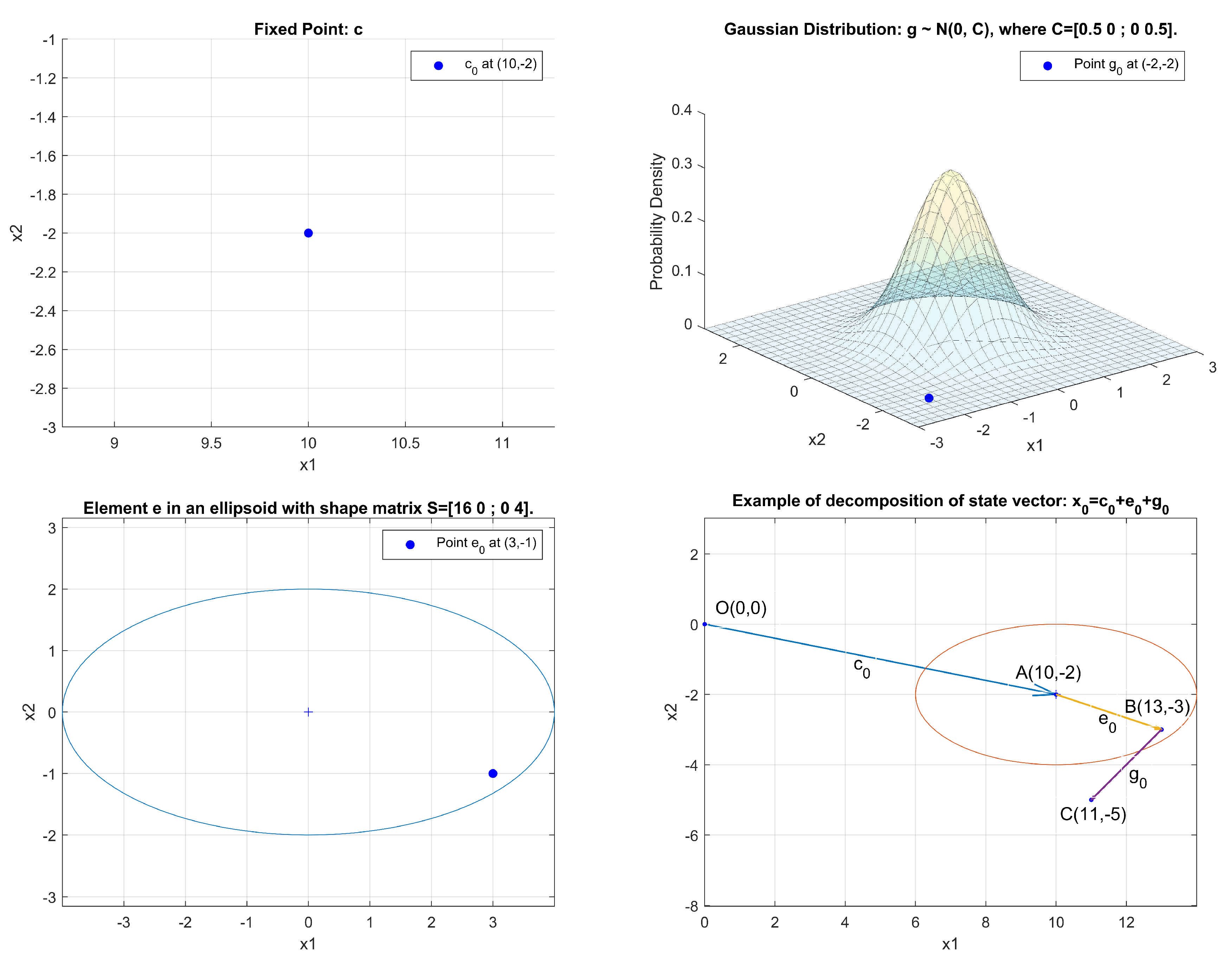
Figure 1 illustrates shows how a state ${\mathbf{x}}_0$ can be decomposed into the sum of the point estimate ${\mathbf{c}}_0$ and two perturbations: the UBB noise component ${\mathbf{e}}_0$ and the Gaussian noise component ${\mathbf{g}}_0$.

Our objective is to use the measurement results to generate the a posteriori estimate ${\widehat{\mathbf{x}}}_0^{+}$, i.e., in precise terms, to compute the point estimate ${\mathbf{c}}_k^{+}$ and the matrices $C_k^{+}$ and $S_k^{+}$.

3. Derivation of Ellipsoidal and Gaussian Kalman Filter

In this section we derive the EGKF model. The derivation is based on the results presented in Section 2.1. The derivation is summarized by the two theorems presented in the following subsection.

3.1. Prediction

As we have mentioned, our algorithm will describe, moment by moment, how our knowledge of the system’s state changes. At the first moment of time, we have information ${\widehat{\mathbf{x}}}_0^{+}$ about the initial state of the system. For each moment $t_k$, $k=0,1,\dots$, our algorithm will describe the transition from moment $t_k$ to the next moment $t_{k+1}$. So, at moment $t_1$, after applying our algorithm, we will know the a posteriori estimate ${\widehat{\mathbf{x}}}_1^{+}$ for the state of the system at this moment. Then, at moment $t_2$, we will get an a posteriori estimate ${\widehat{\mathbf{x}}}_2^{+}$ for the state of the system at moment $t_2$, etc.

Let us describe the transition from moment $t_k$ to the next moment $t_{k+1}$. At moment $t_k$, we know the a posteriori estimate of the state, i.e., we know that

$${\widehat{\mathbf{x}}}_k^{+}={\mathbf{c}}_k^{+}+{\mathbf{g}}_k^{+}+{\mathbf{e}}_k^{+},$$

(17)

where ${\mathbf{g}}_k^{+}\sim \mathrm{N}(\mathbf{0},C_k^{+})$, ${\mathbf{e}}_k^{+}\in \mathcal{E}(\mathbf{0},S_k^{+})$ and ${\mathbf{c}}_k^{+},C_k^{+},S_k^{+}$ are given.

As we showed in the previous section, the a priori estimate at the next moment of time has the form

$${\widehat{\mathbf{x}}}_{k+1}^{-}=F_{x,k}{\widehat{\mathbf{x}}}_k^{+}+{\tilde{\mathbf{u}}}_k+F_{w,k}{\mathbf{w}}_k+F_{a,k}{\mathbf{a}}_k.$$

(18)

The following theorem describes this a prior estimate in the desired form (15).

Theorem 4.

The a priori estimate ${\widehat{\mathbf{x}}}_{k+1}^{-}$, defined by the Formula (18), is equal to: ${\widehat{\mathbf{x}}}_{k+1}^{-}={\mathbf{c}}_{k+1}^{-}+{\mathbf{g}}_{k+1}^{-}+{\mathbf{e}}_{k+1}^{-}$, where

$$\begin{array}{c}{\mathbf{c}}_{k+1}^{-}=F_{x,k}{\mathbf{c}}_k^{+}+{\tilde{\mathbf{u}}}_k,\end{array}$$

(19)

$$\begin{array}{c}{\mathbf{g}}_{k+1}^{-}\sim \mathrm{N}(\mathbf{0},C_{k+1}^{-}),\end{array}$$

(20)

$$\begin{array}{c}{\mathbf{e}}_{k+1}^{-}\in \mathcal{E}(\mathbf{0},S_{k+1}^{-}),\end{array}$$

(21)

$$C_{k+1}^{-}=F_{x,k}{C}_k^{+}{F}_{x,k}^T+F_{w,k}{C}_k^u{F}_{w,k}^T,$$

(22)

and

$$S_{k+1}^{-}=\left(\sqrt{\mathrm{tr}\left(F_{x,k}{S}_k^{+}{F}_{x,k}^T\right)}+\sqrt{\mathrm{tr}\left(F_{a,k}{S}_k^u{F}_{a,k}^T\right)}\right)·\left(\frac{F_{x,k}{S}_k^{+}{F}_{x,k}^T}{\sqrt{\mathrm{tr}\left(F_{x,k}{S}_k^{+}{F}_{x,k}^T\right)}}+\frac{F_{a,k}{S}_k^u{F}_{a,k}^T}{\sqrt{\mathrm{tr}\left(F_{a,k}{S}_k^u{F}_{a,k}^T\right)}}\right).$$

(23)

Proof. 

From (17) and (18), we get

$$\begin{array}{cc}\hfill {\widehat{\mathbf{x}}}_{k+1}^{-}=& F_{x,k}({\mathbf{c}}_k^{+}+{\mathbf{g}}_k^{+}+{\mathbf{e}}_k^{+})+{\tilde{\mathbf{u}}}_k+F_{w,k}{\mathbf{w}}_k+F_{a,k}{\mathbf{a}}_k\hfill \\ \hfill =& F_{x,k}{\mathbf{c}}_k^{+}+F_{x,k}{\mathbf{g}}_k^{+}+F_{x,k}{\mathbf{e}}_k^{+}+{\tilde{\mathbf{u}}}_k+F_{w,k}{\mathbf{w}}_k+F_{a,k}{\mathbf{a}}_k\hfill \\ \hfill =& {\mathbf{c}}_{k+1}^{-}+{\mathbf{g}}_{k+1}^{-}+{\mathbf{e}}_{k+1}^{-},\hfill \end{array}$$

(24)

where we denoted:

$$\begin{array}{c}{\mathbf{c}}_{k+1}^{-}=F_{x,k}{\mathbf{c}}_k^{+}+{\tilde{\mathbf{u}}}_k,\end{array}$$

(25)

$$\begin{array}{c}{\mathbf{g}}_{k+1}^{-}=F_{x,k}{\mathbf{g}}_k^{+}+F_{w,k}{\mathbf{w}}_k,\end{array}$$

(26)

$$\begin{array}{c}{\mathbf{e}}_{k+1}^{-}=F_{x,k}{\mathbf{e}}_k^{+}+F_{a,k}{\mathbf{a}}_k.\end{array}$$

(27)

Here,

$${\mathbf{g}}_k^{+}\sim \mathrm{N}(\mathbf{0},C_k^{+}),{\mathbf{w}}_k\sim \mathrm{N}(\mathbf{0},C_k^u),$$

(28)

therefore according to the properties of Gaussian distributions and (26),

$${\mathbf{g}}_{k+1}^{-}\sim \mathrm{N}(\mathbf{0},C_{k+1}^{-}),$$

(29)

where

$$C_{k+1}^{-}=F_{x,k}{C}_k^{+}{F}_{x,k}^T+F_{w,k}{C}_k^u{F}_{w,k}^T.$$

(30)

Also, here,

$${\mathbf{e}}_k^{+}\in \mathcal{E}(\mathbf{0},S_k^{+}),{\mathbf{a}}_k\in \mathcal{E}(\mathbf{0},S_k^u),$$

(31)

therefore according to Corollary 2:

$${\mathbf{e}}_{k+1}^{-}\in \mathcal{E}(\mathbf{0},S_{k+1}^{-}),$$

(32)

where

$$S_{k+1}^{-}=\left(\sqrt{\mathrm{tr}\left(F_{x,k}{S}_k^{+}{F}_{x,k}^T\right)}+\sqrt{\mathrm{tr}\left(F_a{S}_k^u{F}_a^T\right)}\right)·\left(\frac{F_{x,k}{S}_k^{+}{F}_{x,k}^T}{\sqrt{\mathrm{tr}\left(F_{x,k}{S}_k^{+}{F}_{x,k}^T\right)}}+\frac{F_a{S}_k^u{F}_a^T}{\sqrt{\mathrm{tr}\left(F_a{S}_k^u{F}_a^T\right)}}\right).$$

(33)

The proof is complete. ☐

3.2. Filtering

In the previous section, we show how to generate the a priori estimate for the system’s state. As a result, at each moment $t_k$, we have the following estimate:

$${\widehat{\mathbf{x}}}_k^{-}={\mathbf{c}}_k^{-}+{\mathbf{g}}_k^{-}+{\mathbf{e}}_k^{-},$$

(34)

where ${\mathbf{g}}_k^{-}\sim \mathrm{N}(\mathbf{0},C_k^{-})$, ${\mathbf{e}}_k^{+}\in \mathcal{E}(\mathbf{0},S_k^{-})$ and ${\mathbf{c}}_k^{-},C_k^{-},S_k^{-}$ are known.

Let us now describe how we take the observation results ${\mathbf{y}}_k$ into account, and thus, transform the a priori estimate into an a posteriori one. In line with the general KF idea, to compensate for the prediction error ${\mathbf{y}}_k-h_k({\widehat{\mathbf{x}}}_k^{-},\mathbf{0},\mathbf{0})$, we add, to the a priori estimate, a term proportional to this error, i.e., compute the following a posteriori estimate

$${\widehat{\mathbf{x}}}_k^{+}={\widehat{\mathbf{x}}}_k^{-}+K_k[{\mathbf{y}}_k-h_k({\widehat{\mathbf{x}}}_k^{-},\mathbf{0},\mathbf{0})],$$

(35)

for an appropriate matrix $K_k$. In this section, we consider what happens for a general selection of the gain factor $K_k$. In the next subsection, we will show how to select the optimal gain factor.

Let us show how the resulting a posteriori estimate can be represented in the desired form (15). To come up with this form, we introduce a new parameter $\beta$; the optimal value of this parameter will also be described in the next subsection.

Theorem 5.

Let $\beta >0$. Then, an a posteriori estimate ${\widehat{\mathbf{x}}}_k^{+}$, as defined by the Formula (35), has the form ${\widehat{\mathbf{x}}}_k^{+}={\mathbf{c}}_k^{+}+{\mathbf{g}}_k^{+}+{\mathbf{e}}_k^{+}$, where:

$$\begin{array}{c}{\mathbf{c}}_k^{+}=(I-K_k{H}_{x,k}){\mathbf{c}}_k^{-}+K_k({\mathbf{y}}_k-{\tilde{\mathbf{z}}}_k),\end{array}$$

(36)

$$\begin{array}{c}{\mathbf{g}}_k^{+}\sim \mathrm{N}(\mathbf{0},C_k^{+}),\end{array}$$

(37)

$$\begin{array}{c}{\mathbf{e}}_k^{+}\in \mathcal{E}(\mathbf{0},S_k^{+}),\end{array}$$

(38)

$$C_k^{+}=(I-K_k{H}_{x,k})C_k^{-}{(I-K_k{H}_{x,k})}^T+K_k{H}_{v,k}{C}_k^z{H}_{v,k}^T{K}_k^T,$$

(39)

and

$$S_k^{+}\left(\beta \right)=\left(1+\frac{1}{\beta }\right)(I-K_k{H}_{x,k})S_k^{-}{(I-K_k{H}_{x,k})}^T+(1+\beta )K_k{H}_{b,k}{S}_k^z{H}_{b,k}^T{K}_k^T.$$

(40)

Proof. 

From (34) and (35) we get

$$\begin{array}{cc}\hfill {\widehat{\mathbf{x}}}_k^{+}=& {\widehat{\mathbf{x}}}_k^{-}+K_k[{\mathbf{y}}_k-h_k({\widehat{\mathbf{x}}}_k^{-},\mathbf{0},\mathbf{0})]\hfill \\ \hfill =& {\widehat{\mathbf{x}}}_k^{-}+K_k[{\mathbf{y}}_k-H_{x,k}{\widehat{\mathbf{x}}}_k^{-}-{\tilde{\mathbf{z}}}_k]\hfill \\ \hfill =& (I-K_k{H}_{x,k}){\widehat{\mathbf{x}}}_k^{-}+K_k({\mathbf{y}}_k-{\tilde{\mathbf{z}}}_k)\hfill \\ \hfill =& (I-K_k{H}_{x,k})({\mathbf{c}}_k^{-}+{\mathbf{g}}_k^{-}+{\mathbf{e}}_k^{-})+K_k(H_{x,k}{\mathbf{x}}_k+H_{v,k}{\mathbf{v}}_k+H_{b,k}{\mathbf{b}}_k)\hfill \\ \hfill =& {\mathbf{c}}_k^{+}+{\mathbf{g}}_k^{+}+{\mathbf{e}}_k^k,\hfill \end{array}$$

(41)

where we denoted

$$\begin{array}{c}{\mathbf{c}}_k^{+}=(I-K_k{H}_{x,k}){\mathbf{c}}_k^{-}+K_k{H}_{x,k}{\mathbf{x}}_k,\end{array}$$

(42)

$$\begin{array}{c}{\mathbf{g}}_k^{+}=(I-K_k{H}_{x,k}){\mathbf{g}}_k^{-}+K_k{H}_{v,k}{\mathbf{v}}_k,\end{array}$$

(43)

$$\begin{array}{c}{\mathbf{e}}_k^{+}=(I-K_k{H}_{x,k}){\mathbf{e}}_k^{-}+K_k{H}_{b,k}{\mathbf{b}}_k.\end{array}$$

(44)

For the point estimate part, we have ${\mathbf{v}}_k=\mathbf{0}$ and ${\mathbf{b}}_k=\mathbf{0}$, therefore from (42) we get

$${\mathbf{c}}_k^{+}=(I-K_k{H}_{x,k}){\mathbf{c}}_k^{-}+K_k({\mathbf{y}}_k-{\tilde{\mathbf{z}}}_k).$$

(45)

Here,

$${\mathbf{g}}_k^{-}\sim \mathrm{N}(\mathbf{0},C_k^{-}),{\mathbf{v}}_k\sim \mathrm{N}(\mathbf{0},C_k^z),$$

(46)

therefore according to properties of Gaussian distributions and (37),

$${\mathbf{g}}_k^{+}\sim \mathrm{N}(\mathbf{0},C_k^{+}),$$

(47)

where

$$C_k^{+}=(I-K_k{H}_{x,k})C_k^{-}{(I-K_k{H}_{x,k})}^T+F_{v,k}{C}_k^z{F}_{v,k}^T.$$

(48)

Also here,

$${\mathbf{e}}_k^{-}\in \mathcal{E}(\mathbf{0},S_k^{-}),{\mathbf{b}}_k\in \mathcal{E}(\mathbf{0},S_k^z),$$

(49)

then according to Corollary 1, for any $\beta >0$, we get

$${\mathbf{e}}_k^{+}\in \mathcal{E}(\mathbf{0},S_k^{+}),$$

(50)

where

$$S_k^{+}\left(\beta \right)=\left(1+\frac{1}{\beta }\right)(I-K_k{H}_{x,k})S_k^{-}{(I-K_k{H}_{x,k})}^T+(1+\beta )K_k{H}_{b,k}{S}_k^z{H}_{b,k}^T{K}_k^T.$$

(51)

The proof is complete. ☐

3.3. Optimization Problem

To finalize our algorithm, the only thing left is to find the optimal gain factor $K_k$. Similar to KF and to EKF, we will find the gain factor that minimizes the mean square error of the posteriori estimation.

In our case, this error has two components: the statistical component and the UBB component. To combine these errors into a single objective function, we need to decide how much weight we give to each component. This relative weight will be described by a parameter $\eta \in [0,1]$, so that the resulting cost function will have the following form:

$$J\left(\beta \right)=(1-\eta )\mathrm{tr}\left(C_k^{+}\right)+\eta \mathrm{tr}\left[S_k^{+}\left(\beta \right)\right].$$

(52)

This expression represents the overall uncertainty of the posteriori estimation. We will find the gain factor $K_k$ and the value $\beta$ that minimize this cost function.

Plugging (48) and (51) into (52) we get:

$$\begin{array}{cc}\hfill J\left(\beta \right)=& (1-\eta )\mathrm{tr}\left[(I-K_k{H}_{x,k})C_k^{-}{(I-K_k{H}_{x,k})}^T\right]\hfill \\ \hfill & +(1-\eta )\mathrm{tr}\left[K_k{H}_{v,k}{C}_k^z{H}_{v,k}^T{K}_k^T\right]\hfill \\ \hfill & +\eta \left(1+\frac{1}{\beta }\right)\mathrm{tr}\left[(I-K_k{H}_{x,k})S_k^{-}{(I-K_k{H}_{x,k})}^T\right]\hfill \\ \hfill & +\eta (1+\beta )\mathrm{tr}\left(K_k{H}_{b,k}{S}_k^z{H}_{b,k}^T{K}_k^T\right)\hfill \\ \hfill \triangleq & (1-\eta )\mathrm{tr}\left[(I-K_k{H}_{x,k})C_k^{-}{(I-K_k{H}_{x,k})}^T\right]\hfill \\ \hfill & +(1-\eta )\mathrm{tr}\left[K_k{H}_{v,k}{C}_k^z{H}_{v,k}^T{K}_k^T\right]+\eta \left(1+\frac{1}{\beta }\right)M+\eta (1+\beta )N,\hfill \end{array}$$

(53)

where we denoted $M=\mathrm{tr}\left[(I-K_k{H}_{x,k})S_k^{-}{(I-K_k{H}_{x,k})}^T\right]$ and $N=\mathrm{tr}\left(K_k{H}_{b,k}{S}_k^z{H}_{b,k}^T{K}_k^T\right)$.

Let us first find the optimal value $\beta$. Since $M>0$ and $N>0$, taking into account that the arithmetic mean is always larger than or equal that the geometric mean, we conclude that

$$\left(1+\frac{1}{\beta }\right)M+(1+\beta )N=M+N+\frac{1}{\beta }M+\beta N\ge M+N+2\sqrt{MN}.$$

(54)

In particular, when $\frac{1}{\beta }M=\beta N$, i.e., when $M={\beta }^{2}N$ and $\beta =\sqrt{\frac{M}{N}}$, we have:

$$\left(1+\frac{1}{\beta }\right)M+(1+\beta )N=M+N+2\sqrt{MN}={\left(\sqrt{M}+\sqrt{N}\right)}^2.$$

(55)

Thus, the smallest possible value of the cost function is attained when $\beta =\sqrt{\frac{M}{N}}$. In this case, the cost function $J\left(\beta \right)$, as described by the Formula (52), has the following form:

$$\begin{array}{cc}\hfill J\left(\beta \right)=& (1-\eta )\mathrm{tr}\left[(I-K_k{H}_{x,k})C_k^{-}{(I-K_k{H}_{x,k})}^T\right]\hfill \\ \hfill & +(1-\eta )\mathrm{tr}\left[K_k{H}_{v,k}{C}_k^z{H}_{v,k}^T{K}_k^T\right]+\eta {\left(\sqrt{M}+\sqrt{N}\right)}^2.\hfill \end{array}$$

(56)

To find the optimal value of the gain factor $K_k$, let us differentiate the resulting expression by $K_k$ and equate the resulting derivative to 0.

Notice that

$$\begin{array}{cc}\hfill \frac{\partial \sqrt{M}}{\partial K_k}=& \frac{1}{2}{M}^{-\frac{1}{2}}\frac{\partial M}{\partial K_k}=-\frac{1}{2\sqrt{M}}(I-K_k{H}_{x,k})\left(S_k^{-,T}+S_k^{-}\right)H_{x,k}^T\hfill \\ \hfill =& -\frac{1}{\sqrt{M}}(I-K_k{H}_{x,k})S_k^{-}{H}_{x,k}^T,\hfill \\ \hfill \frac{\partial \sqrt{N}}{\partial K_k}=& \frac{1}{2}{N}^{-\frac{1}{2}}\frac{\partial N}{\partial K_k}=\frac{1}{2\sqrt{N}}{K}_k{H}_{b,k}\left(S_k^{z,T}+S_k^z\right)H_{b,k}^T\hfill \\ \hfill =& \frac{1}{\sqrt{N}}{K}_k{H}_{b,k}{S}_k^z{H}_{b,k}^T.\hfill \end{array}$$

(57)

Therefore,

$$\begin{array}{cc}\hfill \frac{\partial J}{\partial K_k}=& 2(1-\eta )(K_k{H}_{x,k}-I)C_k^{-}{H}_{x,k}^T+2(1-\eta )K_k{H}_{v,k}{C}_k^z{H}_{v,k}^T\hfill \\ \hfill & +2\eta \left(1+\frac{1}{\beta }\right)(K_k{H}_{x,k}-I)S_k^{-}{H}_{x,k}^T+2\eta (1+\beta )K_k{H}_{b,k}{S}_k^z{H}_{b,k}^T.\hfill \end{array}$$

(58)

Equating the resulting derivative $\frac{\partial J}{\partial K_k}$ to 0, we get the following explicit formula for the optimal gain $K_k$:

$$K_k=A^{-1}·\left[(1-\eta )C_k^{-}{H}_{x,k}^T+\eta \left(1+\frac{1}{\beta }\right)S_k^{-}{H}_{x,k}^T\right],$$

(59)

where we denoted:

$$A=(1-\eta )H_{x,k}{C}_k^{-}{H}_{x,k}^T+(1-\eta )H_{v,k}{C}_k^z{H}_{v,k}^T+\eta \left(1+\frac{1}{\beta }\right)H_{x,k}{S}_k^{-}{H}_{x,k}^T+\eta (1+\beta )H_{b,k}{S}_k^z{H}_{b,k}^T.$$

(60)

The only thing left to determine is the parameter $\beta$. For each $\beta$, substituting the expression (48), (51) and (59) into the formula for the cost function, we get the corresponding value of $J\left(\beta \right)$. We thus need to find the value ${\beta }^{*}$ that minimizes this cost function, i.e., that solves the following minimization problem:

$$\begin{array}{cc}\hfill & \underset{\beta }{min}J\left(\beta \right)\hfill \\ \hfill & \mathrm{s}.\mathrm{t}.\beta \in (0,+\infty )\subset {\mathbb{R}}^1.\hfill \end{array}$$

(61)

This optimization problem is more complex than the quadratic optimization problems which usually occur in filtering. Indeed, for quadratic objective functions, derivatives are linear and thus, when we equate all the derivatives to 0, we get an easy-to-solve system of linear equations. In contrast, for non-quadratic objective functions, equating derivatives to 0 leads to a difficult-to-solve system of nonlinear equations. Another reason why non-quadratic optimization problems are often difficult to solve is that traditional methods for solving these problems—such as gradient descent—often lead to a local minimum and not to the desired global minimum of the function. Good news is that in our case, similarly to [27], we can show that the cost function is convex. For convex objective functions, every local minimum is also a global minimum; see, e.g., [28]. Because of this, there exist many efficient techniques for solving convex optimization problems; for example, we can use the corresponding algorithm from the INTLAB toolbox [28].

Once we find the optimal value ${\beta }^{*}$, we can substitute it into the Formulas (48), (51) and (59), and get the desired a posteriori state estimate ${\widehat{\mathbf{x}}}_k^{+}$.

It should be mentioned that this estimate depends on the parameter $\eta$—which was introduced to balance the random uncertainty and UBB uncertainty. Specifically, we should mention three important cases—as described, e.g., in [26]:

(1)

When $\eta =\frac{1}{2}$, the stochastic uncertainty and UBB uncertainty have the same weight. and the optimal gain factor $K_k$ contains no $\eta$ in this case. This setting is recommended to users when there is no expert-based information about $\eta$ available.

(2)

When $\eta =0$, we get:

$$K_k\left(\beta \right)=C_k^{-}{H}_{x,k}^T·{\left[H_{x,k}{C}_k^{-}{H}_{x,k}^T+H_{v,k}{C}_k^z{H}_{v,k}^T\right]}^{-1}.$$

(62)

In this case the filtering model contains no UBB uncertainty and the EGKF algorithm reduces to EKF [6].

(3)

When $\eta =1$, the model now only contains UBB uncertainty. In this case,

$$K_k\left(\beta \right)=\left(1+\frac{1}{\beta }\right)S_k^{-}{H}_{x,k}^T·{\left[\left(1+\frac{1}{\beta }\right)H_{x,k}{S}_k^{-}{H}_{x,k}^T+(1+\beta )H_{b,k}{S}_k^z{H}_{b,k}^T\right]}^{-1}.$$

(63)

Based on Theorems 4 and 5, and Equations (59) and (61), we can summarize the EGKF model into the following Algorithm 1:

Algorithm 1 Ellipsoidal and Gaussian Kalman filter model.
1:	Input: System information: $f_k$, $h_k$, $C_k^u$, $C_k^z$, $S_k^u$, $S_k^z$. Initial values: $c_0^{+}$, $C_0^{+}$, $S_0^{+}$. Parameters: n, $\eta$.
2:	for k=1,2,…,K do
3:	Calculation: $${\mathbf{c}}_k^{-}=F_{x,k-1}{c}_{k-1}^{+}+{\tilde{\mathbf{u}}}_{k-1}.$$ (64) $$C_k^{-}=F_{x,k-1}{C}_{k-1}^{+}{F}_{x,k-1}^T+F_{w,k-1}{C}_{k-1}^u{F}_{w,k-1}^T.$$ (65) $$B=\left(\sqrt{\mathrm{tr}\left(F_{x,k-1}{S}_{k-1}^{+}{F}_{x,k-1}^T\right)}+\sqrt{\mathrm{tr}\left(F_{a,k-1}{S}_{k-1}^u{F}_{a,k-1}^T\right)}\right).$$ (66) $$S_k^{-}=B·\left(\frac{F_{x,k-1}{S}_{k-1}^{+}{F}_{x,k-1}^T}{\sqrt{\mathrm{tr}\left(F_{x,k-1}{S}_{k-1}^{+}{F}_{x,k-1}^T\right)}}+\frac{F_{a,k-1}{S}_{k-1}^u{F}_{a,k-1}^T}{\sqrt{\mathrm{tr}\left(F_{a,k-1}{S}_{k-1}^u{F}_{a,k-1}^T\right)}}\right).$$ (67) $$A=(1-\eta )H_{x,k}{C}_k^{-}{H}_{x,k}^T+(1-\eta )H_{v,k}{C}_k^z{H}_{v,k}^T+\eta \left(1+\frac{1}{\beta }\right)H_{x,k}{S}_k^{-}{H}_{x,k}^T+\eta (1+\beta )H_{b,k}{S}_k^z{H}_{b,k}^T.$$ (68) $$K_k=A^{-1}·\left[(1-\eta )C_k^{-}{H}_{x,k}^T+\eta \left(1+\frac{1}{\beta }\right)S_k^{-}{H}_{x,k}^T\right].$$ (69) $${\mathbf{c}}_k^{+}=(I-K_k{H}_{x,k}){\mathbf{c}}_k^{-}+K_k({\mathbf{y}}_k-{\tilde{\mathbf{z}}}_k).$$ (70) $$C_k^{+}=(I-K_k{H}_{x,k})C_k^{-}{(I-K_k{H}_{x,k})}^T+F_{v,k}{C}_k^z{F}_{v,k}^T.$$ (71) $$\begin{array}{cc}{S}_k^{+}\left(\beta \right)=\hfill & \left(1+\frac{1}{\beta }\right)(I-K_k{H}_{x,k})S_k^{-}{(I-K_k{H}_{x,k})}^T\hfill \\ & +(1+\beta )K_k{H}_{b,k}{S}_k^z{H}_{b,k}^T{K}_k^T.\hfill \end{array}$$ (72) $${\beta }^{*}=arg\underset{\beta >0}{min}\{(1-\eta )\mathrm{tr}\left[C_k^{+}\left(\beta \right)\right]+\eta \mathrm{tr}\left[S_k^{+}\left(\beta \right)\right]\}.$$ (73)
4:	Output:
	${\mathbf{c}}_k^{+}$, $C_k^{+}$, and $S_k^{+}$.
5:	end for

4. Applications

This section contains the result of two test of applying EGKF to simulated data sets. We also applied EKF to both problems, and compared the root-mean-square error (RMSE) of the two methods.

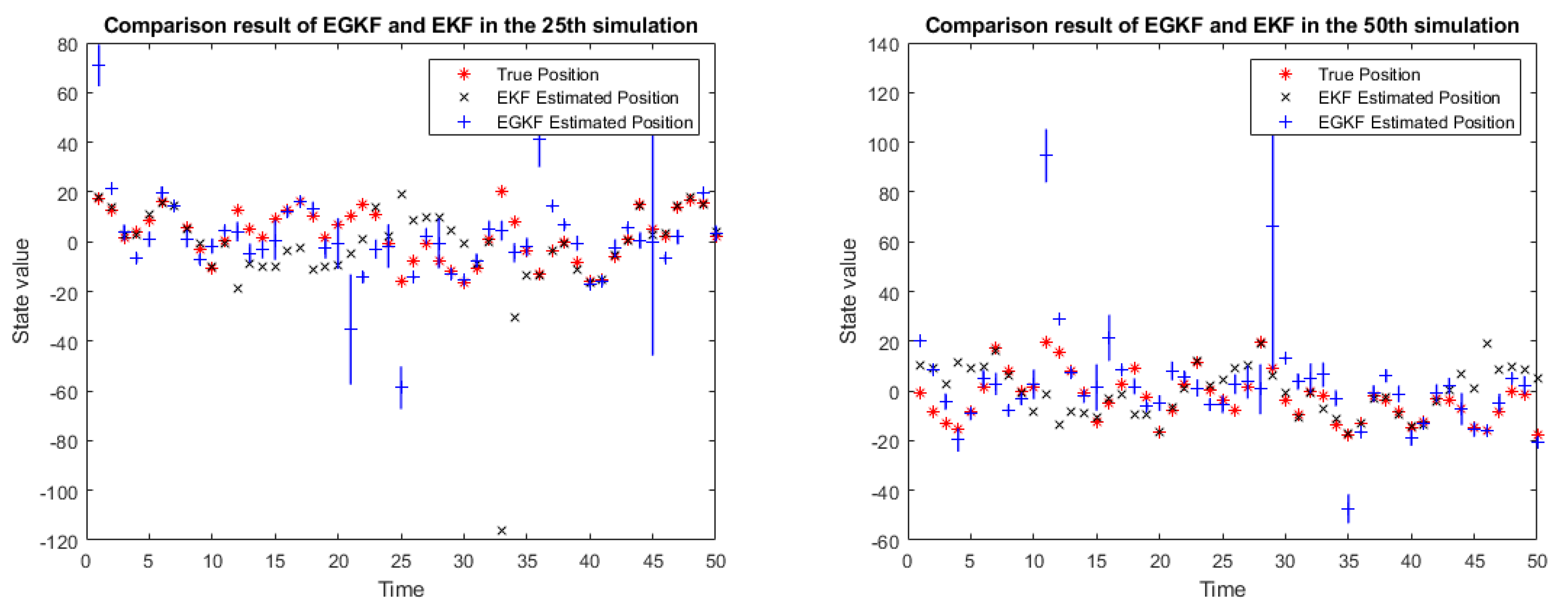
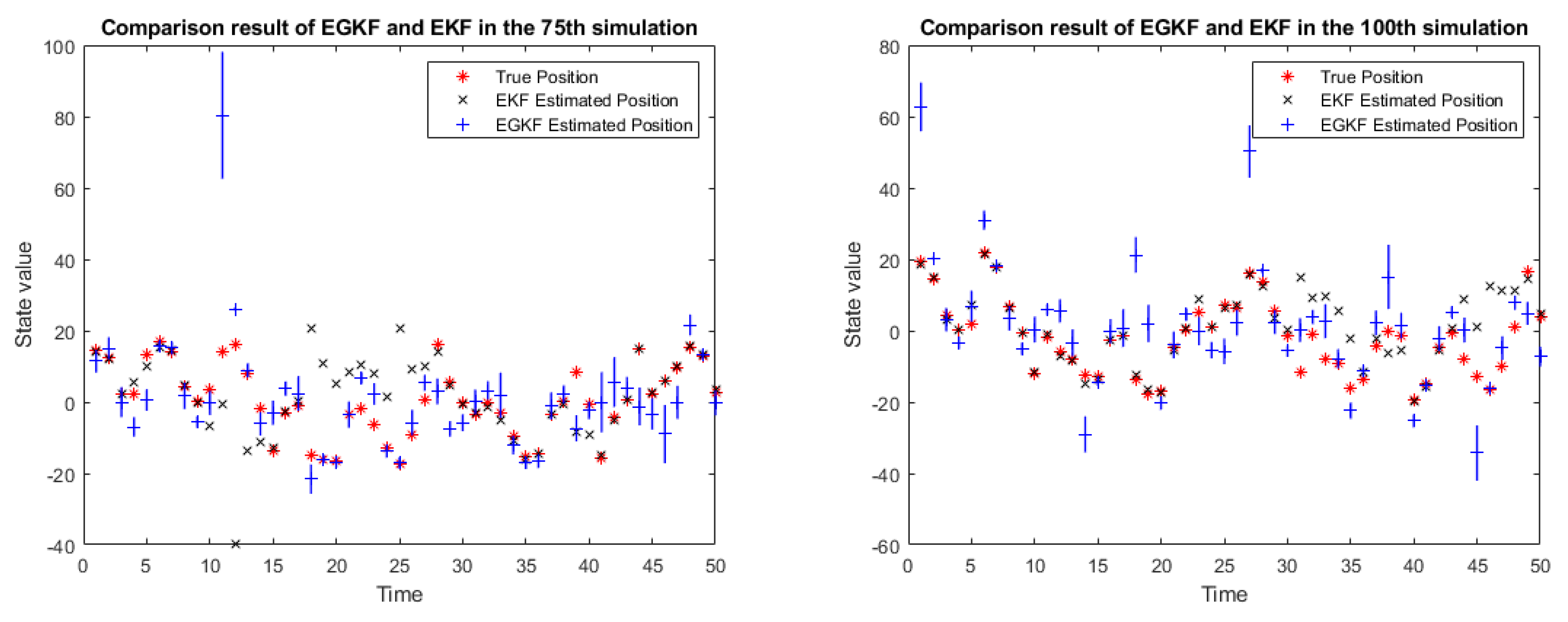
• In the first test, EGKF was applied on a highly nonlinear benchmark problem. To compare the result, we performed 100 simulations.
• In the second test, we applied EGKF on a two-dimensional trajectory estimation problem. For this problem, we performed 1000 Monte Carlo runs.

To simulate the UBB uncertainty, we used uniform distributions on the corresponding ellipsoids.

4.1. Example 1: A Highly Nonlinear Benchmark Example

We consider the following example:

$$\begin{array}{c}{\mathbf{x}}_{k+1}=\frac{1}{2}{\mathbf{x}}_k+\frac{25{\mathbf{x}}_k}{1+{\mathbf{x}}_k^2}+8cos\left[1.2(k-1)\right]+{\mathbf{w}}_k+{\mathbf{a}}_k,\end{array}$$

(74)

$$\begin{array}{c}{\mathbf{y}}_k=\frac{1}{20}{\mathbf{x}}_k^2+{\mathbf{v}}_k+{\mathbf{b}}_k,\end{array}$$

(75)

where:

• ${\mathbf{x}}_k$ is a 1-dimensional scalar,
• ${\mathbf{u}}_k=8cos\left[1.2(k-1)\right]$ is the input vector,
• ${\mathbf{w}}_k\sim \mathrm{N}(\mathbf{0},1)$ is Gaussian noise,
• ${\mathbf{w}}_{i,k}\in \mathcal{E}(\mathbf{0},9)$ is the unknown but bounded perturbation; in this 1-D case the ellipsoid is simply the interval $[-3,3]$,
• ${\mathbf{v}}_k\sim \mathrm{N}(\mathbf{0},1)$ is Gaussian measurement noise,
• ${\mathbf{b}}_k\in \mathcal{E}(\mathbf{0},4)$ is the unknown but bounded perturbation—in this case, the ellipsoid is the interval $[-2,2]$.

Here:

• the initial true state is ${\mathbf{x}}_0=0.1$,
• the initial state estimate is ${\widehat{\mathbf{x}}}_0={\mathbf{x}}_0$,
• the initial estimate for covariance matrix is $C_0^{+}=2$,
• the initial estimate for the shape matrix is $S_0^{+}=1\times {10}^{-3}$.

This discrete-time dynamical system is a known benchmark in the nonlinear estimation theory; see, e.g., [6,8,29]. A high degree of nonlinearity in both process and measurement equations makes state estimation problem for this system very difficult.

We use this example to show that the new EGKF method behaves better than the traditional first order EKF when UBB uncertainties are taken into account.

We used a simulation length of 50 time steps. Following recommendations from the previous section, we selected the weight parameter $\eta =0.5$.

We repeated our simulation 100 times. Figure 2 shows the results of applying both EGKF and EKF for several of the 100 runs, namely, for runs 25, 50, 75, and 100.

In the above figure:

• the red stars denote the true state,
• the black crosses represent the EKF estimates of the state,
• the blue lines represent the UBB ellipsoids estimated by EGKF (in this 1D case they are intervals),
• the blue plus signs mark the centers of the output ellipsoids.

One can see that the centers of the ellipsoids are, in general, different given from the EKF estimates.

For each of the two methods and for each of the 100 iterations, at each moment of time, we can calculate the difference between the actual state and the corresponding estimate. (As estimates corresponding to EGKF, we took the centers of the corresponding a posterior ellipsoids.)

Based on 50 moments of time, we get a vector consisting of 50 such actual-state-vs.-estimated-state differences. To compare the vectors corresponding to two different methods, we calculated the $l_2$ norms of these vectors—this is equivalent to comparing the root-mean-square estimation errors. The resulting values are presented in

Table 1. Comparison of Ellipsoidal and Gaussian Kalman Filter (EGKF) and Extended Kalman Filter (EKF) in 10 simulations.

k	1	11	21	31	41	51	61	71	81	91
EGKF	53.59	116.38	70.38	102.95	100.16	75.81	82.11	48.71	66.30	81.55
EKF	72.49	116.64	230.08	234.69	80.73	31.32	109.53	79.69	8.63	64.95

for simulations 1, 11, …, 91.

In most cases, the EGKF leads to a smaller mean squared estimation error. Over all 100 simulations:

• the average $l_2$ norm of the EGKF estimates is 148.70, while
• for the extended Kalman filter, the average $l_2$ norm is much higher: it is equal to 192.29.

Thus, we conclude that, on average, the new EGKF algorithm performs much better than EKF.

We got a similar conclusion when, instead of comparing the $l_2$ norms, we compared:

• the $l_1$ norms—which correspond to comparing mean absolute values of the estimation errors, and
• the $l_{\infty }$ norms—which correspond to comparing the largest estimation errors.

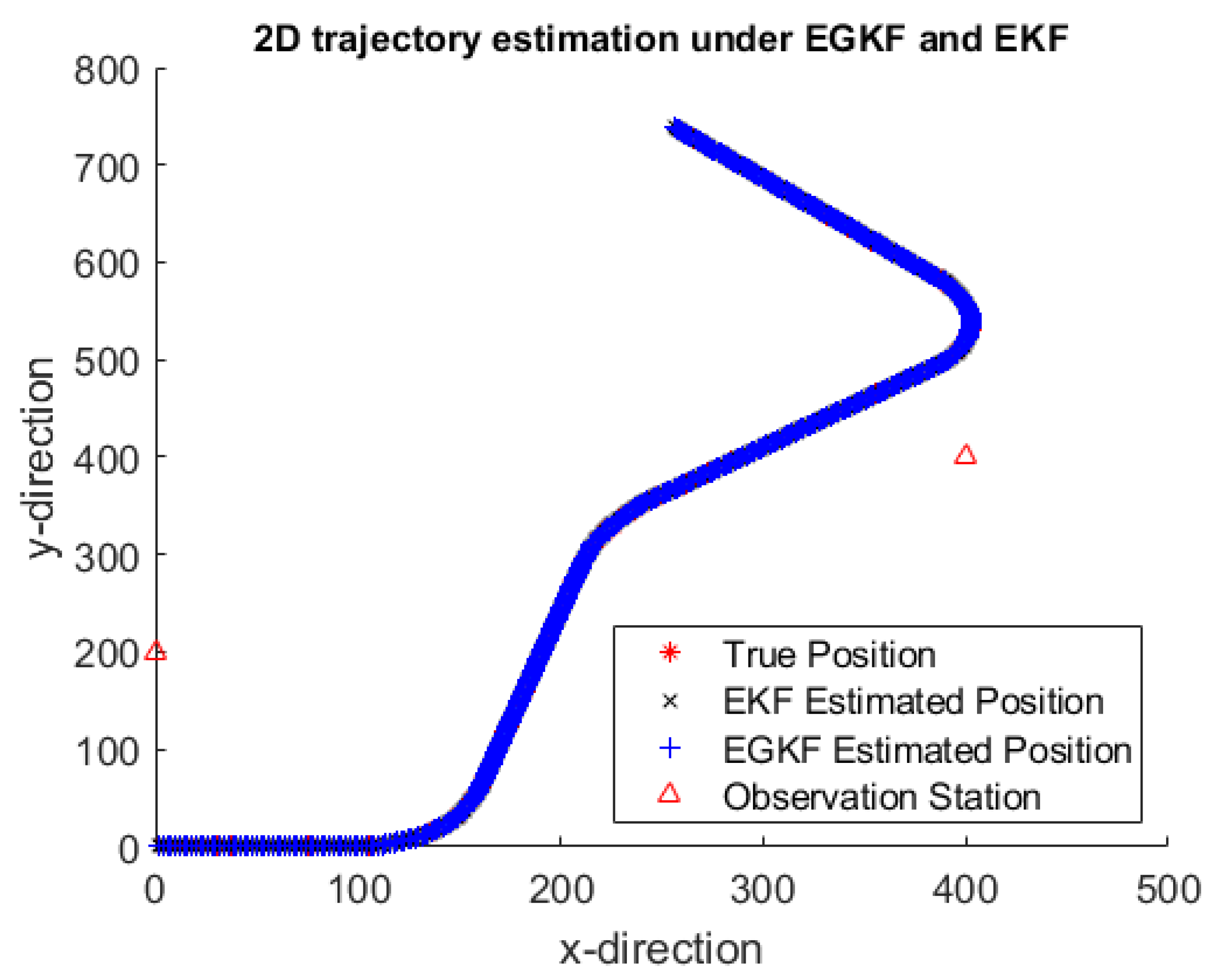
4.2. Example 2: Two-Dimensional Trajectory Estimation

In the second test, we used 1000-times Monte Carlo simulations to compare the performance of EGKF and EKF on a 2D trajectory estimation problem from [10].

In this problem, a vehicle moves on a plane, following a curved trajectory. The state vector $\mathbf{x}=(x,y,v_x,v_y)$ contains positions and velocities of the vehicle, in x-direction and y-direction, respectively. After linearization, we get the following equation:

$${\mathbf{x}}_{k+1}=F_k{\mathbf{x}}_k+{\mathbf{w}}_k+{\mathbf{a}}_k.$$

(76)

Here:

• ${\mathbf{x}}_k=(x_k,y_k,v_{x,k},v_{y,k})$ is the state vector at time $t_k$;
• the transition matrix $F_k$ has the form:

  $$F_k=\left(\begin{array}{cccc}1& 0& \Delta t& 0\\ 0& 1& 0& \Delta t\\ 0& 0& 1& 0\\ 0& 0& 0& 1\end{array}\right);$$

  (77)
• ${\mathbf{w}}_{\mathbf{k}}$ is Gaussian noise with covariance matrix $C_k^u$,
• ${\mathbf{a}}_{\mathbf{k}}$ is the unknown but bounded uncertainty, which is bounded by an ellipsoid with shape matrix $S_k^u$.

In total, in each of the 1000 simulations, we observed 500 epochs with time step $\Delta t=0.1$ s. In our formulas, as units of time, distance, and angle, we chose second, meter and degree, respectively.

In this experiment, two observation stations located at points $S_1=[s_{12},s_{12}]$ and $S_2=[s_{21},s_{22}]$ performed the measurements. Each station measured the distance to the vehicle and the direction to the vehicle, as described by the following equation:

$${\mathbf{y}}_k=\left(\begin{array}{c}{d}_1\\ d_2\\ {\theta }_1\\ {\theta }_2\end{array}\right)=\left(\begin{array}{c}\sqrt{{[x-s_{11}]}^2+{[y-s_{12}]}^2}\\ \sqrt{{[x-s_{21}]}^2+{[y-s_{22}]}^2}\\ arctan[(y-s_{12})/(x-s_{11})]\\ arctan[(y-s_{22})/(x-s_{21})]\end{array}\right)+{\mathbf{v}}_k+{\mathbf{b}}_k.$$

(78)

Here:

• ${\mathbf{v}}_{\mathbf{k}}$ represents random uncertainty; it is Gaussian with covariance matrix $C_k^z$,
• ${\mathbf{b}}_k$ represents the unknown but bounded uncertainty; it is bounded by an ellipsoid with shape matrix $S_k^z$.

The initial state estimate, and initial estimates for the covariance matrix and for the shape matrix are:

• ${\mathbf{x}}_0=(0,0,0,0)$,
• $C_0^{+}=\mathrm{diag}(0.01,0.01,0.01,0.01)$,
• $S_0^{+}=\mathrm{diag}({10}^{-6},{10}^{-6},{10}^{-6},{10}^{-6})$.

The initial covariance matrices in process equation and measurement equation are:

$$C_0^{\mathbf{u}}=\left(\begin{array}{cccc}0.0033& 0& 0.005& 0\\ 0& 0.0033& 0& 0.005\\ 0.005& 0& 0.01& 0\\ 0& 0.005& 0& 0.01\end{array}\right),C_0^z=\left(\begin{array}{cccc}{0.05}^2& 0& 0& 0\\ 0& {0.05}^2& 0& 0\\ 0& 0& {0.01}^2& 0\\ 0& 0& 0& {0.01}^2\end{array}\right).$$

(79)

The initial shape matrices of UBB uncertainties in process equation and measurement equation are:

$$S_0^{\mathbf{u}}=\left(\begin{array}{cccc}{1}^2& 0& 0& 0\\ 0& 1^2& 0& 0\\ 0& 0& {0.5}^2& 0\\ 0& 0& 0& {0.5}^2\end{array}\right),S_0^z=\left(\begin{array}{cccc}{0.01}^2& 0& 0& 0\\ 0& {0.01}^2& 0& 0\\ 0& 0& {\left(\frac{\pi }{180}\right)}^2& 0\\ 0& 0& 0& {\left(\frac{\pi }{180}\right)}^2\end{array}\right).$$

(80)

As in the first example, we select the value $\eta =0.5$ of the weighting parameter.

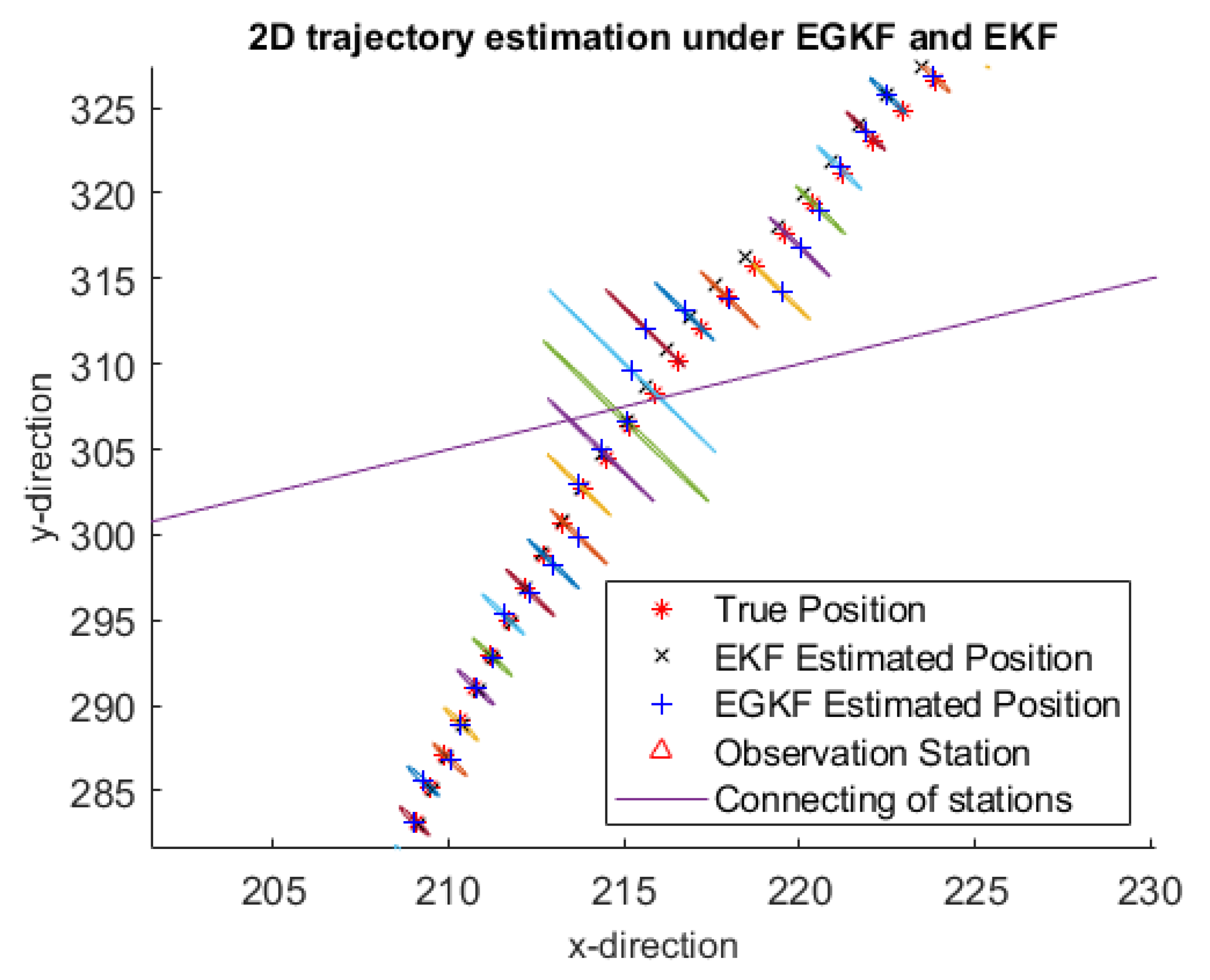
Figure 3 shows an example of trajectory estimates by using EGKF and EKF obtained on one of the 100 iterations—namely, on the 5th iteration. To see it clearer, Figure 4 shows a more detailed information for several portions of the trajectory.

Here:

• the red stars mark the true positions,
• black crosses mark the EKF estimates,
• the blue plus signs are the centers of the ellipsoids computed by EGKF.

The two observation stations are marked by red triangles; they are connected by a straight line.

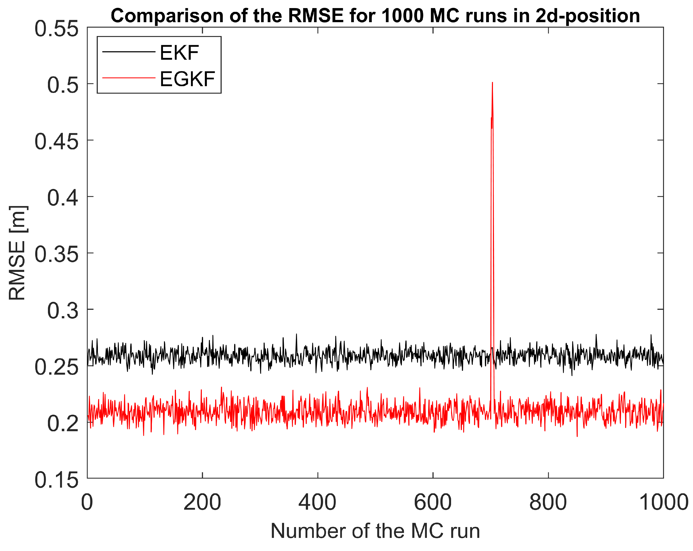
Figure 5 shows the comparison of RMSE estimation errors EGKF and EKF averaged over all 1000 Monte-Carlo runs.

The peak occurred in the figure between [600, 800] is probably caused by the random uncertainty, just like what EKF behaves in nonlinear applications sometimes. In this experiment we introduced new UBB uncertainty but we still kept the influence of random uncertainty ($\eta =0.5$). The new EGKF can provide a better global estimation than EKF but a few exceptions may still happen. This unexpected jump also caused a larger standard deviation value in EGKF.

In almost all simulations (namely, in 997 cases out of 1000), the RMSE of EGKF was significantly smaller than for the EKF. We can therefore conclude that the new EGKF techniques provides better estimation for this nonlinear system than EKF. Detailed statistics of the comparison can be found in

Table 2. RMSE Comparison of EGKF and EKF.

RMSE [m]	EGKF	EKF
Min	0.187	0.241
Max	0.501	0.278
Mean	0.210	0.259
Median	0.209	0.259
Standard Deviation	0.019	0.006

.

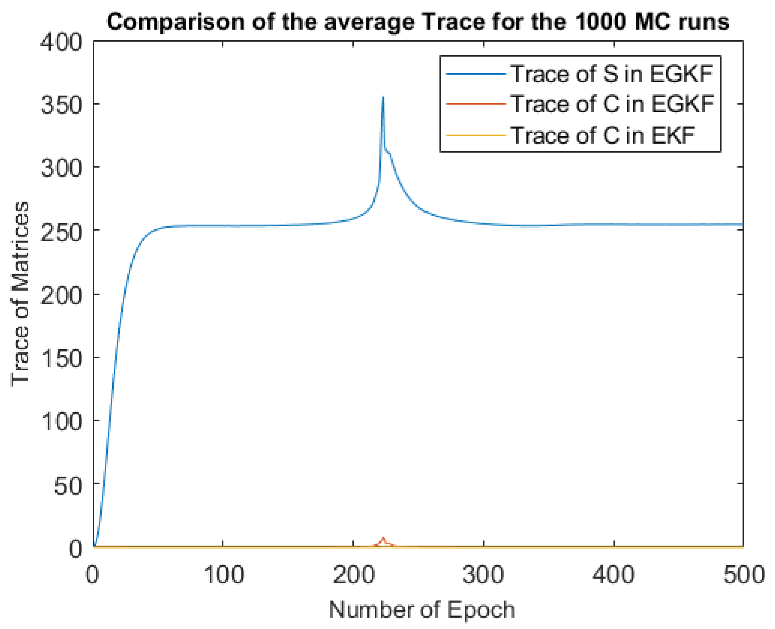
In Figure 6, we compared the average traces (over all 1000 Monte-Carlo runs) of EGKF UBB shape matrix $S_k^{+}$, EGKF covariance matrix $C_k^{+}$ and EKF covariance matrix, in every epoch.

Notice that the trace of EGKF shape matrix is much larger than the traces of covariance matrices.

We can also see that the UBB uncertainty grows in the starting part of the trajectory and when the trajectory crosses the straight line connecting the observation stations—this corresponds to $k\in [210,220]$. This phenomenon is easy to explain: in this case, both angle measurements measure, in effect, the same quantity, so from the measurements, we get fewer information than in other parts of the trajectory.

The EGKF algorithm has been applied to a data set which is obtained from a real world experiment see, e.g., [30]. In that experiment, taken from the scope of georeferencing of terrestrial laser scanner, a multi-sensor system has collected the trajectory information of two GNSS antennas. EGKF was applied to estimate the positions and velocities of those two antennas and the results were compared with EKF.

5. Conclusions and Future Work

In this paper, we propose a new method for state estimation in situations when, in addition to the probabilistic uncertainty, we also have unknown-but-bounded errors. Our testing shows that, on average, the new method leads to much more accurate estimates than the standard extended Kalman filter.

While our method has been shown to be successful, there is room for improvement.

First, the efficiency of our method depends on the initial selection of the parameters describing the system uncertainty and the measurement uncertainties. In some practical situations, we have prior information about these uncertainties, but in other practical cases, we do not have this information. Similarly to the usual Kalman filter, our method eventually converges to the correct uncertainty estimate, but this convergence may be somewhat slow. It would be nice to come up with recommendations on how to select the initial uncertainty parameters that would guarantee faster convergence.

Second, in our method, we assumed that measurements are reasonably frequent, so that during the time interval between the two measurements, we can safely ignore terms quadratic in terms of the corresponding changes—and thus consider a linearized system of equations. This is true in many practical situations—e.g., in the example of GNSS-based navigation that we considered in this paper. However, in some practical situations, measurements are rarer, and so, in the interval between the two measurements, we can no longer ignore terms which are quadratic in terms of changes. To cover such situations, it is desirable to extend our technique to second-order Kalman filtering.

Third, in this paper, we followed the usual Kalman filter techniques in assuming that the corresponding probability distributions are Gaussian. As we mentioned in Section 1, in practice, sometimes distributions are not Gaussian. It is therefore desirable to extend our method to the general non-Gaussian case – e.g., by using ideas of unscented Kalman filtering.

Fourth, in our method, we minimized the mean square estimation error—which, for our method, corresponds to selecting an ellipsoid with the smallest possible trace of the corresponding shape matrix. While in many practical problems, minimizing the mean square error is a reasonable idea, in some problems, it may be more reasonable to minimize, e.g., the largest possible estimation error. In this case, as we have mentioned, instead of minimizing the trace, we should be minimizing the largest eigenvalue of the shape matrix. It is this desirable to extend our method to this—and other—possible criteria.

Fifth, to make computations feasible, we approximated the set of possible states by an ellipsoid. In principle, we can get more accurate estimates if we use families of sets with more parameters for such approximation—e.g., zonotopes or, more generally, generic polytopes. From this viewpoint, it is desirable to come up with efficient algorithms for processing zonotope (and, more generally, polytope) uncertainty.

Finally, it is desirable to analyze (and, if necessary, improve) the stability of our method (and of other state estimation techniques). While stability is very important for practical problems, it is not even clear how to formulate this problem in precise mathematical terms, since the state estimation problems are usually ill-posed—as most inverse problems (see, e.g., [31])—and thus, strictly speaking, not stable.