Analysis and Nonstandard Numerical Design of a Discrete Three-Dimensional Hepatitis B Epidemic Model

Abstract

In this work, we numerically investigate a three-dimensional nonlinear reaction-diffusion susceptible-infected-recovered hepatitis B epidemic model. To that end, the stability and bifurcation analyses of the mathematical model are rigorously discussed using the Routh–Hurwitz condition. Numerically, an efficient structure-preserving nonstandard finite-difference time-splitting method is proposed to approximate the solutions of the hepatitis B model. The dynamical consistency of the splitting method is verified mathematically and graphically. Moreover, we perform a mathematical study of the stability of the proposed scheme. The properties of consistency, stability and convergence of our technique are thoroughly analyzed in this work. Some comparisons are provided against existing standard techniques in order to validate the efficacy of our scheme. Our computational results show a superior performance of the present approach when compared against existing methods available in the literature.

1. Introduction

Hepatitis B is an infectious disease that is a global concern and a major cause of death worldwide [1]. This disease is disseminated by means of the hepatitis B virus (HBV) through various forms of transmission. Indeed, a susceptible person may be infected through blood transfusion, exchange of saliva, use of contaminated razors and needles, sexual contact with an infected person, and even through acupuncture and piercing instruments, among other forms of transmission [2]. Moreover, it is well known that infected pregnant women may also transmit the HBV to the fetus [3]. To this day, many studies have been conducted in order to understand the mechanisms of transmission of hepatitis B. As a consequence of those studies, nowadays we count with prevention measures, diagnosis tests, protocols to treat the chronic hepatitis B [4], and even some regional studies have proposed more efficient management measures to treat hepatitis B based on geographical and social factors [5,6]. At the same time, there are rigorous reports which investigate the epidemiological problem from a world-wide perspective [7].

It is important to recall that hepatitis B has two phases. The first phase of the disease is called acute hepatitis B infection [8], and it spans for approximately the first six months after a person is infected. In general, infected individuals reflect no symptoms during this phase, and the symptoms can not be easily diagnosed. Most of the infected individuals (about 90 percent) have a strong immune system which fights off the infection during the first six months of the acute phase [9]. Except in some cases in which individuals have some immunological deficiency, the HBV is completely controlled and the liver heals until it becomes healthy [10]. It is well know that those subjects become immune to HBV for the rest of their life. Unfortunately, those individuals who do not have a sufficiently strong immune system cannot heal completely during the rest of their lives. In fact, this persistent state of HBV is the second phase of hepatitis B, and it is called the chronic phase [11]. At the chronic stage the liver is swollen and presents cirrhosis. Ultimately, HBV is a serious potential cause of hepatocellular carcinoma and other types of cancer [12].

Mathematically, there are various reports on the modeling of the propagation of diseases [13,14,15,16]. In addition to reports on the modeling of the transmission of hepatitis B [10,17], there are also studies on the co-dynamics of pneumonia and typhoid fever diseases with cost effective optimal control analysis [18], the mathematical modeling of hepatitis C treatment for injecting drug users [19] and the epidemiological modeling of the propagation of cholera with optimal control treatment [20]. Other mathematical models have been proposed also to model and control the dynamics of propagation of vector-borne diseases such as malaria [21], zika [22] and dengue [23], and there are even some recent reports which investigate thoroughly the influence of climate, environmental and socio-economic change on the dynamics of transmission of vector-borne diseases [24]. In those reports, the models employed to describe the dynamics of propagation of illnesses consist of systems of ordinary or partial differential equations [25] and, in all of them, the incidence of the disease plays a decisive role in its dynamics. In fact, the transmission of these illnesses can be studied comprehensively by introducing suitable incidence rate in the quantitative models.

In this manuscript, we will employ saturated incidence rates on both the susceptible and the infected populations. It is worth noting that this approach has been successfully used by some authors in the recent literature [26,27,28]. More concretely, the present work is motivated by the following susceptible-infected-recovered model for hepatitis B with saturated incidence rates:

$$\left\{\begin{array}{cc}\frac{d{X}_1\left(t\right)}{dt}\hfill & =\lambda -\frac{\alpha X_1\left(t\right)X_2\left(t\right)}{1+\gamma X_2\left(t\right)}-({\mu }_0+\nu )X_1\left(t\right),\forall t>0,\hfill \\ \frac{d{X}_2\left(t\right)}{dt}\hfill & =\frac{\alpha X_1\left(t\right)X_2\left(t\right)}{1+\gamma X_2\left(t\right)}-({\mu }_0+{\mu }_1+\beta )X_2\left(t\right),\forall t>0,\hfill \\ \frac{d{X}_3\left(t\right)}{dt}\hfill & =\beta X_2\left(t\right)+\nu X_1\left(t\right)-{\mu }_0{X}_3\left(t\right),\forall t>0.\hfill \end{array}\right.$$

(1)

In this model, $X_1,X_2,X_3:{\mathbb{R}}^{+}\cup \left\{0\right\}\to \mathbb{R}$ are sufficiently smooth functions that represent the total of susceptible, infected and recovered individuals, respectively. This model was proposed recently in [29] as a mathematical model of transmission of hepatitis B, and its inhibition effects are the most notable physical features. Here, $\alpha$ and $\lambda$ represent, respectively, the transmission and birth rates. Meanwhile, ${\mu }_0$ and ${\mu }_1$ are the natural and disease-induced death rates, respectively. The recovery rate is given by $\beta$, while the vaccination and saturation rates are $\nu$ and $\gamma$, respectively.

The present model has the novelty that it considers saturated incidence rates, and it has various biological and mathematical properties. In particular, it is worth pointing out that this model has a positive invariance, positive solutions exist and considers different epidemiological states. More precisely, disease free and endemic states exist for this model. The system (1) has a basic reproductive number, which is calculated using a matrix approach. Linear stability theory can be easily applied to discuss the local dynamics and obtain the stability conditions in terms of the basic reproductive number. Central manifold theory shows that the proposed model exhibits the backward bifurcation phenomenon. In turn, the global stability of the model can be discussed using Lypanov function theory. Moreover, the local sensitivity analysis was discussed in [29] along with the development of an optimal control mechanism. Furthermore, this model has been validated for large-scale scenarios, and the feasibility of its optimization has been thoroughly established.

Observe that we may assume that the system (1) takes on the reduced form

$$\left\{\begin{array}{cc}\hfill \frac{d{X}_1\left(t\right)}{dt}& =\lambda -\frac{\alpha X_1\left(t\right)X_2\left(t\right)}{1+\gamma X_2\left(t\right)}-({\mu }_0+\nu )X_1\left(t\right),\forall t>0,\hfill \\ \hfill \frac{d{X}_2\left(t\right)}{dt}& =\frac{\alpha X_1\left(t\right)X_2\left(t\right)}{1+\gamma X_2\left(t\right)}-({\mu }_0+{\mu }_1+\beta )X_2\left(t\right),\forall t>0.\hfill \end{array}\right.$$

(2)

Notice that this step is justified by the fact that the dynamics of $X_1$ and $X_2$ does not depend on $X_3$, indeed. Obviously, the system (2) represents the dynamics of a homogeneous population. A more realistic approach would be to consider non-homogeneous populations in view that the disease may spread at different rates in different directions. To that end, for the remainder of this work, we let $p\in \{1,2,3\}$ and suppose that $B\subseteq {\mathbb{R}}^p$ is a spatial domain. Throughout, let $T\in {\mathbb{R}}^{+}$ be a temporal period, and define $\Omega =B\times (0,T)$. Let $X_1,X_2,X_3:\overline{\Omega }\to \mathbb{R}$ and ${\rho }_1,{\rho }_2:B\to \mathbb{R}$ be functions.

For the sake of concreteness, $X_1(\mathbf{x},t)$ denotes the density of individuals that are susceptible to HBV at the point $(\mathbf{x},t)\in \overline{\Omega }$. Meanwhile, $X_2(\mathbf{x},t)$ and $X_3(\mathbf{x},t)$ denote the respective densities of infected and recovered individuals, respectively. In this work, we will study the system

$$\left\{\begin{array}{cc}\hfill \frac{\partial X_1(\mathbf{x},t)}{\partial t}& =d_1\Delta X_1(\mathbf{x},t)+\lambda -\frac{\alpha X_1(\mathbf{x},t)X_2(\mathbf{x},t)}{1+\gamma X_2(\mathbf{x},t)}-({\mu }_0+\nu )X_1(\mathbf{x},t),\forall (\mathbf{x},t)\in \Omega ,\hfill \\ \hfill \frac{\partial X_2(\mathbf{x},t)}{\partial t}& =d_2\Delta X_2(\mathbf{x},t)+\frac{\alpha X_1(\mathbf{x},t)X_2(\mathbf{x},t)}{1+\gamma X_2(\mathbf{x},t)}-({\mu }_0+{\mu }_1+\beta )X_2(\mathbf{x},t),\forall (\mathbf{x},t)\in \Omega .\hfill \end{array}\right.$$

(3)

Here, $\Delta$ represents the usual Laplacian in the spatial coordinates and, in the particular case of the spatially three-dimensional scenario, $\mathbf{x}=(x,y,z)\in \overline{\Omega }$. Moreover, we will consider homogeneous Neumann boundary data along with the initial conditions

$$\begin{array}{cc}\hfill X_1(x,0)& ={\rho }_1\left(x\right)\ge 0,\forall x\in B,\hfill \end{array}$$

(4)

$$\begin{array}{cc}\hfill X_2(x,0)& ={\rho }_2\left(x\right)\ge 0,\forall x\in B.\hfill \end{array}$$

(5)

We must point out that the variables of interest of (3) are actually population densities. In general, the positivity of solutions is an important feature in the investigation of systems where the unknown quantities are measured in absolute scales [30,31]. In the recent years, various numerical schemes which preserve the positivity have been proposed for the numerical study of various physical problems. As examples, some positivity-preserving finite-difference methods have been proposed to study some weakly coupled systems of partial differential equations describing the dynamics of interaction between a colony of bacteria and a substrate of nutrients [32], reaction-diffusion equations [33], the three-dimensional Brusselator reaction diffusion system [34], Fisher’s equation [35], physical model with transport memory and nonlinear damping [36], damped nonlinear wave equations [37] and generalized Burgers–Huxley-type systems [30]. The present manuscript is devoted to designing and analyzing a positivity-preserving finite-difference scheme to solve numerically the system (3).

This work is sectioned as follows. The steady states and reproductive value of the model under investigation are discussed in Section 2. In the same section, we also perform a linear stability analysis of the model (3), and investigate the bifurcation value of the parameter $\alpha$. Section 3 is devoted to introducing the numerical schemes to solve the diffusive hepatitis B model. We will provide the necessary discrete nomenclature, and we will introduce therein a backward Euler splitting technique and a nonstandard finite-difference operator splitting method [38,39]. It is worth pointing out that the design of the nonstandard technique will observe literally the set of rules proposed by R. E. Mickens [40]. The theoretical analysis of the schemes will be performed in Section 4. We will show that the nonstandard scheme is capable of preserving the positivity of the approximations, and that it is an accurate, stable and convergent technique. Some computational results are shown in Section 5. The simulations will shed light on the validity of the theoretical results obtained in this work.

2. Qualitative Analysis

This section is devoted to establishing qualitative properties of the system (3). Firstly, notice that there are two equilibrium points of the system. Those points will be referred to as the disease-free equilibrium point (DFEP) and the endemic equilibrium point (EEP), and they are given respectively by

$${\epsilon }_0=\left(\frac{\lambda }{({\mu }_0+\nu )},0\right)\mathrm{and}{\epsilon }_{\ast }=({X_1}_{\ast },{X_2}_{\ast }),$$

(6)

where

$$\begin{array}{cc}\hfill {X_1}_{\ast }& =\frac{1}{\alpha }({\mu }_0+{\mu }_1+\beta )(1+\gamma {X_2}_{\ast }),\hfill \end{array}$$

(7)

$$\begin{array}{cc}\hfill {X_2}_{\ast }& =\frac{({\mu }_0+\nu )}{(\alpha +\gamma ({\mu }_0+\nu ))}(B_0-1).\hfill \end{array}$$

(8)

Note that the reproductive number of the system (3) when $d_1=d_2=0$ is given by

$$B_0=\frac{\alpha \lambda }{({\mu }_0+\nu )({\mu }_0+{\mu }_1+\beta )}.$$

(9)

2.1. Stability

In order to carry out the stability analysis of the system (3), we linearize it around the point $({X_1}_{\ast },{X_2}_{\ast })$ considering small perturbations on $X_1(\mathbf{x},t)$ and $X_2(\mathbf{x},t)$. More precisely, we consider

$$\left\{\begin{array}{cc}\hfill \frac{\partial X_1(\mathbf{x},t)}{\partial t}& =v_{11}{X}_1(\mathbf{x},t)+v_{12}{X}_2(\mathbf{x},t)+d_1\Delta X_1(\mathbf{x},t),\forall (\mathbf{x},t)\in \Omega ,\hfill \\ \hfill \frac{\partial X_2(\mathbf{x},t)}{\partial t}& =v_{21}{X}_1(\mathbf{x},t)+v_{22}{X}_2(\mathbf{x},t)+d_2\Delta X_2(\mathbf{x},t),\forall (\mathbf{x},t)\in \Omega .\hfill \end{array}\right.$$

(10)

Departing now from the system of Equation (10), we calculate the Fourier series solution. As a consequence, the variational matrix $\mathfrak{V}$ for that system is given by

$$\mathfrak{V}=\left(\begin{array}{cc}{v}_{11}-d_1{\kappa }_1^2-d_1{\kappa }_2^2-d_1{\kappa }_3^2-\Lambda & v_{12}\\ v_{21}& v_{22}-d_2{\kappa }_1^2-d_2{\kappa }_2^2-d_2{\kappa }_3^2-\Lambda \end{array}\right).$$

(11)

Here, ${\kappa }_i$ represents the wave number for the node $n_i$, for each $i=1,2,3$. Concretely, for $n_1,n_2,n_3\in \mathbb{Z}$,

$${\kappa }_1=n_1\pi /2,{\kappa }_2=n_2\pi /2,{\kappa }_3=n_3\pi /2.$$

(12)

Additionally, we define the set of constants

$$\left\{\begin{array}{cc}\hfill v_{11}& =-\frac{\alpha {X_2}_{\ast }}{1+\gamma {X_2}_{\ast }}-({\mu }_0+\nu ),\hfill \\ \hfill v_{12}& =-\frac{\alpha {X_1}_{\ast }}{{(1+\gamma {X_2}_{\ast })}^2},\hfill \\ \hfill v_{21}& =\frac{\alpha {X_2}_{\ast }}{1+\gamma {X_2}_{\ast }},\hfill \\ \hfill v_{22}& =\frac{\alpha {X_1}_{\ast }}{{(1+\gamma {X_2}_{\ast })}^2}-({\mu }_0+{\mu }_1+\beta ).\hfill \end{array}\right.$$

(13)

Note that the characteristic equation of $\mathfrak{V}$ is ${\Lambda }^2+{\vartheta }_1\Lambda +{\vartheta }_2=0$, where

$${\vartheta }_1=d_1{\kappa }_1^2+d_1{\kappa }_2^2+d_2{\kappa }_1^2+d_1{\kappa }_3^2+d_2{\kappa }_2^2+d_2{\kappa }_3^2-v_{22}-v_{11}$$

(14)

and

$$\begin{array}{cc}\hfill {\vartheta }_2& =v_{11}{v}_{22}-v_{12}{v}_{21}-v_{11}{d}_2{\kappa }_1^2-v_{11}{d}_2{\kappa }_2^2-v_{11}{d}_2{\kappa }_3^2-v_{22}{d}_1{\kappa }_1^2-v_{22}{d}_1{\kappa }_2^2\hfill \\ \hfill & -v_{22}{d}_1{\kappa }_3^2+d_1{d}_2{\kappa }_1^4+d_1{d}_2{\kappa }_2^4+d_1{d}_2{\kappa }_3^4+2d_1{d}_2{\kappa }_1^2{\kappa }_2^2+2d_1{d}_2{\kappa }_1^2{\kappa }_3^2+2d_1{d}_2{\kappa }_2^2{\kappa }_3^2.\hfill \end{array}$$

(15)

In turn, the stability criterion discussed by the Routh–Hurwitz requires that ${\vartheta }_1>0$ and ${\vartheta }_2>0$.

2.2. Bifurcation Value

We discuss now the bifurcation value of $\alpha$. To this end, we used the values of model parameters presented in

Table 1. Values of the model parameters used in [29].

$\mathit{\lambda }$	$\mathit{\gamma }$	$\mathit{\nu }$	$\mathit{\beta }$	$\mathit{\alpha }$	${\mathit{\mu }}_0$	${\mathit{\mu }}_1$
$0.232$	$0.9$	$0.2$	$4.12$	$7.9$	$0.000232$	$0.0000547$

. Substituting all the values of parameters other than $\alpha$ into (13), we obtain

$$\begin{array}{ccc}\hfill v_{11}& =-\frac{\left(b_1(b_2{\alpha }^2+b_3\alpha +b_4)\right)}{\left(b_5(b_6\alpha +b_7)\right)},\hfill & \hfill v_{12}=-\frac{(b_8\alpha +b_9)}{\left(b_{10}(b_{11}\alpha +b_{12})\right)},\end{array}$$

(16)

$$\begin{array}{ccc}\hfill v_{21}& =\frac{\left(b_{13}\alpha (b_{14}\alpha -b_{15})\right)}{(b_{16}\alpha +b_{17})},\hfill & \hfill v_{22}=-\frac{\left(b_{18}(b_{19}\alpha -b_{20})\right)}{\left(b_{21}(b_{22}\alpha +b_{23})\right)},\end{array}$$

(17)

where,

$$\left\{\begin{array}{ccc}\hfill b_1& =3.60705904\times {10}^{15},\hfill & \hfill b_2=2.35275951\times {10}^{34},\\ \hfill b_3& =4.23987968\times {10}^{33},\hfill & \hfill b_4=b_{15}=b_{17}=b_{20}=9.28882337\times {10}^{17},\\ \hfill b_5& =5.40431955\times {10}^{16},\hfill & \hfill b_6=b_{11}=b_{22}=2.93020542\times {10}^{34},\\ \hfill b_7=b_{12}& =3.09627445\times {10}^{17},\hfill & \hfill b_8=2.58753620\times {10}^{50},\\ \hfill b_9& =4.66296794\times {10}^{49},\hfill & \hfill b_{10}=b_{21}=2.25179981\times {10}^{15},\\ \hfill b_{13}& =1.80352952\times {10}^{16},\hfill & \hfill b_{14}=b_{19}=2.61208778\times {10}^{17},\\ \hfill b_{16}& =8.79061626\times {10}^{34},\hfill \\ \hfill b_{18}& =5.01997697\times {10}^{31},\hfill & \hfill b_{23}=3.09627445\times {10}^{17}.\end{array}\right.$$

(18)

On the other hand,

$$\begin{array}{c}\hfill {\vartheta }_1=\frac{(a_1{\alpha }^2+a_2\alpha -a_3)}{\left(a_4(a_5\alpha +a_6)\right)}={\mathcal{F}}_1\left(\alpha \right),\end{array}$$

(19)

where

$$\left\{\begin{array}{ccc}\hfill a_1& =1.08627743\times {10}^{52},\hfill & \hfill a_2=5.87440522\times {10}^{52},\\ \hfill a_3& =1.43246375\times {10}^{53},\hfill & \hfill a_4=6.91752902\times {10}^{18},\\ \hfill a_5& =2.93020542\times {10}^{34},\hfill & \hfill a_6=3.09627445\times {10}^{17}.\end{array}\right.$$

(20)

Finally,

$$\begin{array}{c}\hfill {\vartheta }_2=-\frac{(-c_1{\alpha }^2+c_2\alpha +c_3)}{\left(c_4(c_5\alpha +c_6)\right)}={\mathcal{F}}_2\left(\alpha \right),\end{array}$$

(21)

where

$$\left\{\begin{array}{ccc}\hfill c_1& =4.00766089\times {10}^{67},\hfill & \hfill c_2=1.32418810\times {10}^{68},\\ \hfill c_3& =2.61620849\times {10}^{67},\hfill & \hfill c_4=6.08472288\times {10}^{33},\\ \hfill c_5& =2.93020542\times {10}^{34},\hfill & \hfill c_6=3.09627445\times {10}^{17}.\end{array}\right.$$

(22)

Notice that ${\mathcal{F}}_2\left(\alpha \right)=0$ gives the bifurcation value of $\alpha$, which changes from stable to unstable the nature of the EEP. This value is given by $\alpha =3.4911307434$. Thus, EEP is stable for any value of $\alpha$ greater than or equal to $3.4911307434$, and unstable for any value which is less than $3.4911307434$.

3. Numerical Models

For the remainder of this work, we assume that $B={(0,L)}^3\subseteq {\mathbb{R}}^3$, with $L\in {\mathbb{R}}^{+}$. Let ${\mathcal{M}}_1,{\mathcal{M}}_2\in \mathbb{N}$, and divide $\overline{\Omega }$ into ${\mathcal{M}}_1^3\times {\mathcal{M}}_2$ hypercubes, using a spatial step-size of length $\Delta x=(b-a)/{\mathcal{M}}_1$ on each of the three spatial edges, and a temporal step-size equal to $\Delta t=T/{\mathcal{M}}_2$. More precisely, the grid points are of the form $(x_{m_1},y_{m_2},z_{m_3})\in {\mathbb{R}}^3$, with

$$x_{m_1}=m_1\Delta x,y_{m_2}=m_2\Delta x,z_{m_3}=m_3\Delta x,$$

(23)

for each $m_1,m_2,m_3=0,1,\dots ,{\mathcal{M}}_1$. Meanwhile, we let $t_k=k\Delta t$, for each $k=0,1,\dots ,{\mathcal{M}}_2$. Finally, we use the symbol ${X_1}_{m_1,m_2,m_3}^k$ to represent any finite-difference approximations to the exact value of $X_1(m_1\Delta x,m_2\Delta x,m_3\Delta x,k\Delta t)$, and ${X_2}_{m_1,m_2,m_3}^k$ is the respective estimate of $X_2(m_1\Delta x,m_2\Delta x,m_3\Delta x,k\Delta t)$.

3.1. Backward Euler Scheme

The Backward Euler splitting method will hinge on approximating the solution of a time-split form of (3). More precisely, we will consider the following two four-step sets:

$$\left\{\begin{array}{cc}\hfill \frac{1}{4}\frac{\partial X_1(\mathbf{x},t)}{\partial t}& =\lambda -\frac{\alpha X_1(\mathbf{x},t)X_2(\mathbf{x},t)}{1+\gamma X_2(\mathbf{x},t)}-({\mu }_0+\nu )X_1(\mathbf{x},t),\forall (\mathbf{x},t)\in \Omega ,\hfill \\ \hfill \frac{1}{4}\frac{\partial X_1(\mathbf{x},t)}{\partial t}& =d_1\frac{{\partial }^2{X}_1(\mathbf{x},t)}{\partial x^2},\forall (\mathbf{x},t)\in \Omega ,\hfill \\ \hfill \frac{1}{4}\frac{\partial X_1(\mathbf{x},t)}{\partial t}& =d_1\frac{{\partial }^2{X}_1(\mathbf{x},t)}{\partial y^2},\forall (\mathbf{x},t)\in \Omega ,\hfill \\ \hfill \frac{1}{4}\frac{\partial X_1(\mathbf{x},t)}{\partial t}& =d_1\frac{{\partial }^2{X}_1(\mathbf{x},t)}{\partial z^2},\forall (\mathbf{x},t)\in \Omega .\hfill \end{array}\right.$$

(24)

and

$$\left\{\begin{array}{cc}\hfill \frac{1}{4}\frac{\partial X_2(\mathbf{x},t)}{\partial t}& =\frac{\alpha X_1(\mathbf{x},t)X_2(\mathbf{x},t)}{1+\gamma X_2(\mathbf{x},t)}-({\mu }_0+{\mu }_1+\beta )X_2(\mathbf{x},t),\forall (\mathbf{x},t)\in \Omega ,\hfill \\ \hfill \frac{1}{4}\frac{\partial X_2(\mathbf{x},t)}{\partial t}& =d_2\frac{{\partial }^2{X}_2(\mathbf{x},t)}{\partial x^2},\forall (\mathbf{x},t)\in \Omega ,\hfill \\ \hfill \frac{1}{4}\frac{\partial X_2(\mathbf{x},t)}{\partial t}& =d_2\frac{{\partial }^2{X}_2(\mathbf{x},t)}{\partial y^2},\forall (\mathbf{x},t)\in \Omega ,\hfill \\ \hfill \frac{1}{4}\frac{\partial X_2(\mathbf{x},t)}{\partial t}& =d_2\frac{{\partial }^2{X}_2(\mathbf{x},t)}{\partial z^2},\forall (\mathbf{x},t)\in \Omega .\hfill \end{array}\right.$$

(25)

Let $k=0,1,\dots ,{\mathcal{M}}_2-1$. At the kth temporal step, the Backward Euler splitting approximation of the susceptible component $X_1$ at the first splitting step is given as

$$\begin{array}{c}\hfill \frac{{X_1}_{m_1,m_2,m_3}^{k+\frac{1}{4}}-{X_1}_{m_1,m_2,m_3}^k}{\Delta t}=\lambda -\frac{\alpha {X_1}_{m_1,m_2,m_3}^k{X_2}_{m_1,m_2,m_3}^k}{1+\gamma {X_2}_{m_1,m_2,m_3}^k}-({\mu }_0+\nu ){X_1}_{m_1,m_2,m_3}^k\end{array}$$

(26)

After simplification, we readily reach that

$${X_1}_{m_1,m_2,m_3}^{k+\frac{1}{4}}={X_1}_{m_1,m_2,m_3}^k+\Delta t\lambda -\Delta t\frac{\alpha {X_1}_{m_1,m_2,m_3}^k{X_2}_{m_1,m_2,m_3}^k}{1+\gamma {X_2}_{m_1,m_2,m_3}^k}-\Delta t({\mu }_0+\nu ){X_1}_{m_1,m_2,m_3}^k.$$

(27)

In similar fashion, the formulas for the second, third and fourth steps are, respectively,

$$\begin{array}{cc}\hfill -{\zeta }_1{X_1}_{m_1-1,m_2,m_3}^{k+\frac{1}{2}}+(1+2{\zeta }_1){X_1}_{m_1,m_2,m_3}^{k+\frac{1}{2}}-{\zeta }_1{X_1}_{m_1+1,m_2,m_3}^{k+\frac{1}{2}}& ={X_1}_{m_1,m_2,m_3}^{k+\frac{1}{4}},\hfill \end{array}$$

(28)

$$\begin{array}{cc}\hfill -{\zeta }_1{X_1}_{m_1,m_2-1,m_3}^{k+\frac{3}{4}}+(1+2{\zeta }_1){X_1}_{m_1,m_2,m_3}^{k+\frac{3}{4}}-{\zeta }_1{X_1}_{m_1,m_2+1,m_3}^{k+\frac{3}{4}}& ={X_1}_{m_1,m_2,m_3}^{k+\frac{1}{2}},\hfill \end{array}$$

(29)

$$\begin{array}{cc}\hfill -{\zeta }_1{X_1}_{m_1,m_2,m_3-1}^{k+1}+(1+2{\zeta }_1){X_1}_{m_1,m_2,m_3}^{k+1}-{\zeta }_1{X_1}_{m_1,m_2,m_3+1}^{k+1}& ={X_1}_{m_1,m_2,m_3}^{k+\frac{3}{4}}.\hfill \end{array}$$

(30)

In the formulas above, we adopt the conventions $t_{k+1/4}=t_k+(1/4)\Delta t$, $t_{k+1/2}=t_k+(1/2)\Delta t$ and $t_{k+3/4}=t_k+(3/4)\Delta t$. Let now ${\zeta }_1=d_1\frac{\Delta t}{\Delta x^2}$ and ${\zeta }_2=d_2\frac{\Delta t}{\Delta x^2}$. In similar fashion, we can check that the backward Euler splitting method of the component $X_2$ is given by

$$\begin{array}{cc}\hfill {X_2}_{m_1,m_2,m_3}^k+\Delta t\frac{\alpha {X_1}_{m_1,m_2,m_3}^k{X_2}_{m_1,m_2,m_3}^k}{1+\gamma {X_2}_{m_1,m_2,m_3}^k}-\Delta t({\mu }_0+{\mu }_1+\beta ){X_2}_{m_1,m_2,m_3}^k& ={X_2}_{m_1,m_2,m_3}^{k+\frac{1}{4}},\hfill \end{array}$$

(31)

$$\begin{array}{cc}\hfill -{\zeta }_2{X_2}_{m_1-1,m_2,m_3}^{k+\frac{1}{2}}+(1+2{\zeta }_2){X_2}_{m_1,m_2,m_3}^{k+\frac{1}{2}}-{\zeta }_2{X_2}_{m_1+1,m_2,m_3}^{k+\frac{1}{2}}& ={X_2}_{m_1,m_2,m_3}^{k+\frac{1}{4}},\hfill \end{array}$$

(32)

$$\begin{array}{cc}\hfill -{\zeta }_2{X_2}_{m_1,m_2-1,m_3}^{k+\frac{3}{4}}+(1+2{\zeta }_2){X_2}_{m_1,m_2,m_3}^{k+\frac{3}{4}}-{\zeta }_2{X_2}_{m_1,m_2+1,m_3}^{k+\frac{3}{4}}& ={X_2}_{m_1,m_2,m_3}^{k+\frac{1}{2}},\hfill \end{array}$$

(33)

$$\begin{array}{cc}\hfill -{\zeta }_2{X_2}_{m_1,m_2,m_3-1}^{k+1}+(1+2{\zeta }_2){X_2}_{m_1,m_2,m_3}^{k+1}-{\zeta }_2{X_2}_{m_1,m_2,m_3+1}^{k+1}& ={X_2}_{m_1,m_2,m_3}^{k+\frac{3}{4}}.\hfill \end{array}$$

(34)

3.2. Nonstandard Scheme

The design of the nonstandard finite-difference splitting implicit method is similar to that of the backward Euler splitting method. However, the reaction term in the present case is approximated as

$$\begin{array}{c}\hfill \frac{{X_1}_{m_1,m_2,m_3}^{k+\frac{1}{4}}-{X_1}_{m_1,m_2,m_3}^k}{\Delta t}=\lambda -\frac{\alpha {X_1}_{m_1,m_2,m_3}^{k+\frac{1}{4}}{X_2}_{m_1,m_2,m_3}^k}{1+\gamma {X_2}_{m_1,m_2,m_3}^k}-({\mu }_0+\nu ){X_1}_{m_1,m_2,m_3}^{k+\frac{1}{4}}.\end{array}$$

(35)

After simplification, we readily obtain

$$\begin{array}{c}\hfill {X_1}_{m_1,m_2,m_3}^{k+\frac{1}{4}}=\frac{{X_1}_{m_1,m_2,m_3}^k+\Delta t\lambda }{1+\Delta t\frac{\alpha {X_2}_{m_1,m_2,m_3}^k}{1+\gamma {X_2}_{m_1,m_2,m_3}^k}+\Delta t({\mu }_0+\nu )}.\end{array}$$

(36)

The formulas for the next steps are,

$$\begin{array}{cc}\hfill -{\zeta }_1{X_1}_{m_1-1,m_2,m_3}^{k+\frac{1}{2}}+(1+2{\zeta }_1){X_1}_{m_1,m_2,m_3}^{k+\frac{1}{2}}-{\zeta }_1{X_1}_{m_1+1,m_2,m_3}^{k+\frac{1}{2}}& ={X_1}_{m_1,m_2,m_3}^{k+\frac{1}{4}},\hfill \end{array}$$

(37)

$$\begin{array}{cc}\hfill -{\zeta }_1{X_1}_{m_1,m_2-1,m_3}^{k+\frac{3}{4}}+(1+2{\zeta }_1){X_1}_{m_1,m_2,m_3}^{k+\frac{3}{4}}-{\zeta }_1{X_1}_{m_1,m_2+1,m_3}^{k+\frac{3}{4}}& ={X_1}_{m_1,m_2,m_3}^{k+\frac{1}{2}},\hfill \end{array}$$

(38)

$$\begin{array}{cc}\hfill -{\zeta }_1{X_1}_{m_1,m_2,m_3-1}^{k+1}+(1+2{\zeta }_1){X_1}_{m_1,m_2,m_3}^{k+1}-{\zeta }_1{X_1}_{m_1,m_2,m_3+1}^{k+1}& ={X_1}_{m_1,m_2,m_3}^{k+\frac{3}{4}}.\hfill \end{array}$$

(39)

In turn, the final approximation to $X_2$ at each step is given

$$\begin{array}{cc}\hfill \frac{{X_2}_{m_1,m_2,m_3}^k+\Delta t\frac{\alpha {X_1}_{m_1,m_2,m_3}^k{X_2}_{m_1,m_2,m_3}^k}{1+\gamma {X_2}_{m_1,m_2,m_3}^k}}{1+\Delta t({\mu }_0+{\mu }_1+\beta )}& ={X_2}_{m_1,m_2,m_3}^{k+\frac{1}{4}},\hfill \end{array}$$

(40)

$$\begin{array}{cc}\hfill -{\zeta }_2{X_2}_{m_1-1,m_2,m_3}^{k+\frac{1}{2}}+(1+2{\zeta }_2){X_2}_{m_1,m_2,m_3}^{k+\frac{1}{2}}-{\zeta }_2{X_2}_{m_1+1,m_2,m_3}^{k+\frac{1}{2}}& ={X_2}_{m_1,m_2,m_3}^{k+\frac{1}{4}},\hfill \end{array}$$

(41)

$$\begin{array}{cc}\hfill -{\zeta }_2{X_2}_{m_1,m_2-1,m_3}^{k+\frac{3}{4}}+(1+2{\zeta }_2){X_2}_{m_1,m_2,m_3}^{k+\frac{3}{4}}-{\zeta }_2{X_2}_{m_1,m_2+1,m_3}^{k+\frac{3}{4}}& ={X_2}_{m_1,m_2,m_3}^{k+\frac{1}{2}},\hfill \end{array}$$

(42)

$$\begin{array}{cc}\hfill -{\zeta }_2{X_2}_{m_1,m_2,m_3-1}^{k+1}+(1+2{\zeta }_2){X_2}_{m_1,m_2,m_3}^{k+1}-{\zeta }_2{X_2}_{m_1,m_2,m_3+1}^{k+1}& ={X_2}_{m_1,m_2,m_3}^{k+\frac{3}{4}}.\hfill \end{array}$$

(43)

4. Numerical Properties

Let ${}^{\mathcal{T}}$ represent the vector operation of transposition, and define

$$\begin{array}{cc}\hfill {\mathbf{X}}_i^{k+\frac{1}{4}}& ={({X_i}_{0,m_2,m_3}^{k+\frac{1}{4}},{X_i}_{1,m_2,m_3}^{k+\frac{1}{4}},\dots ,{X_i}_{{\mathcal{M}}_1,m_2,m_3}^{k+\frac{1}{4}})}^{\mathcal{T}},\forall i=1,2,\hfill \end{array}$$

(44)

$$\begin{array}{cc}\hfill {\mathbf{X}}_i^{k+\frac{1}{2}}& ={({X_i}_{0,m_2,m_3}^{k+\frac{1}{2}},{X_i}_{1,m_2,m_3}^{k+\frac{1}{2}},\dots ,{X_i}_{{\mathcal{M}}_1,m_2,m_3}^{k+\frac{1}{2}})}^{\mathcal{T}},\forall i=1,2,\hfill \end{array}$$

(45)

$$\begin{array}{cc}\hfill {\mathbf{X}}_i^{k+\frac{3}{4}}& ={({X_i}_{m_1,0,m_3}^{k+\frac{3}{4}},{X_i}_{m_1,1,m_3}^{k+\frac{3}{4}},\dots ,{X_i}_{m_1,{\mathcal{M}}_1,m_3}^{k+\frac{3}{4}})}^{\mathcal{T}},\forall i=1,2,\hfill \end{array}$$

(46)

$$\begin{array}{cc}\hfill {\mathbf{X}}_i^{k+1}& ={({X_i}_{m_1,m_2,0}^{k+1},{X_i}_{m_1,m_2,1}^{k+1},\dots ,{X_i}_{m_1,m_2,{\mathcal{M}}_1}^{k+1})}^{\mathcal{T}},\forall i=1,2.\hfill \end{array}$$

(47)

Along with the homogeneous Neumann boundary data, the systems (37)–(41) may be presented as

$$\begin{array}{cc}\hfill P_1{\mathbf{X}}_1^{k+\frac{1}{2}}& ={\mathbf{X}}_1^{k+\frac{1}{4}}\mathrm{and}{P}_2{\mathbf{X}}_2^{k+\frac{1}{2}}={\mathbf{X}}_2^{k+\frac{1}{4}},\hfill \end{array}$$

(48)

where $P_1$ and $P_2$ are the real matrices of sizes $({\mathcal{M}}_1+1)\times ({\mathcal{M}}_1+1)$, given by

$$\begin{array}{cc}\hfill P_1& =\left(\begin{array}{ccccccc}1+2{\zeta }_1& -2{\zeta }_1& 0& \cdots & 0& 0& 0\\ -{\zeta }_1& 1+2{\zeta }_1& -{\zeta }_1& \cdots & 0& 0& 0\\ 0& -{\zeta }_1& 1+2{\zeta }_1& \cdots & 0& 0& 0\\ ⋮& ⋮& ⋮& \ddots & ⋮& ⋮& ⋮\\ 0& 0& 0& \cdots & -{\zeta }_1& 1+2{\zeta }_1& -{\zeta }_1\\ 0& 0& 0& \cdots & 0& -2{\zeta }_1& 1+2{\zeta }_1\end{array}\right),\hfill \end{array}$$

(49)

and

$$\begin{array}{cc}\hfill P_2& =\left(\begin{array}{ccccccc}1+2{\zeta }_2& -2{\zeta }_2& 0& \cdots & 0& 0& 0\\ -{\zeta }_2& 1+2{\zeta }_2& -{\zeta }_2& \cdots & 0& 0& 0\\ 0& -{\zeta }_2& 1+2{\zeta }_2& \cdots & 0& 0& 0\\ ⋮& ⋮& ⋮& \ddots & ⋮& ⋮& ⋮\\ 0& 0& 0& \cdots & -{\zeta }_2& 1+2{\zeta }_2& -{\zeta }_2\\ 0& 0& 0& \cdots & 0& -2{\zeta }_2& 1+2{\zeta }_2\end{array}\right).\hfill \end{array}$$

(50)

In similar fashion, we can equivalently express the systems (38)–(42) and (39)–(43) with their respective homogeneous Neumann boundary conditions as

$$P_1{\mathbf{X}}_1^{k+\frac{3}{4}}={\mathbf{X}}_1^{k+\frac{1}{2}},P_2{\mathbf{X}}_2^{k+\frac{3}{4}}={\mathbf{X}}_2^{k+\frac{1}{2}},$$

(51)

and

$$P_1{\mathbf{X}}_1^{k+1}={\mathbf{X}}_1^{k+\frac{3}{4}},P_2{\mathbf{X}}_2^{k+1}={\mathbf{X}}_2^{k+\frac{3}{4}}.$$

(52)

We turn our attention to the structural properties of the methods proposed in this work.

Definition 1.

A square real matrix which is strictly diagonally dominant is called an M-matrix if it has non-positive off diagonal elements and positive diagonal entries.

Every M-matrix is nonsingular, and all the entries of its inverse are positive numbers [41]. This property of M-matrices will be extensively exploited next to prove that the nonstandard finite-difference scheme is capable of preserving the positivity of the approximations.

Lemma 1.

Equations (36) and (40) are capable of preserving the nonnegative character of initial data.

Proof. 

The proof readily follows in view that no negative term appears on the right-hand side of (36), nor on the left-hand side of (40). This and the non-negativity assumption on the initial data complete the proof of this theorem. □

Lemma 2.

The matrices $P_1$ and $P_2$ are M-matrices.

Proof. 

Beforehand, notice that ${\zeta }_1=d_1\frac{\Delta t}{\Delta x^2}>0$ and ${\zeta }_2=d_2\frac{\Delta t}{\Delta x^2}>0$ in view that $d_1$, $d_2$, $\Delta x$ and $\Delta t$ are positive constants. It is easy to check then that the matrices $P_1$ and $P_2$ are strictly diagonally dominant. Also, their diagonal entries are positive and their off diagonal entries are non-positive. We readily conclude that $P_1$ and $P_2$ are M-matrices, as desired. □

Theorem 1 (Positivity preservation).

1. 

If the vectors ${\mathbf{X}}_1^{k+\frac{1}{4}}$ and ${\mathbf{X}}_2^{k+\frac{1}{4}}$ are positive then ${\mathbf{X}}_1^{k+\frac{1}{2}}$ and ${\mathbf{X}}_2^{k+\frac{1}{2}}$ are likewise positive.

2. 

If ${\mathbf{X}}_1^{k+\frac{1}{2}}$ and ${\mathbf{X}}_2^{k+\frac{1}{2}}$ are positive then so are ${\mathbf{X}}_1^{k+\frac{3}{4}}$ and ${\mathbf{X}}_2^{k+\frac{3}{4}}$.

3. 

If ${\mathbf{X}}_1^{k+\frac{3}{4}}$ and ${\mathbf{X}}_2^{k+\frac{3}{4}}$ are positive then ${\mathbf{X}}_1^{k+1}$ and ${\mathbf{X}}_2^{k+1}$ are also positive.

Proof. 

Assume that the vectors ${\mathbf{X}}_1^{k+\frac{1}{4}}$ and ${\mathbf{X}}_2^{k+\frac{1}{4}}$ are positive. Lemma 2 assures that the matrices $P_1$ and $P_2$ are M-matrices, so the entries of their inverse matrices are all positive. It follows that ${\mathbf{X}}_1^{k+\frac{1}{2}}$ and and ${\mathbf{X}}_2^{k+\frac{1}{2}}$ are positive. Finally, the positivity of the vectors ${\mathbf{X}}_1^{k+\frac{3}{4}}$, ${\mathbf{X}}_2^{k+\frac{3}{4}}$, ${\mathbf{X}}_1^{k+1}$ and ${\mathbf{X}}_2^{k+1}$ can be established analogously. □

To close this section, we must point out that the stability and the consistency of the splitting schemes is based on the use of the split solutions [33,42]. Recall that the first time-step in operator splitting techniques consists in handling the discretization of the reaction terms. This step is approximated exactly and its accuracy is $\mathcal{O}(\Delta t)$. The remaining steps solve numerically the diffusion terms. Each of these steps is unconditionally stable and they have accuracy equal to $\mathcal{O}(\Delta x^2)$. We will clarify this fact next, using the following technical result from the literature. For the remainder, if A is a square real matrix then $\rho \left(A\right)$ will represent its spectral radius.

Lemma 3

(Tian and Huang [43]). Let $M=\left(m_{ij}\right)$ be a square M-matrix, and let $N=\left(n_{ij}\right)$ be a nonnegative matrix of the same size as M. If M is strictly diagonally dominant by rows then $\rho \left(M^{-1}N\right)$ satisfies

$$\begin{array}{c}\hfill {\displaystyle \rho \left(M^{-1}N\right)\le \underset{i}{max}\left\{\frac{{\sum }_{j=1}^n{n}_{ij}}{m_{ii}+{\sum }_{j\ne i}{m}_{ij}}\right\}.}\end{array}$$

(53)

Theorem 2.

The nonstandard is unconditionally stable and convergent of order $\mathcal{O}(\Delta t+{(\Delta x)}^2)$.

Proof. 

At the kth iteration of the nonstandard scheme, ${\mathbf{X}}_1^{k+\frac{1}{4}}$ and ${\mathbf{X}}_2^{k+\frac{1}{4}}$ are provided exactly as functions of ${\mathbf{X}}_1^k$ and ${\mathbf{X}}_2^k$, respectively. Moreover, $P_1^3{\mathbf{X}}_1^{k+1}={\mathbf{X}}_1^{k+\frac{1}{4}}$ and $P_2^3{\mathbf{X}}_2^{k+1}={\mathbf{X}}_2^{k+\frac{1}{4}}$, where the matrices $P_1$ and $P_2$ are the M-matrices defined by (49) and (50), respectively. Equivalently, notice that

$${\mathbf{X}}_1^{k+1}=P_1^{-3}{\mathbf{X}}_1^{k+\frac{1}{4}}\mathrm{and}{\mathbf{X}}_2^{k+1}=P_2^{-3}{\mathbf{X}}_2^{k+\frac{1}{4}}.$$

(54)

Let I be the identity matrix of the same size as $P_1$, and use Lemma 3 to see that

$$\rho \left(P_1^{-1}\right)=\rho \left(P_1^{-1}I\right)\le \underset{i}{max}\left\{\frac{1}{1+2{\zeta }_1-2{\zeta }_1}\right\}=1.$$

(55)

It follows that the augmented matrix of the first identity of (54) satisfies $\rho \left(P_1^{-3}\right)\le {\left[\rho \left(P_1^{-1}\right)\right]}^3\le 1$. Similarly, we obtain that $\rho \left(P_2^{-3}\right)\le 1$. This establishes the unconditional stability, the convergence being now a consequence of the consistency and the stability properties of the scheme. □

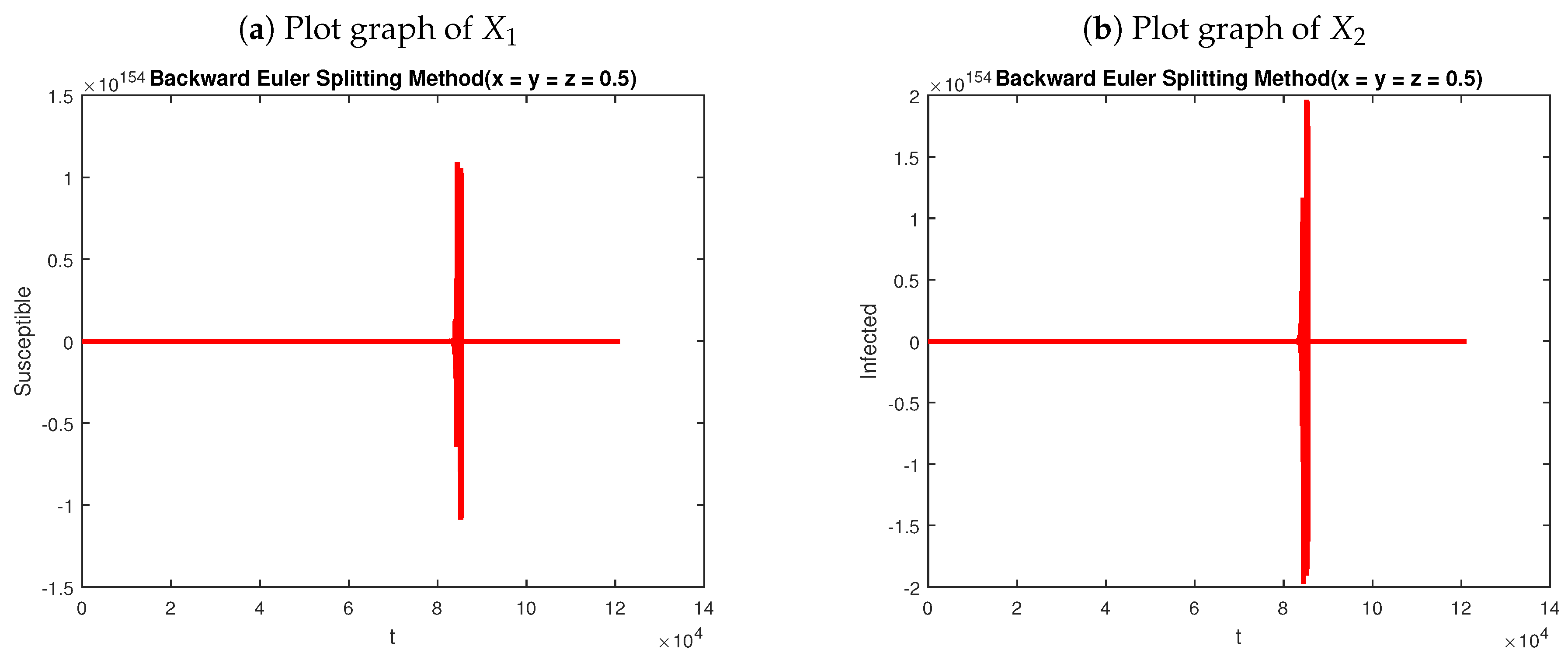
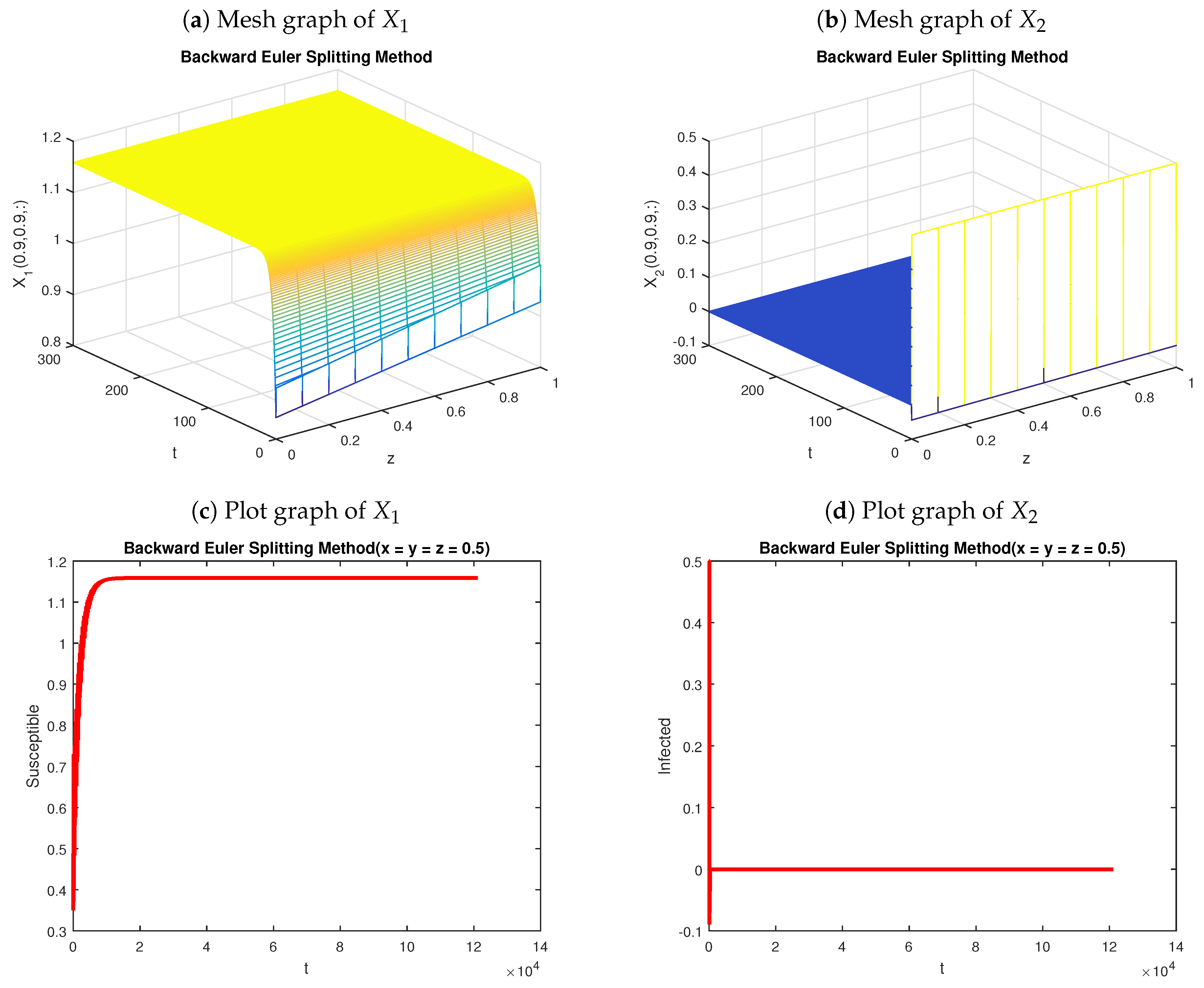
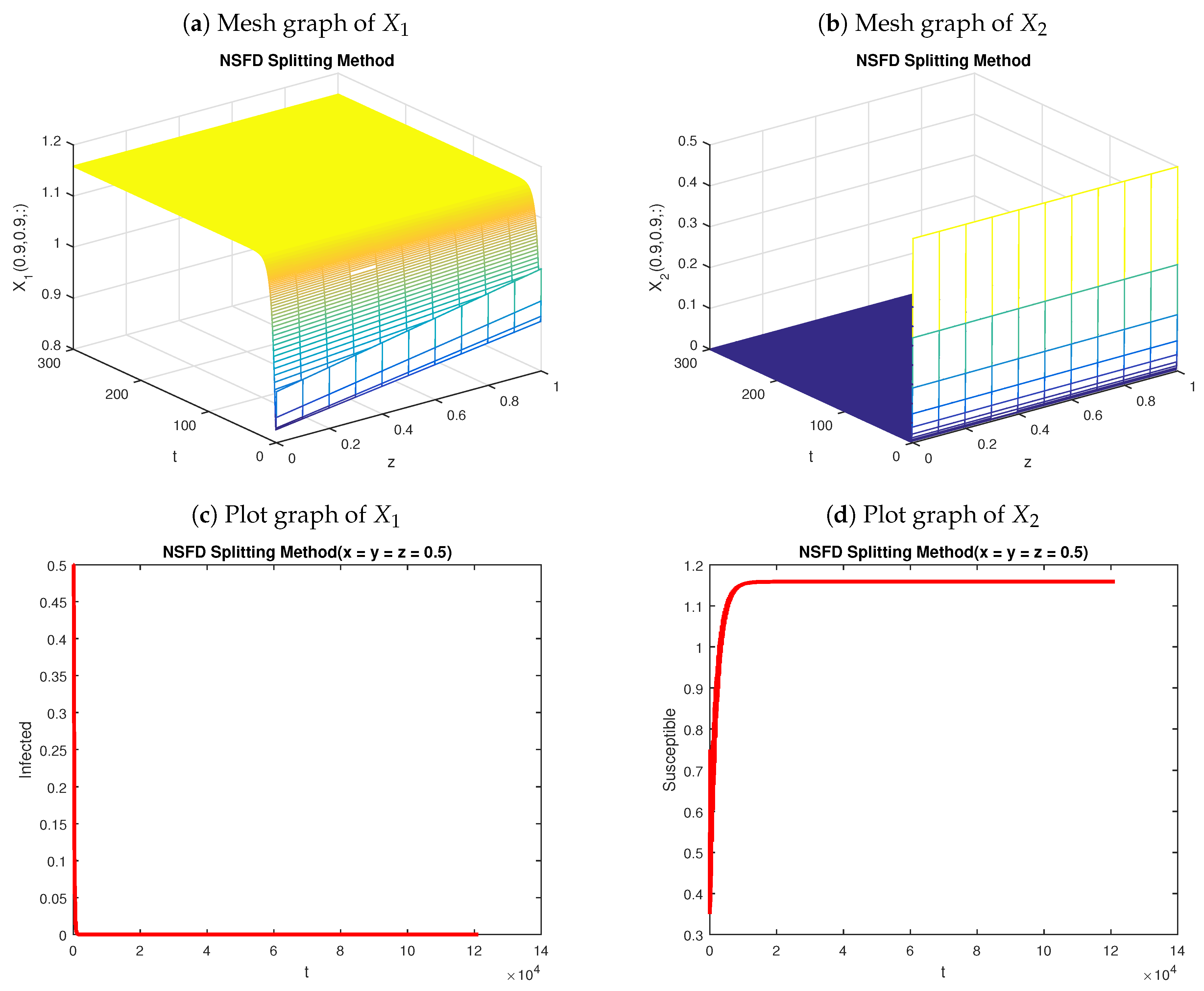
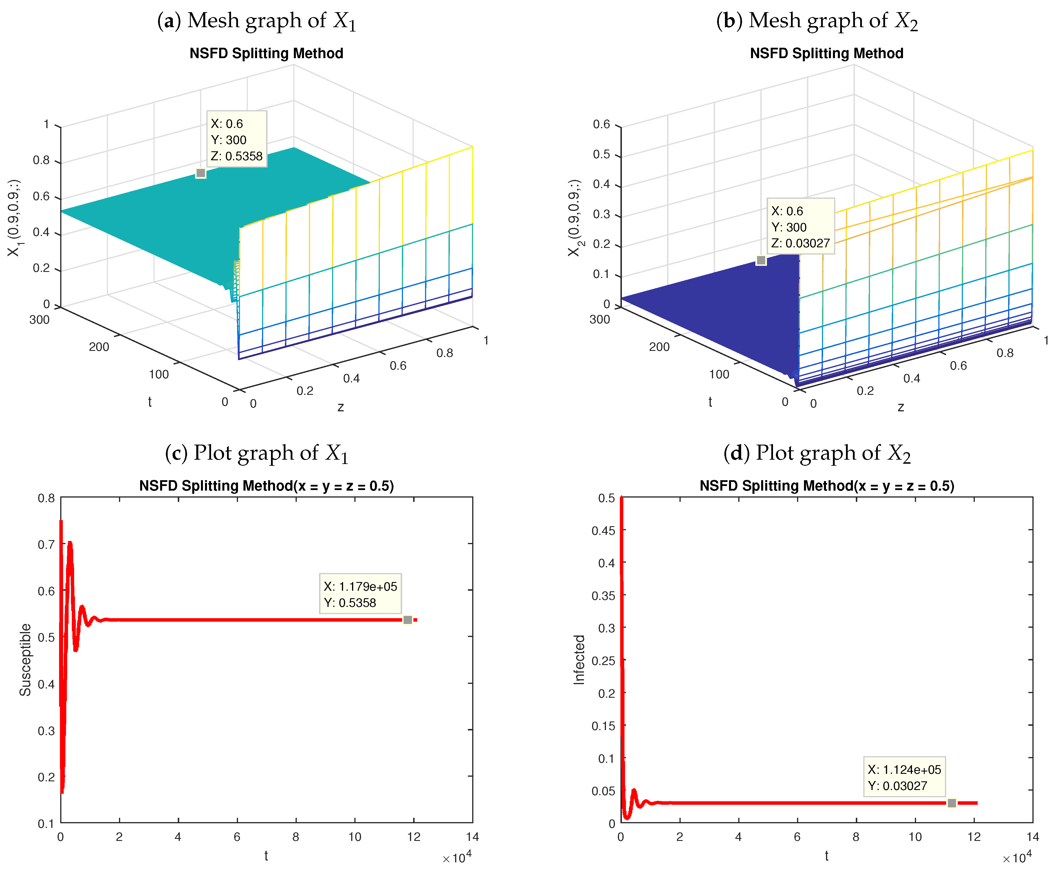
5. Computer Simulations

The purpose of this section is to provide some numerical examples to illustrate the performance of the schemes. Throughout, let $\lambda =0.232$, $\gamma =0.9$, $\nu =0.2$, $\beta =4.12$, ${\mu }_0=0.000232$, ${\mu }_1=0.0000547$, $d_1=0.001$ and $d_2=0.01$. We will consider the system (3) with initial conditions

$$\begin{array}{cc}\hfill {\rho }_1(x,y,z)& =0.7x+0.3y+0.1z,0\le x,y,z\le 1\hfill \end{array}$$

(56)

$$\begin{array}{cc}\hfill {\rho }_2(x,y,z)& =1/2,0\le x,y,z\le 1.\hfill \end{array}$$

(57)

Example 1

(Simulation for DFEP). Let $\alpha =0.97$ so that the reproductive value is $B_0=0.222154<1$. As $B_0<1$, the system converges to the DFEP ${\epsilon }_0=(\frac{\lambda }{({\mu }_0+\nu )},0)$. Figure 1 shows the numerical solution of the epidemic system (3) using the backward Euler splitting method. The graphs exhibit the fact that this method is incapable of preserving the nonnegative character of the solutions. In turn, Figure 2 shows the numerical solution of the model using the nonstandard finite-difference splitting method. The same values of parameters are used to obtain Figure 1 and Figure 2. Again, the results show that the second numerical scheme is capable of preserving the positivity of the solutions, as desired.

Example 2 (Simulation for FEP).

Let now $\alpha =7.9$. Notice that $B_0=2.22154>1$. In this case, the system (1) and (2) converges towards the EEP ${\epsilon }_{\ast }=(0.5358,0.03027)$. As we know, the backward Euler is stable and consistent, so convergent. However, Figure 3 shows that this method diverges. On the other hand, the nonstandard technique retains the structure of solutions of our continuous model. This is confirmed by Figure 4, which shows that that scheme preserves the stability of the EEP, along with the positivity of the solutions.

Before closing this section, we must recapitulate on the relevance of the numerical results presented in this work. To start with, various graphical results have been provided in the present stage. Among those results, possibly the most important ones are those in Figure 3 and Figure 4. Notice that the graphs of Figure 3 show that the backward Euler splitting method at EEP diverges in the long term. Indeed, notice that both $X_1$ and $X_2$ blow up after $t=8\times {10}^4$. It is well known that the backward Euler splitting scheme is unconditionally stable and consistent, so convergent. However, for the present nonlinear model, this scheme is incapable of preserving the actual behavior of the continuous model. These graphs demonstrate that the backward Euler operator splitting method fails to preserve the stability of the EEP for the give parameter values. On the contrary, Figure 4 shows that the nonstandard approach is actually capable of preserving the stability of the EEP. This confirms that the latter scheme is a dynamically consistent discretization of the model under investigation.

6. Conclusions

In this work, we investigated numerically a susceptible-infected-recovered hepatitis B epidemic reaction-diffusion model in three spatial dimensions. The stability and bifurcation analysis of the continuous model was rigorously discussed in this work. To study the dynamics of this system, we proposed a structure-preserving nonstandard finite-difference splitting numerical method. The scheme is capable of preserving all the important features of the continuous system like the positivity and the stability of steady states. To verify our results, comparisons were made against a classical backward Euler splitting method. Some numerical tests were conducted using both splitting methods, and we confirmed that the nonstandard scheme is dynamically consistent with the nonlinear model [44,45,46]. On the contrary, the backward Euler splitting method is incapable of preserving the positivity and the stability of the steady states.

The present manuscript provides a comparative numerical study between the backward Euler splitting method and a nonstandard finite-difference splitting numerical method. As far as numerical modeling for three-dimensional reaction-diffusion epidemic systems is concerned, very little research work can be found in the literature. Moreover, to the best of our knowledge and information, the literature lacks sufficient reports on structure-preserving numerical methods to solve three-dimensional epidemic models. Nevertheless, the present work proposes a structure-preserving scheme to solve a general three-dimensional diffusive model with time evolution. The proposed model provides a realistic approach in the sense that it considers non-homogeneous populations. Furthermore, to the best of our knowledge, the stability of the equilibrium point for the system under investigation is tackled herein for the first time in the literature.

References

1. Yuen, M.F.; Chen, D.S.; Dusheiko, G.M.; Janssen, H.L.; Lau, D.T.; Locarnini, S.A.; Peters, M.G.; Lai, C.L. Hepatitis B virus infection. Nat. Rev. Dis. Prim. 2018, 4, 18035. [Google Scholar] [CrossRef]
2. Tedder, R.; Zuckerman, M.; Brink, N.; Goldstone, A.; Fielding, A.; Blair, S.; Patterson, K.; Hawkins, A.; Gormon, A.; Heptonstall, J.; et al. Hepatitis B transmission from contaminated cryopreservation tank. Lancet 1995, 346, 137–140. [Google Scholar] [CrossRef]
3. Jonas, M.M. Hepatitis B and pregnancy: An underestimated issue. Liver Int. 2009, 29, 133–139. [Google Scholar] [CrossRef]
4. Terrault, N.A.; Lok, A.S.; McMahon, B.J.; Chang, K.M.; Hwang, J.P.; Jonas, M.M.; Brown, R.S.; Bzowej, N.H.; Wong, J.B. Update on prevention, diagnosis, and treatment of chronic hepatitis B: AASLD 2018 hepatitis B guidance. Hepatology 2018, 67, 1560–1599. [Google Scholar] [CrossRef] [PubMed]
5. Sarin, S.; Kumar, M.; Lau, G.; Abbas, Z.; Chan, H.; Chen, C.; Chen, D.; Chen, H.; Chen, P.; Chien, R.; et al. Asian-Pacific clinical practice guidelines on the management of hepatitis B: A 2015 update. Hepatol. Int. 2016, 10, 1–98. [Google Scholar] [CrossRef] [PubMed]
6. CDC. Progress in hepatitis B prevention through universal infant vaccination–China, 1997–2006. MMWR Morb. Mortal. Wkly. Rep. 2007, 56, 441–445. [Google Scholar]
7. Lavanchy, D.; Kane, M. Global epidemiology of hepatitis B virus infection. In Hepatitis B Virus in Human Diseases; Springer: Berlin, Germany, 2016; pp. 187–203. [Google Scholar]
8. Mantzoukis, K.; Rodríguez-Perálvarez, M.; Buzzetti, E.; Thorburn, D.; Davidson, B.R.; Tsochatzis, E.; Gurusamy, K.S. Pharmacological interventions for acute hepatitis B infection. Cochrane Database Syst. Rev. 2017, 3, CD011645. [Google Scholar] [CrossRef]
9. Milner, B.P.; Wang, J. Acute Hepatitis B Viral Infection in a Patient with Common Variable Immunodeficiency: A Case Report: 2448. Am. J. Gastroenterol. 2018, 113, S1362. [Google Scholar] [CrossRef]
10. Chang, M.H. Hepatitis B virus infection. In Seminars in Fetal and Neonatal Medicine; Elsevier: New York, NY, USA, 2007; Volume 12, pp. 160–167. [Google Scholar]
11. Terrault, N.A.; Bzowej, N.H.; Chang, K.M.; Hwang, J.P.; Jonas, M.M.; Murad, M.H. A ASLD guidelines for treatment of chronic hepatitis B. Hepatology 2016, 63, 261–283. [Google Scholar] [CrossRef]
12. El-Serag, H.B. Epidemiology of viral hepatitis and hepatocellular carcinoma. Gastroenterology 2012, 142, 1264–1273. [Google Scholar] [CrossRef]
13. Safi, M.A. Global Stability Analysis of Two-Stage Quarantine-Isolation Model with Holling Type II Incidence Function. Mathematics 2019, 7, 350. [Google Scholar] [CrossRef]
14. Nistal, R.; De la Sen, M.; Alonso-Quesada, S.; Ibeas, A. On a new discrete SEIADR model with mixed controls: Study of its properties. Mathematics 2019, 7, 18. [Google Scholar] [CrossRef]
15. Abouelkheir, I.; Kihal, F.E.; Rachik, M.; Elmouki, I. Optimal Impulse Vaccination Approach for an SIR Control Model with Short-Term Immunity. Mathematics 2019, 7, 420. [Google Scholar] [CrossRef]
16. Liu, X.L.; Pan, S. Spreading speed in a nonmonotone equation with dispersal and delay. Mathematics 2019, 7, 291. [Google Scholar] [CrossRef]
17. Mann, J.; Roberts, M. Modelling the epidemiology of hepatitis B in New Zealand. J. Theor. Biol. 2011, 269, 266–272. [Google Scholar] [CrossRef] [PubMed]
18. Tilahun, G.T.; Makinde, O.D.; Malonza, D. Co-dynamics of pneumonia and typhoid fever diseases with cost effective optimal control analysis. Appl. Math. Comput. 2018, 316, 438–459. [Google Scholar] [CrossRef]
19. Martin, N.K.; Vickerman, P.; Hickman, M. Mathematical modelling of hepatitis C treatment for injecting drug users. J. Theor. Biol. 2011, 274, 58–66. [Google Scholar] [CrossRef]
20. Lemos-Paião, A.P.; Silva, C.J.; Torres, D.F. An epidemic model for cholera with optimal control treatment. J. Comput. Appl. Math. 2017, 318, 168–180. [Google Scholar] [CrossRef]
21. White, M.T.; Verity, R.; Churcher, T.S.; Ghani, A.C. Vaccine approaches to malaria control and elimination: Insights from mathematical models. Vaccine 2015, 33, 7544–7550. [Google Scholar] [CrossRef]
22. Agusto, F.; Bewick, S.; Fagan, W. Mathematical model for Zika virus dynamics with sexual transmission route. Ecol. Complex. 2017, 29, 61–81. [Google Scholar] [CrossRef]
23. Cheng, Q.; Jing, Q.; Spear, R.C.; Marshall, J.M.; Yang, Z.; Gong, P. Climate and the timing of imported cases as determinants of the dengue outbreak in Guangzhou, 2014: Evidence from a mathematical model. PLoS Neglect. Trop. Dis. 2016, 10, e0004417. [Google Scholar] [CrossRef] [PubMed]
24. Parham, P.E.; Waldock, J.; Christophides, G.K.; Hemming, D.; Agusto, F.; Evans, K.J.; Fefferman, N.; Gaff, H.; Gumel, A.; LaDeau, S.; et al. Climate, environmental and socio-economic change: Weighing up the balance in vector-borne disease transmission. Philos. Trans. R. Soc. B Biol. Sci. 2015, 370, 20130551. [Google Scholar] [CrossRef] [PubMed]
25. Medlock, J.; Kot, M. Spreading disease: Integro-differential equations old and new. Math. Biosci. 2003, 184, 201–222. [Google Scholar] [CrossRef]
26. Khan, T.; Zaman, G. Classification of different Hepatitis B infected individuals with saturated incidence rate. SpringerPlus 2016, 5, 1082. [Google Scholar] [CrossRef] [PubMed]
27. Parsamanesh, M.; Erfanian, M. Global dynamics of an epidemic model with standard incidence rate and vaccination strategy. Chaos Solitons Fractals 2018, 117, 192–199. [Google Scholar] [CrossRef]
28. Ahmed, N.; Shahid, N.; Iqbal, Z.; Jawaz, M.; Rafiq, M.; Tahira, S.; Ahmad, M. Numerical Modeling of SEIQV Epidemic Model with Saturated Incidence Rate. J. Appl. Environ. Biol. Sci. 2018, 8, 67–82. [Google Scholar]
29. Khan, T.; Ullah, Z.; Ali, N.; Zaman, G. Modeling and control of the hepatitis B virus spreading using an epidemic model. Chaos Solitons Fractals 2019, 124, 1–9. [Google Scholar] [CrossRef]
30. Ervin, V.J.; Macías-Díaz, J.E.; Ruiz-Ramírez, J. A positive and bounded finite element approximation of the generalized Burgers–Huxley equation. J. Math. Anal. Appl. 2015, 424, 1143–1160. [Google Scholar] [CrossRef]
31. Macías-Díaz, J.E.; Villa-Morales, J. A deterministic model for the distribution of the stopping time in a stochastic equation and its numerical solution. J. Comput. Appl. Math. 2017, 318, 93–106. [Google Scholar] [CrossRef]
32. Macías-Díaz, J.E.; Landry, R.; Puri, A. A finite-difference scheme in the computational modelling of a coupled substrate-biomass system. Int. J. Comput. Math. 2014, 91, 2199–2214. [Google Scholar] [CrossRef]
33. Ahmed, N.; Tahira, S.; Rafiq, M.; Rehman, M.; Ali, M.; Ahmad, M. Positivity preserving operator splitting nonstandard finite difference methods for SEIR reaction diffusion model. Open Math. 2019, 17, 313–330. [Google Scholar] [CrossRef]
34. Ahmed, N.; Rafiq, M.; Rehman, M.; Iqbal, M.; Ali, M. Numerical modeling of three dimensional Brusselator reaction diffusion system. AIP Adv. 2019, 9, 015205. [Google Scholar] [CrossRef]
35. Macías-Díaz, J.E.; Puri, A. An explicit positivity-preserving finite-difference scheme for the classical Fisher–Kolmogorov–Petrovsky–Piscounov equation. Appl. Math. Comput. 2012, 218, 5829–5837. [Google Scholar] [CrossRef]
36. Macías-Díaz, J.E. Sufficient conditions for the preservation of the boundedness in a numerical method for a physical model with transport memory and nonlinear damping. Comput. Phys. Commun. 2011, 182, 2471–2478. [Google Scholar] [CrossRef]
37. Macías-Díaz, J.E.; Puri, A. A boundedness-preserving finite-difference scheme for a damped nonlinear wave equation. Appl. Numer. Math. 2010, 60, 934–948. [Google Scholar] [CrossRef]
38. Tomasiello, S. A note on three numerical procedures to solve Volterra integrodifferential equations in structural analysis. Comput. Math. Appl. 2011, 62, 3183–3193. [Google Scholar] [CrossRef] [Green Version]
39. Tomasiello, S. Some remarks on a new DQ-based method for solving a class of Volterra integro-differential equations. Appl. Math. Comput. 2012, 219, 399–407. [Google Scholar] [CrossRef]
40. Mickens, R.E. Nonstandard Finite Difference Models of Differential Equations; World Scientific: Singerpore, 1994. [Google Scholar]
41. Fujimoto, T.; Ranade, R.R. Two characterizations of inverse-positive matrices: The Hawkins-Simon condition and the Le Chatelier-Braun principle. Electron. J. Linear Algebra 2004, 11, 6. [Google Scholar] [CrossRef] [Green Version]
42. Harwood, R.C.; Manoranjan, V.S.; Edwards, D.B. Lead-acid battery model under discharge with a fast splitting method. IEEE Trans. Energy Convers. 2011, 26, 1109–1117. [Google Scholar] [CrossRef]
43. Tian, G.X.; Huang, T.Z. Inequalities for the minimum eigenvalue of M-matrices. ELA Electron. J. Linear Algebra 2010, 20. [Google Scholar] [CrossRef]
44. Macías-Díaz, J.E. An explicit dissipation-preserving method for Riesz space-fractional nonlinear wave equations in multiple dimensions. Commun. Nonlinear Sci. Numer. Simul. 2018, 59, 67–87. [Google Scholar] [CrossRef]
45. Macías-Díaz, J.E. Numerical simulation of the nonlinear dynamics of harmonically driven Riesz-fractional extensions of the Fermi–Pasta–Ulam chains. Commun. Nonlinear Sci. Numer. Simul. 2018, 55, 248–264. [Google Scholar] [CrossRef]
46. Macías-Díaz, J.E. Numerical study of the transmission of energy in discrete arrays of sine-Gordon equations in two space dimensions. Phys. Rev. E 2008, 77, 016602. [Google Scholar] [CrossRef]
Figure 1. Graphs of backward Euler splitting method at DFEP with Δ x = 0.1 , ζ 1 = 0.1 and ζ 2 = 0.3 .
Mathematics 07 01157 g001
Figure 2. Graphs of the nonstandard finite-difference implicit splitting method at DFEP with Δ x = 0.1 , ζ 1 = 0.1 and ζ 2 = 0.3 .
Mathematics 07 01157 g002
Figure 3. Graphs of backward Euler splitting method at EEP with Δ x = 0.1 , ζ 1 = 0.1 and ζ 2 = 0.3 .
Mathematics 07 01157 g003
Figure 4. Graphs of nonstandard splitting method at EEP with Δ x = 0.1 , ζ 1 = 0.1 and ζ 2 = 0.3 .
Mathematics 07 01157 g004