Article

Inframarginal Model Analysis of the Evolution of Agricultural Division of Labor

1
College of Mathematics and Informatics, South China Agricultural University, Guangzhou 510642, China
2
Department of Mathematics and Statistics, California State University, Long Beach, CA 90840, USA
*
Author to whom correspondence should be addressed.
Mathematics 2019, 7(12), 1152; https://doi.org/10.3390/math7121152
Submission received: 24 October 2019 / Revised: 24 November 2019 / Accepted: 25 November 2019 / Published: 1 December 2019
(This article belongs to the Special Issue Mathematics and Engineering)

Abstract

:
Division of labor plays a critical role in many parts of agriculture. For example, a specialized division of labor can lead to the improvement of labor productivity, the reduction of production costs, and the innovation of production technology and organization. At the heart of agricultural management is how the comparative advantages of farmers impact their production decision-making behavior, and, consequently, influence the division of labor structure. In this paper, we apply an infra-marginal model to interpret the selection logic of heterogeneous farmers’ specialized production with exogenous comparative technical advantages and transaction costs. Solving the nonlinear programming problem of the utility function within each respective labor structure leads to a corner equilibrium. Under reasonable assumptions of the model, we reduced the number of possible production–consumption decision modes from the maximum of 64 to an optimal of 3. Through this analysis, we discovered the ranges for transaction efficiency coefficients and preference parameter under which each structure can achieve general equilibrium. Our theoretical model thereby explains the structural evolution of agricultural division of labor.

1. Introduction

In agriculture, each farmer behaves as a limited and rational production decision maker; farmers allocate resources rationally similar to entrepreneurs. In the traditional agriculture where profit maximization is the farmers’ ultimate behavioral goal, it is relatively rare to see an inefficient allocation of production factors [1]. As long as farmers prefer the principle of manufacturer in management, they may allocate resources to the most efficient production field, thus bringing specialization and division of labor. Specialized division of labor has a direct impact on economics that leads to the improvement of labor productivity and the reduction of production costs, and an indirect impact that leads to the innovation of production technology and organization. Together, these impacts lead to the saving of factor resources and the improvement of labor efficiency [2]. Under the appropriate external economic conditions, the development of the division of labor within the household will naturally devote labor and capital on a few business activities, or even one. As a result, farmers generally increase the amount of capital, technology, or land input in the original factor combination, forming an intensive management based on a certain factor. Therefore, the rational production decision of farmers is to pursue the division of labor economy formed by the comparative advantage.
China’s current policies focus on promoting moderate scale and specialized agricultural operation to improve the scale economy and division of labor economy, and promoting the transformation of agricultural management methods. An underlying aspect of such policies is to encourage farmers to switch from small and full to specialized management. The heterogeneity of the farmers is assumed in the heart of agricultural management. That is, the farmers have their own comparative advantages under the conditions of open management. With this assumption, we study the effect of the comparative advantages on the production decision-making behavior, which then influences the kind of division of labor structure we present. This forms the basis of our paper.
Our study uses the Ricardian model [3,4,5] to include the comparative advantages of farmers and market transaction costs. David Ricardo’s theory of comparative advantage is considered the cornerstone of modern trade theory. However, due to the presence of corner solutions, traditional marginal analysis cannot be applied to the Ricardo model [6]. For this reason, the model has not received its due attention [4]. If we used the absolute separation between pure consumers and enterprises, we would generate multiple general equilibria based on multiple corner and interior point solution structures. However, under the Walras system, companies do not care which structure they choose, and pure consumers cannot choose the production structure. Hence, partial equilibrium may be a general equilibrium in each structure. This multiplicity of the general equilibrium makes comparatively static analysis of general equilibrium impossible [7]. Now, if the Smith framework is used for analysis, each individual can be a producer–consumer, and can choose its level of specialization. That is, the general equilibrium is one of the multiple corner equilibria. The general equilibrium is an effective compromise between the division of labor economies generated by exogenous comparative technological advantages and transaction costs [6].
In the literature, there are exogenous and endogenous comparative advantages, as well as comprehensive comparative advantages [8,9,10]. Based on the Ricardo model, we construct a mathematical model on farmers’ participation in the division of labor with exogenous comparative technical advantages and transaction costs by taking into consideration the simplification of the model and the simplicity of the structure. In our work, we pioneer the use of the infra-marginal model to study the evolution of agricultural division of labor, which is about farmers’ specialization and the change of their agricultural economic organization.
The infra-marginal model provides a powerful tool to study the division of labor and professionalization of the economy. The concept was initiated in the 1950s and 1960s [11,12,13] and further developed by Yang [14,15]. In such a model, it is assumed that business decisions can be categorized into two classes: marginal and infra-marginal. Marginal decisions are concerned with the extent to which resources are allocated to a pre-determined set of activities, while infra-marginal decisions are about what activities to engage in (or whether or not to engage in an activity). In the context of social division of labor, the infra-marginal decisions of individuals allow the formation of a network division of labor of various sizes. The infra-marginal analysis is concerned with the optimal infra-marginal network decisions and the outcome of these decisions. The optimal infra-marginal network decisions rely on the total cost–benefit analysis across different network patterns of specialization and trade connections as well as the marginal analysis of resource allocation for a given network pattern. Mathematically speaking, infra-marginal analysis transcends into non-classical mathematical programming problems (e.g., linear and nonlinear programming, mixed integer programming, dynamic programming, and control theory) that allow corner solutions [16].
The infra-marginal model finds a variety of applications. For example, it can be coupled with the Ricardian model to study the mechanisms for economic development as well as the evolution of trade policy regimes [3,4,5,17]. Infra-marginal analysis was applied to the Dixit–Krugman model to explain the evolution of trade pattern determined by the interplay between endogenous and exogenous comparative advantages [18]. It was also used in the Dixit–Stiglitz model to predict the tests of scale effects [19]. The aforementioned applications are all on international trade. Moreover, dynamic infra-marginal analysis was applied in the Yang and Borland (Y–B) model to obtain the dynamic general equilibrium based on corner solutions. It can also be seen in the areas of economic growth and development theory [8,20]. More applications of the infra-marginal model can be found in the studies of the firm, contract and property rights, insurance, e-business, money, capital and business cycle [21,22,23,24,25,26,27], and urbanization and industrialization such as the relationships among the division of labor, agglomeration, and land rentals [28,29]. Despite the rich applications of the infra-marginal model, its application to the special topic of agricultural division of labor is generally lacking. A major contribution of our work is the development of a framework that helps to explain the selection logic of farmers’ specialized production and the structural evolution of agricultural division of labor through the construction of an infra-marginal model.
The rest of the paper is organized as follows. In Section 2, we construct an infra-marginal model by considering agricultural comparative advantages. The model consists of four possible division of labor structures. In Section 3, we set up and develop the corner equilibrium solutions to the nonlinear utility optimization problems that are associated with the four structures. In Section 4, we analyze the conditions in the parameter space that lead to various general equilibria as well as explain the division selection logic and decision mechanism of farmers with comparative advantage. We conclude our work with a summary and discussion in Section 5.

2. Materials and Methods—An Infra-Marginal Model

Based on the Ricardo model with exogenous comparative technical advantages and transaction cost, we construct an infra-marginal model of farmers’ comparative advantage and specialization choice, which reveals the selection logic of farmers’ specialized production and the structural evolution rule of agricultural division of labor.

2.1. Model Definition

Our mathematical model inherits a set of reasonable assumptions. The economy is composed of two producer–consumer integrated farmers and each farmer has a comparative advantage due to their heterogeneity. Two different farmers, Farmers 1 and 2, both consume two agricultural products x and y (x and y may also be labor services in agricultural production links) and determine their own patterns of production and trading activities.
With these assumptions, the farmer production system (as a production–consumer integration in the model) can be constructed. In general, we have at our disposal many utility functions (e.g., linear, Leontief, constant elasticity substitution, Cobb–Douglas (C-D), etc.). Each comes with a set of restrictions. In our agricultural model, the two labor services or products are both necessary and indispensable to the final product. This assumption is enforced with a zero utility if one of the necessary services or products has a value of zero. Since C-D utility function is the only one among those described above that satisfies this requirement, it is used in our model.
The utility function of farmer i ( i = 1 , 2 ) is:
U i = ( x i + k x i d ) β ( y i + k y i d ) 1 β ,
where x i and y i are the respective self-sufficiency quantities of agricultural products (or production link), x i d and y i d are the respective demand quantities of farmers, k is the transaction efficiency coefficient, and β is the preference parameter of farmers.
The production functions of farmer i ( i = 1 , 2 ) are:
x i p = x i + x i s = a i x l i x , and y i p = y i + y i s = a i y l i y .
Here, x i p and y i p are, respectively, the output level of two kinds of agricultural products produced by farmers (or labor services engaged in two production links); and x i s and y i s are, respectively, the supply quantity of farmers’ products or labor service. Moreover, l i j ( i = 1 , 2 ; j = x , y ) is the amount of labor used by farmer i to produce agricultural product (or labor services) j, which is called the level of specialization of farmer i when producing agricultural product (or labor services) j. In addition, coefficient a i j is the labor productivity of farmer i when producing agricultural product (or labor services) j.
Under these definitions, the case where Farmer 1 has a comparative advantage in the production of agricultural product (or labor services) x can be represented mathematically by a 1 x / a 1 y > a 2 x / a 2 y . It means that, compared to Farmer 2, Farmer 1 has a higher relative productivity on x over y; therefore, Farmer 1’s opportunity cost for product x is smaller.
Moreover, we can use the labor endowment constraint to measure farmers’ level of specialization. In particular, the labor endowment constraint of farmer i is given by l i x + l i y = 1 . For example, l i x = 0 means that farmer i devotes all of their labor to produce product y, making them a specialized producer of y.
Farmers’ consumption, production, and trading decisions involve six non-negative variables x i , x i s , x i d , y i , y i s , and y i d , resulting in a total of 2 6 = 64 combinations.
With market clearing (supply equals demand), the budget constraint reads p x x i s + p y y i s = p x x i d + p y y i d . To avoid needless trade cost, it is prohibited to buy and sell the same product (or service). As a result, x i s and x i d cannot be positive at the same time, i.e., x i s x i d = 0 . The same holds true for product y to arrive at y i s y i d = 0 . Overall, the budget constraint simplifies to ( y i s = x i d = 0 , p x x i s = p y y i d ) or ( x i s = y i d = 0 , p x x i d = p y y i s ) .

2.2. Optimal Decision Mode and Division of Labor Structure

Based on the budget constraint and the other constraints that we present next, most of the optimal decisions from the 64 possible combinations can be excluded. Consequently, only a few division of labor structures are deduced. In all cases, any combination of the six variables should meet the budget constraints and the condition of positive utility.
For the convenience of the analysis, we write the variables into a 6-tuple Z i = ( x i , x i s , x i d , y i , y i s , y i d ) . We use the notations 0 or + inside the 6-tuple to denote zero or positive values. For example, ( , 0 , + , , , ) denotes the case x i s = 0 and x i d > 0 . The cases that violate budget constraint are: ( , 0 , , , , + ) , ( , + , , , , 0 ) , ( , , 0 , , + , ) , and ( , , + , , 0 , ) . There are a total of 2 4 + 2 3 + 2 4 + 2 3 = 48 such combinations. Moreover, there are four cases with ( , + , + , , + , + ) that involve selling and buying the same product, which are inefficient cases, because they introduce unnecessary transaction costs. In the remaining 12 combinations, there are seven combinations with either the form ( 0 , , 0 , , , ) or ( , , , 0 , , 0 ) , which do not meet the positive utility constraint U i > 0 . The remaining five cases can be summarized into three decision modes: self-sufficient mode ( + , 0 , 0 , + , 0 , 0 ) , semi-specialized mode ( ( + , + , 0 , + , 0 , + ) and ( + , 0 , + , + , + , 0 ) ), and complete-specialization mode ( ( + , + , 0 , 0 , 0 , + ) and ( 0 , 0 , + , + , + , 0 ) ). These three decision modes are assigned to Farmer 1 or Farmer 2. We call a combination of modes for both farmers a structure. With the comparative advantage assumption of Farmer 1 producing product x, certain structures need to be avoided. For example, the structures with either Z 1 = ( 0 , 0 , + , + , + , 0 ) (meaning Farmer 1 specializes in production y) or Z 2 = ( + , + , 0 , 0 , 0 , + ) (meaning Farmer 2 specializes in production x) violate the comparative disadvantage of individual farmers, hence need to be excluded from consideration. Now, we analyze in detail the three modes that make up the various types of structures.
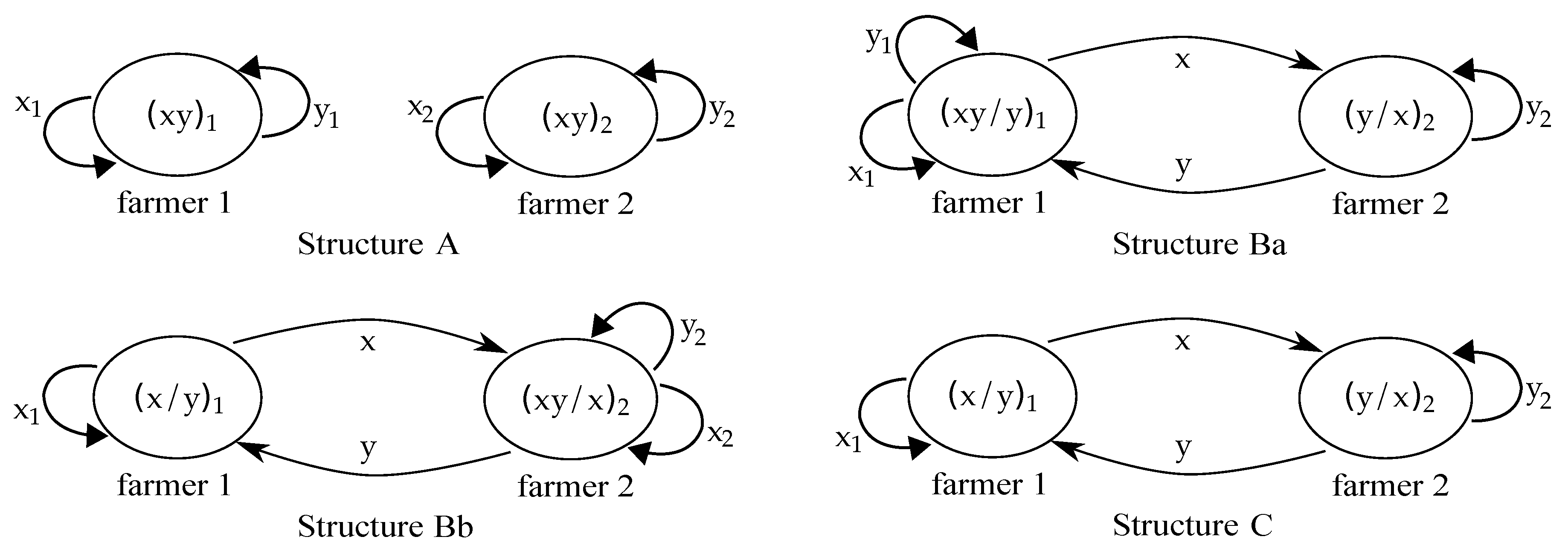
  • Self-sufficiency mode is generally expressed as ( x y ) i and defined as Z i = ( + , 0 , 0 , + , 0 , 0 ) , for i = 1 , 2 . This indicates that all agricultural products or labor services are self-sufficient. With an economy of two farmers, this kind of social organization structure is called self-sufficiency Structure A.
  • Semi-specialized mode is when farmers produce products or services with comparative advantages, generally expressed as ( x y / y ) 1 and ( x y / x ) 2 . The mode ( x y / y ) 1 corresponds to the case where Z 1 = ( + , + , 0 , + , 0 , + ) , meaning that Farmer 1 produces certain self-sufficient quantities of products x and y, sells products x, and purchases products y. Consider the example of the labor of plant protection and weeding in agricultural production. Farmer 1 purchases a small portable spraying machine to spray chemicals on his own and others’ crops and he takes care of his own weeding partially. In addition, he also purchases weeding labor services from other farmers. Namely, he outsources the labor services of weeding. The mode ( x y / x ) 2 corresponds similarly to Z 2 = ( + , 0 , + , + , + , 0 ) .
  • Complete-specialization mode is when farmers produce products or services with comparative advantage, expressed as ( x / y ) 1 and ( y / x ) 2 . The mode ( x / y ) 1 , or Z 1 = ( + , + , 0 , 0 , 0 , + ) , represents the case where Farmer 1 specializes in producing goods or services x and is self-sufficient in selling x and buying goods or services y. The mode ( y / x ) 2 , or Z 2 = ( 0 , 0 , + , + , + , 0 ) , represents that Farmer 2 specializes in producing goods or services y and is self-sufficient in selling y and buying goods or services x.
In addition to self-sufficiency Structure A, the decisions of Farmers 1 and 2 to their own production and trading activities also involve two partial division of labor structures: Ba, composed of ( x y / y ) 1 and ( y / x ) 2 ; Bb, composed of ( x / y ) 1 and ( x y / x ) 2 ; and a complete division of labor Structure C, which is composed of ( x / y ) 1 and ( y / x ) 2 . The above modes and structures are demonstrated in Figure 1.

3. Optimization Analysis—Decision and Corner Equilibrium

To analyze the comparative advantages of exogenous technology of farmers and how the transaction costs affect the division of labor, that is, how the social organization structure evolves from self-sufficiency to partial division of labor and then to complete division of labor, it is necessary to analyze the decision-making strategies by first maximizing individual utility based on the infra-margin, to obtain partial or corner equilibriums for each given structure. The general equilibrium is one of the four corner equilibria with the maximum utility. To do this, we first use nonlinear programming to solve the problem of maximization of farmers’ individual benefits, then use the market clearing conditions to solve the partial equilibrium of each of the four structures, and finally use the total return-cost analysis method to determine the general equilibrium.

3.1. The Selection of Self-Sufficiency Mode

The selection of self-sufficiency mode ( x y ) 1 can be formulated as:
max x 1 , y 1 , l 1 x , l 1 y U 1 = x 1 β y 1 1 β
s . t . x 1 = a 1 x l 1 x , y 1 = a 1 y l 1 y , l 1 x + l 1 y = 1
We use the marginal analysis method to solve this problem by first substituting the constraints into the objective function, and then setting the first derivative to zero. This yields the solution l 1 x = β , l 1 y = 1 β , x 1 = a 1 x β , y 1 = a 1 y ( 1 β ) , with the utility of self-sufficient Farmer 1 being U A 1 = β β ( 1 β ) 1 β a 1 x β a 1 y 1 β . Similarly, the utility of self-sufficient Farmer 2 is U A 2 = β β ( 1 β ) 1 β a 2 x β a 2 y 1 β .

3.2. The Selection of Semi-Specialized Mode

Given the partial division of labor Structure Ba, the utility maximization problem for semi-specialized mode ( x y / y ) 1 is:
max x 1 , y 1 , x 1 s , y 1 d , l 1 x , l 1 y U 1 = x 1 β ( y 1 + k y 1 d ) 1 β
s . t . x 1 + x 1 s = a 1 x l 1 x , y 1 = a 1 y l 1 y , l 1 x + l 1 y = 1 , y 1 d = p x 1 s ,
where p p x / p y is the relative price of product or service x compared to y. Similarly, to solve this problem, we substitute all the variables in the objective function with l 1 x and x 1 s using the four constraints. The first-order derivatives are
U 1 x 1 s = β a 1 x l 1 x x 1 s + k p ( 1 β ) a 1 y ( 1 l 1 x ) + k p x 1 s U 1
U 1 l 1 x = a 1 x β a 1 x l 1 x x 1 s a 1 y ( 1 β ) a 1 y ( 1 l 1 x ) + k p x 1 s U 1
Setting both derivatives zero then requires p = a 1 y / ( k a 1 x ) . It then follows naturally that x 1 = β a 1 x , x 1 s = a 1 x ( l 1 x β ) , y 1 = a 1 y ( 1 l 1 x ) , y 1 d = a 1 y ( l 1 x β ) / k , and U 1 = β β ( 1 β ) 1 β a 1 x β a 1 y 1 β . We refer the interested reader to Appendix A.1 for more details. Interestingly, the maximizer variables x 1 s , y 1 , and y 1 d are functions of l 1 x , while the maximal utility U 1 is independent of l 1 x . The above equilibrium solution relies on a fixed relative market price p. Our analysis in the following remarks shows that this relative market price determines the mode choice of Farmer 1.
Remark 1.
If p > a 1 y / ( k a 1 x ) , with the optimal value of x 1 s given by U 1 / x 1 s = 0 , we have U 1 / l 1 x > 0 . This means the utility of Farmer 1 can always be improved by improving l 1 x . That is, the utility of Farmer 1 will always increase with the increase of labor allocation to x (the specialization level generating x). Therefore, the optimal value of l 1 x is its upper limit value. Due to the constraint of farmers’ endowment of working hours, if the upper limit l 1 x = 1 is taken, the farmer should not produce y, but should be specialized in the production of x. That is, when p > a 1 y / ( k a 1 x ) , Farmer 1 will choose the mode ( x / y ) 1 instead of the mode ( x y / y ) 1 . Similarly, when p < a 1 y / ( k a 1 x ) , Farmer 1 will choose the mode ( x y ) 1 instead of the mode ( x y / y ) 1 . Only when the relative price of market p is a 1 y / ( k a 1 x ) will Farmer 1 select mode ( x y / y ) 1 . This condition is similar to the zero-profit condition in the standard general equilibrium with the same scale return.
Remark 2.
It is seen that, if the relative price p of the transaction cost, after any discount, in the market is lower than the marginal conversion rate a 1 y / ( k a 1 x ) of Farmer 1 in self-sufficiency, the optimal decision of farmers is to be self-sufficient and produce two products or services x and y at the same time. If p > a 1 y / ( k a 1 x ) , the marginal utility of the level of specialization of the Farmer 1 always increases with the increase of l 1 x , so the optimal decision is to specialize in producing x. However, when p is a 1 y / ( k a 1 x ) , self-sufficiency mode and semi-specialized mode ( x y / y ) 1 produce the same effect. Thus, if the market clearing conditions in the general equilibrium can ensure that demand and supply can be achieved in mode ( x y / y ) 1 , the farmer will choose this mode. In this decision-making solution, the optimal value of l 1 x is uncertain, and its equilibrium value will be determined by the conditions for market clearing.

3.3. The Selection of Complete-Specialized Mode

The utility maximization problem for Farmer 2 with mode ( y / x ) 2 is:
max x 2 d , y 2 , y 2 s U 2 = ( k x 2 d ) β y 2 1 β
s . t . y 2 + y 2 s = a 2 y l 2 y , y 2 s = p x 2 d , l 2 y = 1 .
In the context of Structure Ba, ( y / x ) 2 is selected jointly with ( x y / y ) 1 , and p = a 1 y / ( k a 1 x ) is the equilibrium relative price. The system yields the optimal solution x 2 d = k β a 2 y a 1 x / a 1 y , y 2 = ( 1 β ) a 2 y , y 2 s = β a 2 y . The market clearing conditions x 1 s = x 2 d lead to l 1 x = β + k β a 2 y / a 1 y . The condition l 1 x < 1 is met if and only if a 2 y / a 1 y < ( 1 β ) / ( k β ) , in which case Structure Ba is selected. At this point, the maximum utility of Farmer 2, that is, the real income per capita, is U 2 = β β ( 1 β ) 1 β ( k 2 a 1 x / a 1 y ) β a 2 y .
In the context of Structure C, the maximization utility problem for Farmer 1 with mode ( x / y ) 1 is:
max x 1 , x 1 s , y 1 d U 1 = x 1 β ( k y 1 d ) 1 β ,
s . t . x 1 + x 1 s = a 1 x l 1 x , y 1 d = p x 1 s , l 1 x = 1 ,
with solution x 1 = β a 1 x , x 1 s = ( 1 β ) a 1 x , and y 1 d = ( 1 β ) p a 1 x . Similarly, we can establish the maximization problem for Farmer 2 with mode ( y / x ) 2 . The market clearing condition x 1 s = x 2 d sets the equilibrium relative price p = β a 2 y ( 1 β ) a 1 x . Under this condition, the maximum utility of Farmer 1 in Structure C is U 1 c = β a 1 x β ( k a 2 y ) 1 β and the maximum utility of Farmer 2 is U 2 c = ( 1 β ) ( k a 1 x ) β a 2 y 1 β . For more details about the derivation, see Appendix A.2.
The comparative advantage of farmers and the equilibrium of four corner points in the model of division of labor selection are summarized in Table 1.

4. Selection Logic and Structural Evolution of Division of Labor

If heterogeneous farmers have exogenous comparative technical advantages, under the influence of market transaction cost, the choice of production and consumption will be made in the four division of labor structures listed above. As each of the four division of labor structures leads to a corner equilibrium (cf. Table 1), general equilibrium is among the corner equilibria. Under this corner equilibrium relative price, no farmer has incentive to deviate from the model he/she chooses. To explore the influence of comparative advantage and transaction cost on the division of labor choice of farmers, we find the conditions for each division of labor structure that lead to the general equilibrium. This can be accomplished using the total cost–benefit analysis method and the definition of general equilibrium. Furthermore, by studying the relationship between comparative advantage and transaction efficiency coefficient, we can deduce the varying relationships in farmers’ equilibrium in their division of labor. These analyses help explain the division selection logic and decision mechanism of farmers with comparative advantage.

4.1. General Equilibrium and Comparative Static Analysis

Let us take the partial division of labor Structure Ba as an example. If the following conditions are met, Structure Ba is a general equilibrium.
  • With the corner equilibrium relative price p = a 1 y / ( k a 1 x ) for this structure, Farmer 2 prefers ( y / x ) 2 , rather than mode ( x y ) 2 or ( x / y ) 2 , given that: (1) U 2 ( y / x ) > U 2 ( A ) , which is equivalent to k > k 0 = a 2 x a 1 y / a 1 x a 2 y ; and (2) U 2 ( y / x ) > U 2 ( x / y ) , which is equivalent to k > k 3 = a 2 x a 1 y / a 1 x a 2 y 2 β .
  • Farmer 1 prefers mode ( x y / y ) 1 than any other mode. This requires: (1) U 1 ( x y / x ) > U 1 ( x / y ) , which is true if a 1 y / a 1 x > k p ; and (2) U 1 ( x y / x ) > U 1 ( y / x ) , which is true if k < 1 .
  • Farmers are semi-specialized rather than fully specialized in producing products or services. This requires l 1 x < 1 , which is equivalent to k < k 1 = ( 1 β ) a 1 y / ( β a 2 y ) .
Notice that k 3 < k 0 and k 0 < k 1 are true if and only if ( 1 β ) / β > a 2 x a 1 y / a 1 x a 2 y . Hence, when k ( k 0 , k 1 ) , the three conditions above are true, and the corner equilibrium in Structure Ba is the general equilibrium. In this case, although Farmer 1 has an exogenous technological comparative advantage in the production of product or service x, he is unwilling to give up production of product or service y, because his relative preference for product or service y is greater than a threshold, which is the square root of the reciprocal of comparative advantage. Meanwhile, farmers are faced with a low market transaction efficiency coefficient, that is, farmers need to pay higher transaction costs to purchase the products or services they need, which sets farmers’ preference to produce a part of their own products or services. The comparative static analysis for other structures (A, Bb, and C) can be carried out in a similar way, which is summarized in Table 2 with
k 0 = a 2 x a 1 y / a 1 x a 2 y , k 1 = ( 1 β ) a 1 y / β a 2 y , and k 2 = β a 2 x / ( 1 β ) a 1 x .

4.2. The Logic and Decision Mechanism of Farmers Participating in the Division of Labor

Comparing various structures in the corresponding parameter subspace, as shown in Table 2, we can obtain relevant conclusions about the division of labor selection logic and decision mechanism of farmers with comparative advantages. In summary:
  • If k < k 0 (k is the transaction efficiency coefficient between farmers), the general equilibrium structure is self-sufficient, and the farmers produce two products or services themselves.
  • If k > k 0 and ( 1 β ) / β > a 2 x a 1 y / a 1 x a 2 y , Ba or C is selected. When k < k 1 , the general equilibrium structure is Ba, in which Farmer 1 produces both products or services, while Farmer 2 specializes in producing y, and the transaction is carried out between Farmer 1 selling x and Farmer 2 selling y. When k > k 1 , the general equilibrium structure is C, in which Farmers 1 and 2 specialize in the production of products or services x and y, respectively, forming a pair of trading partners through market transactions.
  • If k > k 0 and ( 1 β ) / β < a 2 x a 1 y / a 1 x a 2 y , Bb or C is selected. When k < k 2 , the general equilibrium structure is Bb, in which Farmer 1 specializes in the production of comparative advantage products or services x and Farmer 2 produces both products, and the transaction is carried out between Farmer 1 selling x and Farmer 2 selling y. When k > k 2 , the general equilibrium structure is C.
According to the table of the general equilibrium of marginal comparative static analysis (the equilibrium structure and the endogenous parameters with the parameter changes and the discontinuous jump between different corner points equilibrium), as the transaction efficiency coefficient between farmers increases from a low value to k 0 , and then to k 1 or k 2 , the general equilibrium jumps from self-sufficiency to partial division of labor, and then to complete division of labor. As for whether the intermediate transformation structure is Ba or Bb, it depends on the comparison of relative preferences and relative productivity among farmers.

4.3. The Function Logic of Comparative Advantage on the Choice of Farmer Specialization

It is also worth mentioning how the farmers’ exogenous technology comparative advantages play a role in choosing division of labor and structure. It has been assumed in the model that a 1 x / a 2 x > a 1 y / a 2 y , that is, Farmer 1 has a comparative advantage in the production of product or service x. The degree of comparative advantage of exogenous technologies is denoted as r = r 1 r 2 , with r 1 = a 1 x / a 2 x and r 2 = a 2 y / a 1 y .
The three critical values for transaction efficiency coefficient in the parameter subspace in Equation (13) are obtained via partial differentiations. The results are as follows.
  • From the fact that k 0 / r 1 < 0 and k 0 / r 2 < 0 , we observe that the higher is the degree of farmers’ exogenous technology comparative advantage, the smaller is the critical value of transaction efficiency coefficient. That means that, if the “threshold” of crossing the self-sufficient structure is lowered, it urges the division of labor to take place under the condition of low transaction efficiency. In this way, farmers can strive for the benefits of comparative advantage and division of labor to make up for the loss of advantages and benefits in the self-sufficient structure.
  • With k 1 / r 2 < 0 and k 2 / r 1 < 0 , we know that, in the structural selection of partial and complete division of labor, the higher is the degree of farmers’ exogenous technology comparative advantage, the more likely it is to have k > k i ( i = 1 , 2 ) for a given transaction efficiency coefficient, that is, the equilibrium level of division of labor may be higher. That means that farmers are more likely to choose the production modes that allow them to maximize their comparative advantages and specialize in producing superior products or services, to avoid the efficiency loss of resource allocation in the partial division of labor structure and gain more comparative benefits and division of labor economy.
  • The level of specialization in Structure C is higher than that of Structure Ba or Structure Bb. Since the level of division of labor is positively correlated with individual specialization level, the division of labor in Structure C is obviously higher than that in other structures. Therefore, the complete division of labor Structure C becomes a general equilibrium, that is the farmers choose to specialize in the production of products or services with the comparative advantages of exogenous technology, satisfying
    a 2 x a 2 y / ( a 1 x a 1 y ) < ( 1 β ) / β < a 2 y / a 1 y , or a 2 x / a 1 x < ( 1 β ) / β < a 2 x a 2 y / ( a 1 x a 1 y ) .
    This means that the greater is the degree of balance between farmers’ relative preference and relative productivity, the higher is the level of division of labor, and the more inclined farmers are to specialize in division of labor.
Finally, in the equilibrium, the productivity level selected by the farmers will be improved endogenously with the improvement of the trading conditions, so that even if there is no scale economy in the model, there is a division economy with the “one plus one greater than two” effect [30,31]. This means that the overall equilibrium productivity of an economy will improve as the size of the equilibrium labor division network increases.

5. Summary

The division of labor in agriculture is influenced by factors such as the innate characteristics of the crops, variations of the seasons, duration of a product’s shelf life, and the interconnectedness of the production process; these are all heavily interlinked, making it difficult to completely separate the factors in searching for farmer’s maximum profit. Moreover, marginal analysis in economics cannot be used to model the division of labor mathematically. Our work here is the first attempt to analyze the division of labor using infra-marginal model in agriculture by treating heterogeneous farmers as a single producer–consumer integrated unit.
One of our major contributions in this study is to apply the corner equilibrium analysis in studying farmers’ selection logic. When we impose reasonable budget constraints, positive utility, and comparative advantage, the number of possible production–consumption decision modes can be reduced from the maximum of 64 to an optimal of 3. If we assume that at least one of the farmers selects a specialized mode and each farmer prefers a different production–consumption mode, then four division of labor structures can be derived. Solving the nonlinear programming problem of the utility function within each respective labor structure leads to a corner equilibrium. We discovered the ranges for transaction efficiency coefficients, k, and preference parameter, β , under which each structure can achieve general equilibrium. Our work is concluded by showing how farmers’ exogenous comparative advantage influence the way labor is divided and labor structures are selected.
The general equilibrium is determined by the relative productivity, relative preferences, and transaction efficiency levels of the two farmers. When other parameters are set, the improvement of transaction efficiency causes the general equilibrium to jump from self-sufficiency to partial division of labor and then to complete division of labor. Given the terms of the transaction and the relative preference for the two products, the greater is the comparative advantage of the farmer, the higher is the level of division of labor. Given the conditions of trade, the more balanced are the relative preferences compared with relative productivity, the higher is the equilibrium division of labor. With the improvement of the level of equilibrium division of labor, the equilibrium aggregate productivity of the economy in which the farmer is located increases. The aforementioned super-marginal comparative static analysis of general equilibrium explains the selection logic and decision path for the participation of superior farmers in the division of labor, and also provides a general equilibrium mechanism for the development of agricultural economy. In this mechanism, exogenous comparative advantage and transaction efficiency are the driving forces of agricultural economic development.
It is worth pointing out that our simplified model only takes into consideration the exogenous comparative technical advantages in understanding farmers’ decision-making and selection logic. Further research to investigate the role of endogenous comparative advantages, which are obtained through one’s practices and experiences, with the improvement of production and trading environment is much needed. On the other hand, the applicability of our work can be strengthened and validated with numerical studies of actual field data. Data that are currently collected from large-scale agricultural production activities in China will be extremely useful for this purpose.
In reality, there are many critical factors such as the demographic population and the factor endowment of the farmers, the level of expertise in the agricultural production, and the market transaction efficiency that can influence the selection space of farmers and the ultimate division of labor structure. A brand new set of mathematical models and accompanying analysis would most likely be needed to provide a more comprehensive result in this area.

Author Contributions

Conceptualization, X.J.; methodology, X.J.; formal analysis, X.J.; investigation, X.J.; writing—original draft preparation, X.J.; writing—review and editing, X.J. and J.-M.C.; and supervision, H.S.

Funding

X.J. was funded by National Natural Science Foundation of China grant numbers 71742003 and 71703041, Ministry of Education Humanities and Social Sciences Youth Fund Project grant number 15YJC790036, and China Scholarship Council grant number 201808440675. H.S. was funded by Simons Foundation Collaborative Award grant number 522790.

Acknowledgments

The authors gratefully acknowledge the valuable comments and numerous suggestions from the editor and the anonymous reviewers.

Conflicts of Interest

The authors declare no conflict of interest. The funders had no role in the design of the study; in the collection, analyses, or interpretation of data; in the writing of the manuscript, or in the decision to publish the results.

Appendix A

Appendix A.1

In this section, we provide the details to the derivation of solution to the utility maximization problem for semi-specialized mode ( x y / y ) 1 , as presented in Section 3.2. Note that the case ( x y / y ) 1 corresponds to Z i = ( x i , x i s , x i d , y i , y i s , y i d ) = ( + , 0 , + , + , + , 0 ) . Hence, the constrained utilities maximization problem can be formulated as
max x 1 , y 1 , x 1 s , y 1 d , l 1 x , l 1 y U 1 = x 1 β ( y 1 + k y 1 d ) 1 β
s . t . x 1 + x 1 s = a 1 x l 1 x , y 1 = a 1 y l 1 y , l 1 x + l 1 y = 1 , y 1 d = p x 1 s ,
Note that the four constraints allow us to express the variables x 1 , y 1 , l 1 y , and y 1 d in terms of x 1 s and l 1 x . Then, the constraint optimization problem in Equations (A1) and (A2) can be rewritten as
max x 1 s , l 1 x U 1 = ( a 1 x l 1 x x 1 s ) β ( a 1 y ( 1 l 1 x ) + k p x 1 s ) 1 β
s . t . 0 x 1 s a 1 x l 1 x , and 0 l 1 x 1 .
First-order derivatives on the utility function U 1 gives us
U 1 x 1 s = β a 1 x l 1 x x 1 s + k p ( 1 β ) a 1 y ( 1 l 1 x ) + k p x 1 s U 1 ,
U 1 l 1 x = a 1 x β a 1 x l 1 x x 1 s a 1 y ( 1 β ) a 1 y ( 1 l 1 x ) + k p x 1 s U 1 .
Setting both derivatives equal to zero yields the condition on relative price p = a 1 y / ( k a 1 x ) . With this relative price, Equation (A5) then simplifies to x 1 s = a 1 x ( l 1 x β ) . Moreover, the constraints in Equation (A4) are equivalent to β l 1 x 1 . Furthermore, the original constraints in Equation (A2) lead to
x 1 = a 1 x l 1 x x 1 s = β a 1 x
y 1 = a 1 y l 1 y = a 1 y ( 1 l 1 x )
y 1 d = p x 1 s = a 1 y ( l 1 x β ) k .
Substituting the appropriate variables in the utility function leads to
U 1 = β β ( 1 β ) 1 β a 1 x β a 1 y 1 β

Appendix A.2

In this section, we explain the solution derivation to the utility maximization problem for fully specialized mode ( x / y ) 1 , in the context of Structure C, i.e.,
max x 1 , x 1 s , y 1 d U 1 = x 1 β ( k y 1 d ) 1 β ,
s . t . x 1 + x 1 s = a 1 x l 1 x , y 1 d = p x 1 s , l 1 x = 1 .
Replacing x 1 and y 1 d in terms of x 1 s , the constrained optimization problem in Equations (A11) and (A12) may be reformulated as
max 0 x 1 s a 1 x U 1 = ( a 1 x x 1 s ) β ( k p x 1 s ) 1 β .
The first-order derivative of the utility function reads
d U 1 d x 1 s = β a 1 x x 1 s + 1 β x 1 s U 1 .
At the critical point, the first-order derivative vanishes, and this implies
x 1 s = ( 1 β ) a 1 x .
Furthermore, we have
x 1 = β a 1 x and y 1 d = ( 1 β ) p a 1 x .
The value of the utility function is
U 1 = β β ( 1 β ) 1 β ( p k ) 1 β a 1 x .
In the context of Structure C, we have the market clearing condition x 1 s = x 2 d , which sets the equilibrium relative price p = β a 2 y ( 1 β ) a 1 x . Hence, the critical utility value for Farmer 1 in Structure C is U 1 c = β a 1 x β ( k a 2 y ) 1 β . The corresponding utility of Farmer 2 is U 2 c = ( 1 β ) ( k a 1 x ) β a 2 y 1 β .

References

  1. Schultz, T.W. Transforming Traditional Agriculture; Commercial Press: Beijing, China, 1987; pp. 35–78. [Google Scholar]
  2. Sheng, H. Division of Labor and Transactions; Shanghai People’s Press: Shanghai, China, 2006; pp. 45–82. [Google Scholar]
  3. Cheng, W.; Liu, M.; Yang, X. A Ricardo model with endogenous comparative advantage and endogenous trade policy regime. Econ. Rec. 2000, 76, 172–182. [Google Scholar] [CrossRef]
  4. Cheng, W.; Sachs, J.; Yang, X. An inframarginal analysis of the Ricardian model. Rev. Int. Econ. 2000, 8, 208–220. [Google Scholar] [CrossRef]
  5. Zhang, D. A Note on “An Inframarginal Analysis of The Ricardian Model”. Pac. Econ. Rev. 2006, 11, 505–512. [Google Scholar] [CrossRef]
  6. Yang, X.; Zhang, Y. New Classical Economics and Infra-marginal Analysis; Social Science Literature Press: Beijing, China, 2003; pp. 240–268. [Google Scholar]
  7. Dixit, A.; Norman, V. Theory of International Trade: A Dual, General Equilibrium Approach; Cambridge University Press: Cambridge, UK, 1980. [Google Scholar]
  8. Yang, X.; Borland, J. A Microeconomic Mechanism for Economic Growth. J. Political Econ. 1991, 3, 460–482. [Google Scholar] [CrossRef]
  9. Jiang, X. Outsourcing of Production Process—Measurement Model Based on Expert Questionnaire. South. Econ. 2014, 12, 96–104. [Google Scholar]
  10. Pang, C. Integration, Outsourcing and Economic Evolution—Infra-marginal New Classical General Equilibrium Analysis. Econ. Res. 2010, 3, 114–128. [Google Scholar]
  11. Buchanan, J.; Stubblebine, W. Externality. Economica 1962, 29, 371–384. [Google Scholar] [CrossRef]
  12. Koopman, T. Three Essays in the State of Economic Science; McGraw-Hill: New York, NY, USA, 1957. [Google Scholar]
  13. Arrow, K.; Enthoven, A.; Hurwicz, L. Studies in Linear and Nonlinear Programming; Uzawa, H., Ed.; Stanford University Press: Stanford, CA, USA, 1958. [Google Scholar]
  14. Yang, X. Introduction to Economic Cybernetics; Hunan People’s Press: Changsha, China, 1984. [Google Scholar]
  15. Borland, J.; Yang, X. Specialization and a New Approach to Economic Organization and Growth. Am. Econ. Rev. 1992, 82, 386–391. [Google Scholar]
  16. Cheng, W.; Yang, X. Inframarginal analysis of division of labor A survey. J. Econ. Behav. Organ. 2004, 55, 137–174. [Google Scholar]
  17. Yang, X. Driving Force I—Exogenous Comparative Advantage and Trading Efficiency. In Economic Development and the Division of Labor; Blackwell Publishers: Malden, MA, USA, 2003; pp. 57–95. [Google Scholar]
  18. Sachs, J.; Yang, X.; Zhang, D. Pattern of trade and economic development in the model of monopolistic competition. Rev. Dev. Econ. 2002, 6, 1–25. [Google Scholar] [CrossRef]
  19. Yang, X.; Zhang, D. Economic development, international trade, and income distribution. J. Econ. 2003, 78, 163–190. [Google Scholar] [CrossRef]
  20. Wen, M.; King, S. Push or pull? The relationship between development, trade and primary resource endowment. J. Econ. Behav. Organ. 2004, 53, 569–591. [Google Scholar] [CrossRef]
  21. Liu, P.; Yang, X. Theory of irrelevance of the size of the firm. J. Econ. Behav. Organ. 2000, 42, 145–165. [Google Scholar] [CrossRef]
  22. Li, K. A General equilibrium model with impersonal networking decisions and bundling sales. In The Economics of E-Commerce and Networking Decisions: Applications and Extensions of Inframarginal Analysis; Ng, Y.-K., Shi, H., Sun, G., Eds.; Macmillan: London, UK, 2003. [Google Scholar]
  23. Sun, G.; Yang, X. Agglomeration economies, division of labor and the urban land-rent escalation. Austr. Econ. Pap. 2002, 41, 164–184. [Google Scholar] [CrossRef]
  24. Yang, X. Economic Development and the Division of Labor; Blackwell: Cambridge, MA, USA, 2003. [Google Scholar]
  25. Yang, X. An equilibrium model of hierarchy. In The Economics of E-Commerce and Networking Decisions: Applications and Extensions of Inframarginal Analysis; Ng, Y.-K., Shi, H., Sun, G., Eds.; Macmillan: London, UK, 2003. [Google Scholar]
  26. Yang, X. The division of labor, investment, and capital. Metroeconomica 1999, 50, 301–324. [Google Scholar] [CrossRef]
  27. Du, J. Endogenous, efficient long-run cyclical unemployment, endogenous long-run growth, and division of labor. Rev. Dev. Econ. 2003, 7, 266–278. [Google Scholar] [CrossRef]
  28. Yang, X.; Yeh, Y. A general equilibrium model with endogenous principal—Agent relationship. Austr. Econ. Pap. 2002, 41, 15–36. [Google Scholar] [CrossRef]
  29. Shi, H.; Yang, X. A new theory of industrialization. J. Comp. Econ. 1995, 20, 171–189. [Google Scholar] [CrossRef]
  30. Rosen, S. Substitution and the division of labor. Economica 1978, 45, 235–250. [Google Scholar] [CrossRef]
  31. Mussa, M.; Rosen, S. Monopoly and Product Quality. J. Econ. Theory 1978, 18, 301–317. [Google Scholar] [CrossRef]
Figure 1. A schematic view of the four possible division of labor structures, under the assumption of Farmer 1 being comparative advantageous in production of x. A self-looping arrow indicates that a farmer consumes the products that he/she makes. A forward arrow from farmer i to farmer j means that farmer i produces certain products (indicated by the symbol above or below the arrow) and sells them to farmer j.
Mathematics 07 01152 g001
Table 1. Four corner equilibria of the model of farmers’ comparative advantage and division of labor selection.
StructureRelative
Price p
Relative Parameter
Interval
Real Income per Capita (Utility)
Farmer 1Farmer 2
AN.A. U 1 ( A ) =
β β ( 1 β ) 1 β a 1 x β a 1 y 1 β
U 2 ( A ) =
β β ( 1 β ) 1 β a 2 x β a 2 y 1 β
Ba a 1 y k a 1 x k < k 1 < 1 with
k 1 = ( 1 β ) a 1 y β a 2 y
U 1 ( A ) ( 1 β ) 1 β β k 2 a 1 x a 1 y β a 2 y
Bb k a 2 y a 2 x k < k 2 < 1 with
k 2 = β a 2 x ( 1 β ) a 1 x
β β ( 1 β ) k 2 a 2 y a 2 x 1 β a 1 x U 2 ( A )
C β a 2 y ( 1 β ) a 1 x β ( k a 2 y ) 1 β a 1 x β ( 1 β ) ( k a 1 x ) β a 2 y 1 β
Table 2. General equilibrium and infra-marginal comparative static analysis of farmers’ comparative advantage and division of labor.
Parameter
Interval
k > k 0
k < k 0 1 β β > a 2 x a 1 y a 1 x a 2 y 1 2 1 β β < a 2 x a 1 y a 1 x a 2 y 1 2
k 0 < k < k 1 k 1 < k < 1 k 0 < k < k 2 k 2 < k < 1
Equilibrium
Structure
ABaCBbC

