Article

Design of Robust Trackers and Unknown Nonlinear Perturbation Estimators for a Class of Nonlinear Systems: HTRDNA Algorithm for Tracker Optimization

1
Department of Electrical Engineering, National Cheng-Kung University, Tainan 701, Taiwan
2
Department of Electronic Engineering, National Chin-Yi University of Technology, Taichung 41107, Taiwan
3
Department of Computer Science and Information Engineering, National Cheng-Kung University, Tainan 701, Taiwan
*
Author to whom correspondence should be addressed.
Mathematics 2019, 7(12), 1141; https://doi.org/10.3390/math7121141
Submission received: 21 September 2019 / Revised: 17 November 2019 / Accepted: 20 November 2019 / Published: 22 November 2019
(This article belongs to the Special Issue Nonlinear Functional Analysis and Its Applications)

Abstract

:
A robust linear quadratic analog tracker (LQAT) consisting of proportional-integral-derivative (PID) controller, sliding mode control (SMC), and perturbation estimator is proposed for a class of nonlinear systems with unknown nonlinear perturbation and direct feed-through term. Since the derivative type (D-type) controller is very sensitive to the state varying, a new D-type controller design algorithm is developed to avoid an unreasonable large value of the controller gain. Moreover, the boundary of D-type controller is discussed. To cope with the unknown perturbation effect, SMC is utilized. Based on the fast response of SMC controlled systems, the proposed perturbation estimator can estimate unknown nonlinear perturbation and improve the tracking performance. Furthermore, in order to tune the PID controller gains in the designed tracker, the nonlinear perturbation is eliminated by the SMC-based perturbation estimator first, then a hybrid Taguchi real coded DNA (HTRDNA) algorithm is newly proposed for the PID controller optimization. Compared with traditional DNA, a new HTRDNA is developed to improve the convergence performance and effectiveness. Numerical simulations are given to demonstrate the performance of the proposed method.

1. Introduction

As well known, the PID controller is one of the popular control strategies and widely adopted to control engineering due to its simple structure and robust feature [1,2,3]. Hence, the PID controller has been widely implemented in many industrial applications. For tuning the PID controller gains, the traditional method Ziegler–Nichols rule is developed, but it is difficult to adjust the optimal or near optimal PID controller gains when the controlled system is with nonlinearity and high order dimension [3,4]. Paper [5] proposes the closed-loop controlled system by using a state-derivative feedback controller, and it illustrates the difficulty of calculating the controller based on the state-feedback control approach; hence, this paper transforms the single input single output (SISO) system into Frobenius canonical form and the pole-placement method is employed to cope with the state-derivative feedback control problem. Research work [6] processes the state-derivative feedback controller design by transforming the state-derivative feedback control problem to state-feedback control problem, but the limitation is that the system matrix A is invertible. Recently, the linear matrix inequality (LMI) approach is adopted to achieve the PID controller design. For example, the work in [7] deals with the PID controller design for the controlled system without a direct feed-through term and the output variable transformation method is adopted, but if the controlled system is with a direct feed-through term, the PID controller will become difficult to design. The authors of [8] discussed the robust PID controller for the linear uncertain system by LMI and D-stability approach. The singular system structure is used to calculate the PD controller with the H performance [9]; the H PD/PI controller design is presented in [10]. Compared with the literature in [9,10], the proposed design algorithm of PID controller is without additional singular structure. However, this paper discusses the PID-type controller in detail. For instance, the D-type controller is discussed to be bounded by a selected parameter, and the parameter is bounded in a range (0, 1); hence, the D-type controller can avoid unreasonable gain value (large gain value) through a simple proposed method.
The Laplace transform method and the final-value theorem are employed to design the tracking controller [11,12]. To shape the tracking performance, the literature in [13,14] designed the augmented state for PID filter then the controlled system is transformed to the augmented controlled system with a direct feed-through term. Moreover, the disturbance observer and functional observer are developed to measure the external disturbance [13,14,15]. However, the proposed design approaches [13,14] cannot be directly applied to the systems with a direct feed-through term and unknown nonlinear perturbation; hence, the PID controller is worth being developed, especially if the controlled system is with nonlinear perturbations and direct feed-through term. With the design of the PI-type controller, the controlled system has the augmented structure, and this structure may result in an uncontrollable augmented controlled system. In paper [16], the authors present a method which is placed in the closed-loop system eigenvalues on the left of the negative vertical that lies by the selected non-positive constant; hence, the proposed method is utilized to overcome the uncontrollable issue in this paper. Since the forward gain cannot be designed by using the traditional LQAT approach due to the method in [16], therefore, the final-value theorem can be adopted to overcome this problem by discussing the final-value theorem for the proposed robust tracker design in this paper.
SMC is inherently robust to external disturbance and nonlinear system and with fast response. In [17], the adaptive robust PID controller with SMC is proposed for the uncertain chaotic system. In [18], the fuzzy sliding mode control is designed for induction machine. The work in [19] designs an adaptive integral SMC for the system with uncertainty and applies the controller to the vertical take-off and landing (VTOL) aircraft system. Therefore, the SMC can be successfully utilized in many applications. Suppressing disturbance is the main target of SMC, but it cannot eliminate disturbance completely. Some researches utilize the disturbance estimators to overcome external disturbance [20,21]; the papers develop SMC to integrate with the disturbance estimator for the controlled system with undesired disturbance [22,23,24,25]. The authors of [25] propose the observer-based SMC for the controlled system with external disturbances. A robust SMC and disturbance observer via the augmented state for the multi-axis coordinated motion system is studied [26]. However, in our knowledge, the SMC-based LQAT integrated with PID controller has not been well discussed, especially if the controlled system is with a direct feed-through term. To deal with the external perturbation, this paper develops the perturbation estimator design based on the SMC due to its fast response.
The three PID controller gains must be determined properly; otherwise, it might result in undesirable performance. In the works of [27,28], the authors developed an optimization method for the PID controller design subjected to the expected performance index though the frequency response. In the work of [29], the authors proposed a methodology for designing the controller and the loop shaping with the standard performance such as H 2 and H performance. However, these proposed methodologies do not take the disturbance estimator into account [27,28,29]. To improve the tracking performance and control force, the disturbance estimator is adopted to the proposed controller. Recently, many popular heuristic algorithms have been applied in optimization problems. Particle swarm optimization (PSO) [3,4,30], DNA algorithm [31,32], and genetic algorithm (GA) [33,34,35,36,37,38] are stochastic searching methods for solving optimal problems. For example, some works in [33,34,35,36,37,38] based on the GA method integrated their research to the proposed controller and parameters optimization; in papers [31,32], the DNA algorithm is proposed for the PID controller optimization, and the difference between GA and DNA algorithms is the mutation operator which is not only with the same mutation operator but also consists of enzyme and virus, whereby the different PID structure can exchange their information. On the other hand, the Taguchi method is a low cost and high effective method for quality engineering [39,40]. Compared with full factorial experiments, the Taguchi method is a simple experimental design method that is less experiment. It emphasizes and focuses on the improvement of product quality not through testing but through design. Some papers apply the Taguchi method to improve the performance of GA [33,34]. Paper [33] mentions that the hybrid Taguchi–genetic algorithm (HTGA) has a quick convergent. Among the above methods, the DNA algorithm is a multiple functional method which is not only adjusted to the parameters but also changed the PID structure to find the optimal or near-optimal solution. Thus, this paper utilizes the advantage of Taguchi method to enhance the efficiency for our proposed algorithm.
Based on the above description, this paper aims to design a robust LQAT consisting of PID controller, SMC, and perturbation estimator for a class of nonlinear systems with unknown nonlinear perturbation, and the proposed HTRDNA algorithm is designed for the PID controller optimization. To avoid unreasonable gain value in the controller, a simple algorithm for D-type controller design is studied. Due to the SMC fast response, the perturbation estimator is proposed based on SMC. Since the undesirable nonlinear perturbation is eliminated by the SMC-based perturbation estimator first, it becomes easy to optimize the PID controller with the new design procedure of HTRDNA algorithm proposed in this paper.
This paper is organized as follows. Section 2 presents the whole derivation for the robust tracker design. Section 3 proposes the design procedure of HTRDNA algorithm. The illustrative examples demonstrate the feasibility and validity of the proposed approaches in Section 4 and a conclusion is given in Section 5.
Notations: w T is used to denote the transpose for the matrix w , w denotes the matrix generalized inverse for the matrix w and   w   denotes the Euclidean norm of the matrix w or vector w . |   w   | represents the absolute value of w . I n is the n × n identity matrix. s i g n ( s ) is the s i g n function of s , if s > 0 , s i g n ( s ) = 1 ; if s < 0 , s i g n ( s ) = 1 ; if s = 0 , s i g n ( s ) = 0 .

2. Robust Tracker and Perturbation Estimator Design

For a class of nonlinear systems with a direct feed-through term, the robust tracker and perturbation estimator are proposed. In real engineering systems, there are many controlled systems with nonlinear vector and disturbances such as the chaotic systems and robotic systems. To cope with these undesired perturbations, the SMC-based perturbation estimator is proposed. Now, consider a class of nonlinear time-invariant system described by
x ˙ ( t ) = A x ( t ) + B ( u ( t ) + g ( x , t ) + d ( x , t ) ) ,
y ( t ) = C x ( t ) + D u ( t ) ,
where A n × n , B n × m , C p × n , and D p × m denote the system matrices. The pair ( A ,   B ) is controllable. In order to deal with the LQAT problem, the condition m p has to satisfy. x ( t ) n is the state vector, u ( t ) m is the control input, g ( x , t ) m is the system nonlinear vector, and y ( t ) p is the measurable output of the system. d ( x , t ) m is the unknown nonlinear perturbation at time t . Notices that the proposed approach still works for the special case where y ( t ) = C x ( t ) (such as chaotic systems). Moreover, u ( t ) = u ( t ) + K D x ˙ ( t ) where the gain K D is D-type controller gain.
In [5,8], the closed-loop controlled system of D-type controller is discussed. Therefore, the linear transformation can be founded. To merge the derivative term x ˙ ( t ) in (1), theoretically it can be written to
( I n B K D ) x ˙ ( t ) = A x ( t ) + B ( u ( t ) + g ( x , t ) + d ( x , t ) ) .
After being transformed, (1) can be rewritten to the following state space equation
x ˙ ( t ) = A p i d x ( t ) + B p i d ( u ( t ) + d g ( x , t ) ) ,
y ( t ) = C p i d x ( t ) + D p i d 1 u ( t ) + D p i d 2 d g ( x , t ) ,
where M = I n B K D , A p i d = M 1 A ,   B p i d = M 1 B , C p i d = C + D K D M 1 A , D p i d 1 = D + D K D M 1 B , D p i d 2 = D K D M 1 B , and d g ( x , t ) = g ( x , t ) + d ( x , t ) .
To avoid the D-type controller K D with unreasonable values, the gain should be discussed and selected properly. In order to keep the original system feature, let the matrix M be M = I n B K D α I n > 0 where parameter α is positive definite so that the transformed system can remain its stability. Therefore, a simple D-type controller algorithm is proposed. Since the rank of B K D is m so that I n B K D only m poles can be placed, some methods can be utilized to deal with this problem such as pole-placement and LMI approach. To implement minimal parameters, one solution of K D can be obtained by
K D = ( 1 α ) B ,
then, the matrix M is equivalent to
M = I n ( 1 α ) B B > 0 ,
which implies
I n > ( 1 α ) B B .
To find out the range of α , we take 2 norm for both sides of (8)
I n > ( 1 α ) B B = ( 1 α ) ,
and the parameter α has the range 0 < α 1 . Moreover, for the requirement of the transformed matrix M being invertible. In (7)–(9), we assume that the rank of B is m , and B B is positive definite so that K D should be a reasonable matrix with 0 < α 1 . From Equation (9), the system matrix B and B can be described in the singular value decomposition (SVD) form as
B = U r r V r T   and   B = V r r 1 U r T ,
where U r n × r is a unitary matrix, r r × r is the matrix with r singular values, and V r r × m is a unitary matrix. One has
B B = U r r V r T V r r 1 U r T = U r I r U r T = 1 .
For the above calculation, the inverse of matrix M exists, thus, we can ensure that the transformed matrix is invertible for the linear transformation in our proposed method.
Remark 1. 
If the D-type controller (6) satisfies the above design algorithm, then invertible matrix M can be computed. Since the D-type controller is sensitive to the system states varying, the gain should be selected properly. If the gain K D is with the high gain property, then the K p and K I gains (to be appear later) will be unreasonable large. Therefore, a simple D-type controller algorithm is important.
To construct an augmented matrix with PI-type controller. Let
η ( t ) = [ x ( t ) e y ( t ) d t ]
to be the new state variable in the modified state space equation, where
e y ( t ) = y ( t ) r ( t )
denotes the tracking error and r ( t ) is the reference trajectory. In light of the new state variable, the system in (4) and (5) can be arranged to the new state-space equation described as
η ˙ ( t ) = A ¯ p i d η ( t ) + B ¯ p i d 1 u ( t ) + B ¯ p i d 2 d g ( x , t ) r p i d ( t ) ,
y ( t ) = C ¯ p i d η ( t ) + D ¯ p i d 1 u ( t ) + D ¯ p i d 2 d g ( x , t ) ,
where A ¯ p i d = [ A p i d 0 C p i d 0 ] ,   B ¯ p i d 1 = [ B p i d D p i d 1 ] ,   B ¯ p i d 2 = [ B p i d D p i d 2 ] ,   C ¯ p i d = [ C p i d 0 ] ,   D ¯ p i d 1 = D p i d 1 ,   D ¯ p i d 2 = D p i d 2 and r p i d ( t ) = [ 0 r ( t ) ] . 
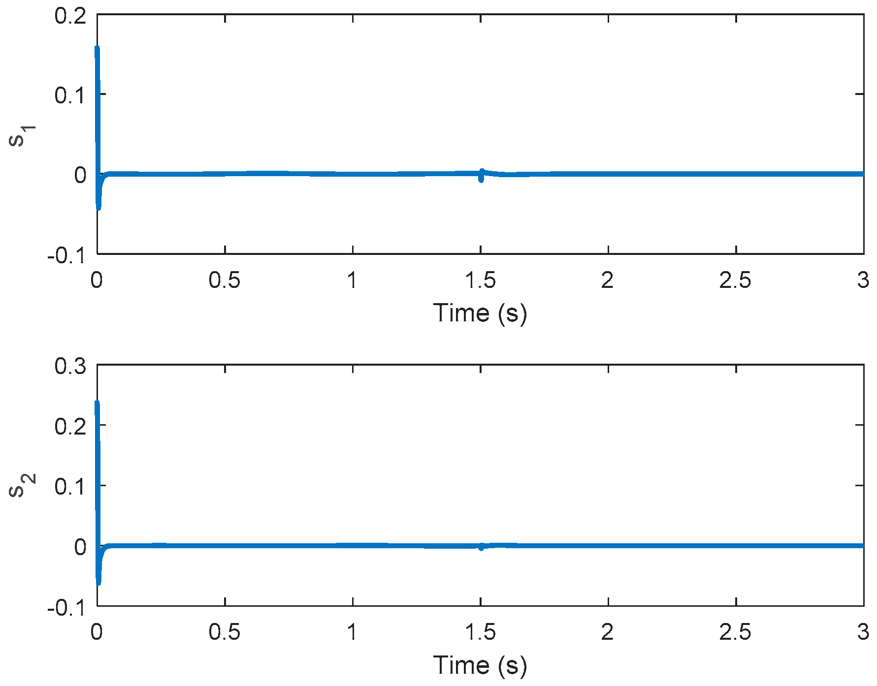
We give a sliding surface as
s ( t ) = C s η ( t ) 0 t ( C s A ¯ p i d η ( t ) K η ( t ) + u ¯ ( t ) ) d t ,
where
C s = [ B p i d 0 ] ,
the equivalent control u e q ( t ) in the sliding manifold ( s ˙ ( t ) = 0 ) is obtained by
u e q ( t ) = K η ( t ) + u ¯ ( t ) d g ( x , t ) .
We lack of the information of perturbation d g ( x , t ) ; hence, the underdetermined estimation of d g ( x , t ) named by d ^ g ( t ) will be design first, then the PI-type controller gain K and control law u ¯ ( t ) will be discussed in detail later, respectively.
Lemma 1. 
In the works [15,21], the authors indicate that the perturbation is assumed to be slowly time-varying; therefore, the derivative of perturbation equal is (near) to zero. Generally, it is reasonable to suppose that
d ˙ g ( x , t ) = 0 ,
when the perturbation is slowly time-varying and changes slightly relative to the observer dynamics with high gain property.
Give the perturbation estimator as
d ^ g ( t ) = k o ( s ( t ) + ( γ s ( t ) + σ s a t ( s ( t ) ) ) d t ) ,
where k o is the positive parameter for the perturbation estimator. In the control law (15), the nonlinear perturbation d g ( x , t ) is unknown so that the control law cannot be achieved. Therefore, the perturbation estimator (17) can be utilized to replace the unknown nonlinear perturbation d g ( x , t ) . Now, the SMC controller u ± ( t ) and SMC-based control law can be designed by
u ± ( t ) = γ s ( t ) σ s a t ( s ( t ) ) ,
u ( t ) = K η ( t ) d ^ g ( t ) + u ± ( t ) + u ¯ ( t ) ,
where γ and σ denote arbitrary nonnegative value so that the trajectories of SMC converge to the sliding manifold and the unknown nonlinear perturbation is estimated consequently.
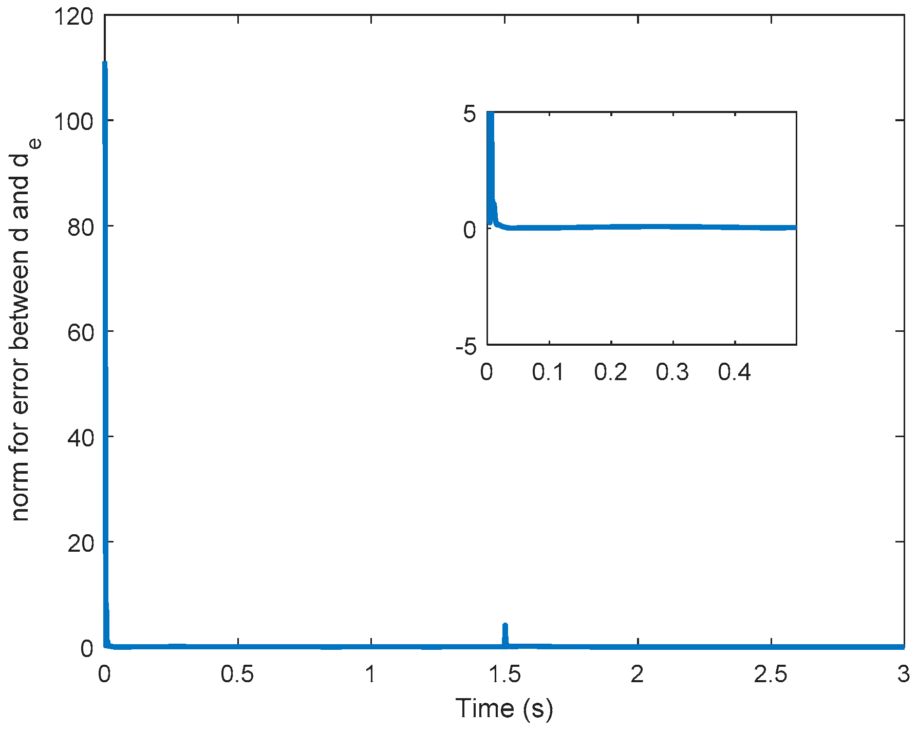
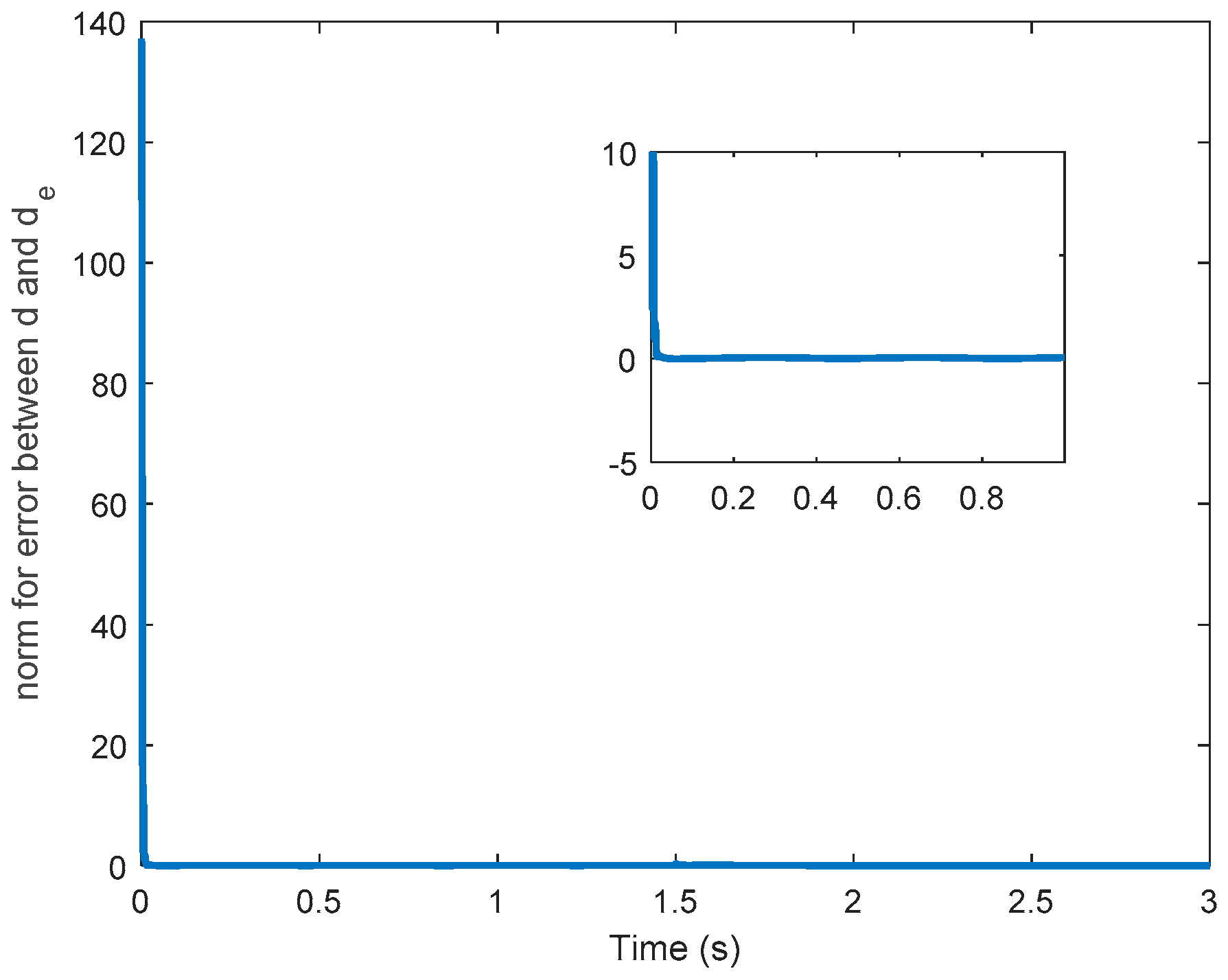
Theorem 1. 
The estimation in (17) leads to the error between the external perturbation and the estimated perturbation converge to zero closely, which implies
d ˜ g ( t ) = d g ( x , t ) d ^ g ( t ) 0 .
Proof. 
See Appendix A. □
Remark 2. 
To avoid the undesired chattering phenomenon in the SMC, the sign function can be replaced by a smooth and continuous saturation function [41].
s a t ( s ( t ) ) = [ s 1 ( t ) | s 1 ( t ) | + δ 1 s i ( t ) | s i ( t ) | + δ i ] T ,
where δ i is an arbitrary small positive constant. If δ i equals to zero, the saturation function s a t ( s ( t ) ) is equivalent to the sign function s i g n ( s ( t ) ) . While the controlled system with direct feed-though term, the undesired chattering phenomenon affects the controlled system output directly. Hence, the saturation function should be smooth enough; in other words, the parameter δ i should be selected properly. Therefore, the undesired chattering phenomenon can be avoided, especially if the controlled system has direct feed-though term.
According to Theorem 1, the sliding manifold is reached and substituting (19) and (20) into (11) and (12), one has
η ˙ ( t ) = A ¯ p i d c η ( t ) + B ¯ p i d 1 u ¯ ( t ) B ¯ p i d 3 d ^ g ( t ) r p i d ( t ) ,
y ( t ) = C ¯ p i d c η ( t ) + D ¯ p i d 1 u ¯ ( t ) D d ^ g ( t ) ,
where A ¯ p i d c = A ¯ p i d B ¯ p i d 1 K , C ¯ p i d c = C ¯ p i d D ¯ p i d 1 K , B ¯ p i d 3 = [ 0 n × m D ] and d ˜ g ( t ) = d g ( x , t ) d ^ g ( t ) .
Lemma 2. 
[16] Let ( A ¯ p i d ,   B ¯ p i d 1 ) be the pair of the given open-loop system and h 0 represent the prescribed degree of relative stability. The eigenvalues of the closed-loop system A ¯ p i d B ¯ p i d 1 ( R 1 B ¯ p i d 1 T P ) lie on the left of the h vertical line with the matrix P being the solution of the Riccati equation
( A ¯ p i d + h I n ) T P + P ( A ¯ p i d + h I n ) P B ¯ p i d 1 R 1 B ¯ p i d 1 T P + Q = 0 ,
where the matrix I n is an identity matrix.
In order to track the reference trajectory, the linear quadratic method is applied to the tracker design. The PI controller gain K can be described as
K = [ K P K I ] = R c 1 ( B ¯ p i d 1 T P + N T ) ,
where R c = R + D ¯ p i d 1 T Q D ¯ p i d 1 , N = C ¯ p i d T Q D ¯ p i d 1 , K P m × n , and K I m × p . To design the controller gain K consisting of K P and K I , we temporarily do not take the perturbation estimator d ^ g ( x , t ) and the control law u ¯ ( t ) into consideration in (22) and (23). Both the d ^ g ( x , t ) and u ¯ ( t ) will be discussed based on the final-value theorem in detail.
Let the quadratic performance index for the output tracking problem be defined as
J = 1 2 0 t f { [ y ( τ ) r ( τ ) ] T Q [ y ( τ ) r ( τ ) ] + u * T ( τ ) R u * ( τ ) } d τ ,
where t f denotes the final time, as well as Q = 10 q I p p × p with q 0 and R = I m m × m are the appropriate weighting matrices. Consider the performance index in (25), to calculate the lower value for the controlled system output y ( t ) ; hence, we obtain r ( t ) = 0   ( r ( τ ) = 0 ) first, then utilize the final-value theorem to minimize the performance index [11]. Thus, consider Lemma 2 and (25), the algebraic Riccati equation is given by
( A ¯ p i d + h I n ) T P + P ( A ¯ p i d + h I n ) ( B ¯ p i d 1 T P + N T ) T R 1 ( B ¯ p i d 1 T P + N T ) + C ¯ p i d T Q C ¯ p i d = 0 .
Solving the matrix P from the algebraic Riccati equation then the control gain K can be constructed. Notice that the PI gains in K are determined based on the linear model ( A ¯ p i d ,   B ¯ p i d 1 ,   C ¯ p i d ,   D ¯ p i d 1 ) first, then take the perturbation estimator d ^ g ( t ) into consideration to determine the control law u ¯ ( t ) in (22) and (23), based on the final-value theorem which will be discussed in detail later.
Finally, it is desirable to determine the u ¯ ( t ) term in (19). Since Lemma 2 is utilized, then the traditional LQAT cannot be adopted to design the control law u ¯ ( t ) . Therefore, the final-value theorem can be utilized to find out the control law u ¯ ( t ) . Since, the PI controller gain K has been chosen, the sliding mode is reached and d ˜ ( t ) is convergence then the control law u ¯ ( t ) can be calculated by the final-value theorem.
Theorem 2. 
The u ¯ ( t ) term is determined based on the integration-term-free augmented system in (22) and (23), where u ¯ ( t ) = [ C p i d c ( A p i d c ) 1 B + D p i d 1 ] { r ( t ) + D d ^ g ( t ) } .
Proof. 
See Appendix B. □
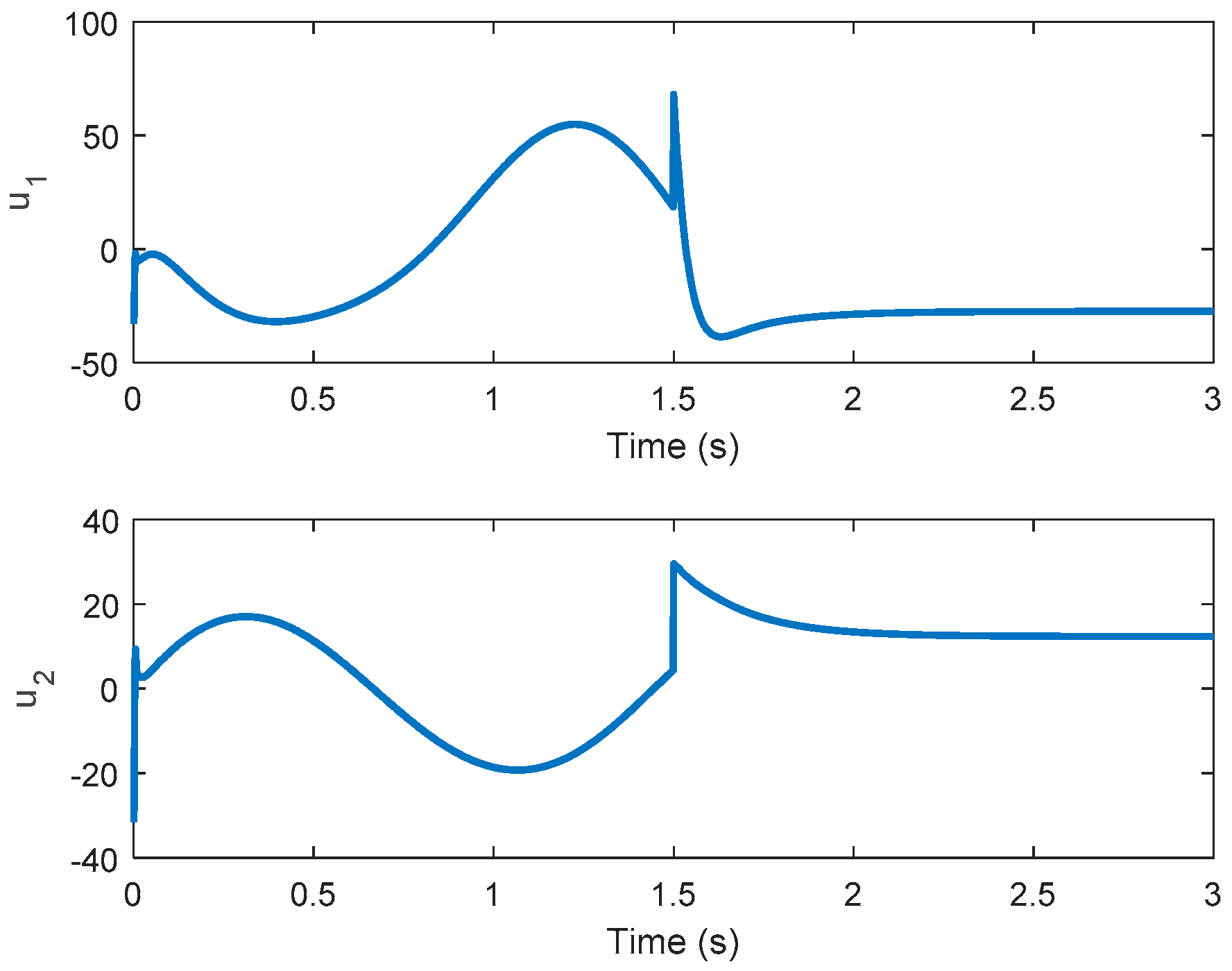
Finally, based on Theorem 2, the desire control law can be described as
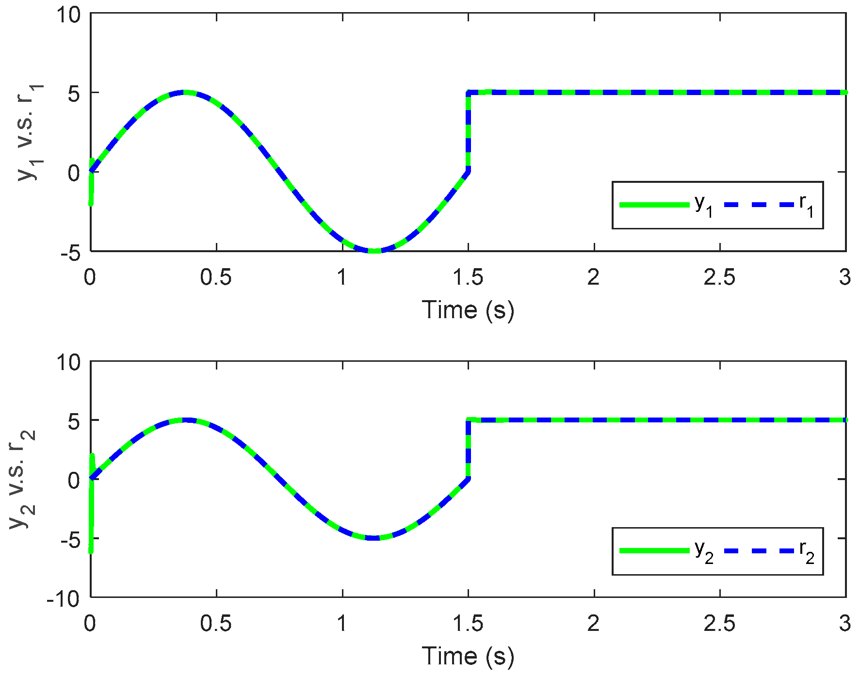
u ( t ) = K η ( t ) d ^ g ( t ) + u ± ( t ) + u ¯ ( t ) + K D x ˙   .
Remark 3. 
If the α equals to 1, the PID-type controller reduces to the PI-type controller. The control law in (27) is utilized to minimize the tracking performance in (25). Therefore, the controlled system output y ( t ) can track the reference trajectory r ( t ) and the tracking error can be minimized.

3. Introduction of DNA Algorithm and Taguchi Method

3.1. DNA Algorithm

The following statements demonstrate the detailed information of DNA algorithm [31,32] operators.
A. Definition of cost function: This step defines a cost function to calculate the cost value of each individual, retain excellent chromosomes, and eliminate adverse chromosomes.
B. Reproduction: Similar to cell division, reproduction is focused on survival of the fittest. Hence, the worse chromosomes will decrease in every generation. Roulette wheel selection is one common technique to implement the proportional selection. Another way to reproduce the better population is the tournament selection. Compared with the roulette wheel selection, the tournament selection only requires the better cost values of the chromosome.
C. Crossover: After reproduction, the chromosomes mate with each other to execute the crossover operator. Crossover exchanges information between two individuals and generates two offspring. The crossover probability p c can be decided to our demand where p c > 0 .
D. Mutation: In natural biological system, creatures mutate by themselves in order to adapt to the external environment. Each chromosome undergoes mutation with a fixed probability p m where p m > 0 . Generally, p m is set to be much lower than p c in order to prevent from being unable to converge.
E. Enzyme/Virus: Enzyme and virus operators are similar to mutation operator, but the most different part is to change structure of the chromosome instead of value of the chromosome. Enzyme operator loses part of segments in chromosome; on the other hand, the virus operator increases an additional part of chromosome. Each chromosome undergoes enzyme and virus with positive probabilities p e and p v , respectively.
F. Termination criteria: This step provides two methods to establish a termination criterion. One is the pre-specified iteration number. Another one is reaching the tolerable error representing the algorithm that converges to the optimal solution or approaching optimal solution.

3.2. Taguchi Method

Taguchi method is a powerful and functional tool in optimization for quality [33,34,39,40]. Taguchi method uses less combination of experiments to obtain the useful information and searches the tendency of optimization to prevent from the cause of sensitive variation. The primary tools of the Taguchi method are the orthogonal array and the signal-to-noise ratio (SNR).
A. Orthogonal array: An orthogonal array can use fewer experiments than full factorial experiments. The normal expression of two-level orthogonal arrays is
L N t ( 2 N t 1 ) ,
where N t = 2 k t denotes number of experimental runs, k t denotes a positive integer which is greater than one, 2 denotes number of levels for each factor, and N t 1 denotes number of columns in the orthogonal array.
B. SNR: Two criteria are used to determine SNR, i.e., smaller is better or larger is better. In the case of the smaller is better characteristic, let two sets of data be described by [ z 1   ,   z 2   ,     ,   z n s ] and [ z ¯ 1   ,   z ¯ 2   ,     ,   z ¯ n s ] . The mean squared deviations from the target value of the quality characteristic are described by
S 1 = 1 n s i s = 1 n s z i s 2
and
S 2 = 1 n s i s = 1 n s z ¯ i s 2 .
In order to shift the mean squared deviation to a suitable situation, utilize the transformation and describe the ratio in decibels
S ¯ 1 = 10 log ( 1 n s i s = 1 n s z i s 2 )
and
S ¯ 2 = 10 log ( 1 n s i s = 1 n s z ¯ i s 2 ) .
After calculating, the SNRs will be compared to decide the better level. Therefore, we can determine the better levels for each factor in less experiment. In the case of larger is better characteristic can refer to the literature [34].

4. Hybrid Taguchi and Real Coded DNA Algorithm

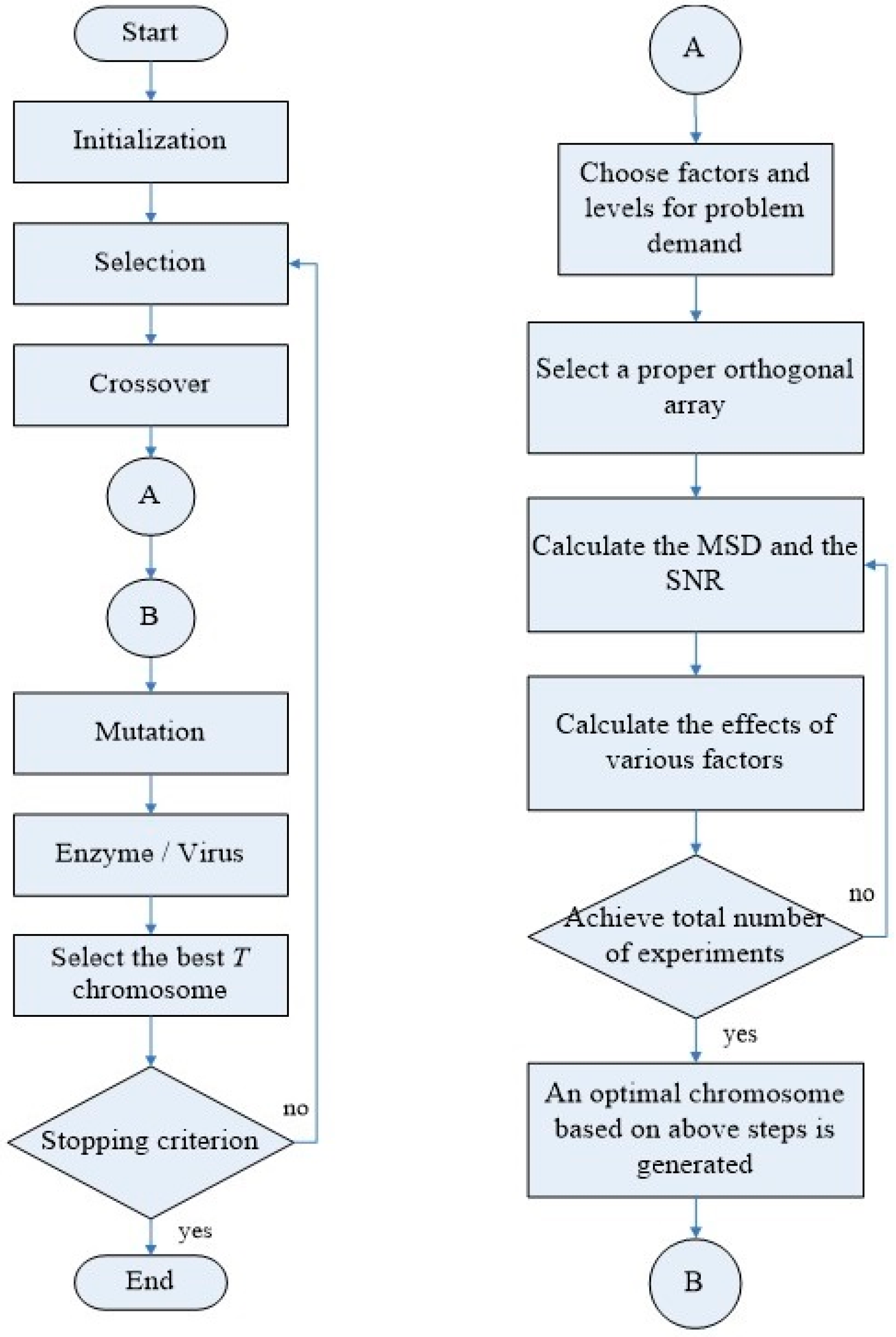
In this section, we are going to take advantage of DNA algorithm and Taguchi method in real coded scheme and combine with the controller design mentioned previously to select a suitable tracking controller. The detailed steps are described in Figure 1 and illustrated in the following statements.
Step 1: Coding strategy: Define a set of chromosomes including the PID gain matrices K P ,   K I ,   K D in the block vector form as follows
C = [ K P K I K D ] .
The previously mentioned controllers can be composed of P controller, PI controller, PD controller, and PID controller. Therefore, definitions of various controller variables are C P i = [ K P i 0 0 ] , C P I i = [ K P i K I i 0 ] , C P D i = [ K P i 0 K D i ] , and C P I D i = [ K P i K I i K D i ] , where i denotes the i   th chromosome in the whole group.
Step 2: Initialization: Before we search a solution to approximate the optimal solution, we need to generate T chromosomes for the population, which is called primitive group. To determine the different gain values in every chromosome, we select the parameters α in [ 0.3 ,   1 ] and q in [ 0 ,   q ¯ ] (for example q ¯ = 2 ) randomly to create four optimal chromosomes for each type controller, and select a gain matrix β I m × m randomly to multiply the optimal chromosomes for other chromosomes until the population is reached. Each component of β I is given a range by [ 0 , 1 ] . Generally, the size of the primitive group depends on the problem complexity; in other words, the more complicated the problem, the larger the primitive group we need. In the experiment, we generate T 4 chromosomes for each type of controller.
Step 3: Reproduction: Tournament selection can be adopted to find the lower cost value for the next population.
Step 4: Crossover: The offspring chromosome has the partial characteristic from the parents after crossover. Refer to [31,34,35], a real coded crossover operator is defined and rewritten as follows
C o f f s p r i n g 1 = β c C p a r e n t 1 + ( 1 β c ) C p a r e n t 2 ,
where C p a r e n t 1 and C p a r e n t 2 represent different chromosomes. The parameter β c is randomly selected and defined in a range [ 0 , 1 ] . The crossover operator is allowed to mate with identical type controllers in the mating pool. For instance, a PI-type controller parameter C P I i only mates with the same feature chromosome.
Step 5: Choosing a proper orthogonal array: Determine the number of factors and levels to construct a suitable orthogonal array L 4 ( 2 3 ) for the problem demand. In the simulation, we choose three factors to make an experiment and the factors are the PID parameters. A two-level orthogonal array is studied.
Step 6: Selecting chromosomes and Taguchi experiments: This step can do ρ runs to generate ρ better chromosomes into every generation. Select a best chromosome and randomly choose another chromosome from the population. Both chromosomes are obtained to execute Taguchi method and find the better solution. In each generation, both chromosomes can be the same type of controllers or different type controllers. For example, both chromosomes C 1 ( P 1 , I 1 , D 1 ) and C 2 ( P 2 , I 2 , D 2 ) are the levels to be selected and each PID parameter is the factor in the orthogonal array. In this paper, the orthogonal array selects L 4 ( 2 3 ) . The P 1 , I 1 and D 1 are represented level 1 and the P 2 , I 2 and D 2 are represented level 2. Calculate the SNR of each experiment in the orthogonal array, then calculate the effect of the various factors. The tracking performance is obtained and the small one is best. The formulation of SNR can be rewritten as ρ κ j = 1 2 i s = 1 2 J c j i s where κ represents the number of factor, j represents the number of level ( J c to be defined later), and the smaller one can be obtained. After the orthogonal array experiment, the smaller SNRs are obtained to find the best factors and the best chromosome can be found by each level. For example, level 1 is obtained in the factor P such that P 1 is selected; level 2 is obtained in the factor I , such that I 2 can be selected; level 1 is obtained in the factor D such that D 1 is selected. Based on the above description, the best chromosome is C B T ( P 1 , I 2 , D 1 ) .
Step 7: Mutation: Real coded changes its value by extending or shortening the scalar. Refer to [31,34,35], we can re-implement the mutation operator as the following
C o f f s p r i n g 2 = C p a r e n t + 2 β m C p a r e n t ,
where β m is randomly selected in a range [ 1   ,   1 ] . By doing this way, it changes both the scalar and the direction to achieve mutation operator.
Step 8: Enzyme/Virus: Select two chromosomes from the population. Enzyme and virus operators can provide us with a suitable controller type. Two different type chromosomes from the pool of {P, PI, PD, PID} are randomly selected. For instance, the former operator can transform PID controller to P controller, PI controller or PD controller; the latter operator transforms P controller to PI controller, PD controller, or PID controller.
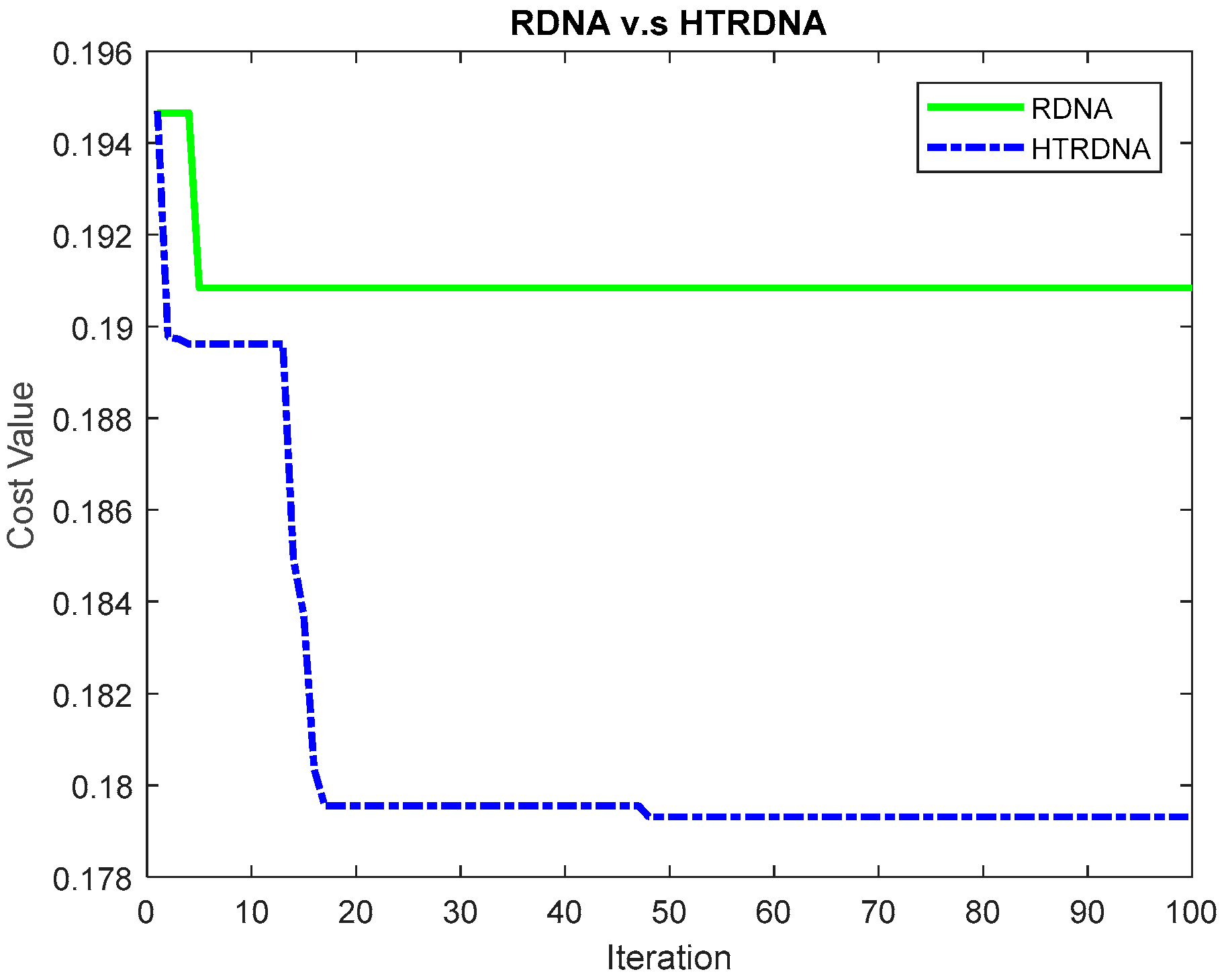
Step 9: Calculating cost value: In order to evolve the population, the cost function is employed to evaluate the value of each chromosome and the minimum one is the best chromosome. We define the cost function as
J c = 0 t f { w 1 ( j 1 = 1 p | e y j 1 ( τ ) | ) + w 2 ( j 2 = 1 m | u j 2 ( τ ) | ) } d τ ,
where e y ( τ ) = [ e y 1 ( τ ) , e y 2 ( τ ) , , e y p ( τ ) ] T denotes the error between the output and the pre-specified trajectory, u ( τ ) = [ u 1 ( τ ) , u 2 ( τ ) , , u m ( τ ) ] T denotes the control force, and J c denotes the cost value.
Step 10: Stopping criterion: If the stopping criterion is reached, then the algorithm is terminated. Otherwise, return to Step 3 and continue to Step 10.

5. Illustrative Examples

In this section, two numerical simulations are given to illustrate the proposed fixed (optimal-based robust tracker) and flexible (HTRDNA-based robust tracker) trackers, respectively.

5.1. Fixed PID-Type Controller

To verify effectiveness of the proposed PID-based robust tracker, the following example is considered. Consider the nonlinear, Chen’s chaotic system described as
{ x ˙ 1 ( t ) = a ( x 2 ( t ) x 1 ( t ) ) x ˙ 2 ( t ) = ( c a ) x 1 ( t ) x 1 ( t ) x 3 ( t ) + c x 2 ( t ) + u 1 ( t ) + d 1 ( x , t ) x ˙ 3 ( t ) = x 1 ( t ) x 2 ( t ) b x 3 ( t ) + u 2 ( t ) + d 2 ( x , t ) ,
or in the general form
x ˙ ( t ) = A x ( t ) + B ( u ( t ) + g ( x , t ) + d ( x , t ) ) ,
where A = [ a a 0 c a c 0 0 0 b ] , B = [ 0 0 1 0 0 1 ] , x ( t ) = [ x 1 ( t ) x 2 ( t ) x 3 ( t ) ] , u * ( t ) = [ u 1 * ( t ) u 2 * ( t ) ] , g ( x , t ) = [ x 1 ( t ) x 3 ( t ) x 1 ( t ) x 2 ( t ) ] , d ( x , t ) = [ d 1 ( x , t ) d 2 ( x , t ) ] , in which a = 35 , b = 3 , c = 28 , x 3 , u ( t ) 2 and the initial condition is selected as x ( 0 ) = [ 0.5 0.2 0.3 ] T . The bounded nonlinear perturbation and the reference trajectory r ( t ) are, respectively, given by
d g ( x , t ) = [ cos ( x 1 ) 0 0 sin ( x 2 ) ] [ 0.3 0 0 0 0.4 0.1 ] x ( t ) + g ( x , t )
and
r ( t ) = { [ 5 sin ( 2 π t / 1.5 ) 5 sin ( 2 π t / 1.5 ) ] T , t 1.5 sec [ 5 5 ] T , t > 1.5 sec .
Let the output be represented by the general form
y ( t ) = C x ( t ) + D u ( t ) ,
where C = [ 0.5 5 0 0 0 0.5 ] ,   D = [ 0.1 0 0 0.2 ] , y ( t ) = [ y 1 ( t ) y 2 ( t ) ] , in which y 2 .
We set the matrix pair { Q ,   R } = { 10 3 I 2 ,   I 2 } for the controller design, k o = 350 , h = 5 and α = 0.8 to yield K D = [ 0 0.2 0 0 0 0.2 ] , M = I 3 B K D = [ 1 0 0 0 0.8 0 0 0 0.8 ] , A ¯ p i d = [ 35 35 0 0 0 8.75 35 0 0 0 0 0 3.75 0 0 0.675 5.7 0 0 0 0 0 0.35 0 0 ] ,   B ¯ p i d = [ 0 0 1.25 0 0 1.25 0.125 0 0 0.25 ] ,   C ¯ p i d = [ 0.675 5.70 0 0 0 0 0 0.35 0 0 ] , D p i d 1 = [ 0.125 0 0 0.25 ] , D p i d 2 = [ 0.025 0 0 0.05 ] , C s = [ 0 0.8 0 0 0 0 0 0.8 0 0 ] , γ = 100 , σ = 0.1 and δ = 10 3 . The PI gain matrices can be obtained as below
K = [ K P K I ] = [ 5.503 46.1477 0 82.7264 0 0 0 1.3867 0 40.1473 ] ,
where K P 2 × 3 and K I 2 × 2 . The sliding surface and fixed PID-type controller are given in (13) and (27), respectively.
Figure 2, Figure 3 and Figure 4 demonstrate the tracking performance between the controlled system output y ( t ) and the pre-specify trajectory r ( t ) . The sliding surface is shown in Figure 5. The estimation error between perturbation estimator and perturbation is shown in Figure 6. Figure 2, Figure 3, Figure 4, Figure 5 and Figure 6 demonstrate a satisfied performance based on the proposed robust tracker for the system with unknown perturbation.

5.2. Flexible PID-Type Controller Based on the HTRDNA

To improve the tracking performance of the proposed PID-based robust tracker, the proposed HTRDNA is adopted. Consider the same Chen’s chaotic system given in Section 5.1. For searching the best cost value during the iterative process, we define the cost function as
J c = 0 t f { w 1 ( j 1 = 1 p | e y j 1 ( τ ) | ) + w 2 ( j 2 = 1 m | u j 2 ( τ ) | ) } d τ ,
where e y ( τ ) = [ e y 1 ( τ ) , e y 2 ( τ ) , , e y p ( τ ) ] T denotes the error between the output and the pre-specified trajectory, u ( τ ) = [ u 1 ( τ ) , u 2 ( τ ) , , u m ( τ ) ] T denotes the control force, J c denotes the cost value.
Here, we hope to apply the HTRDNA algorithm to seek for the best one from four kinds of PID-type controllers. The parameters are chosen as follows: The maximum iteration number is 100, probability of crossover p c = 0.5 , probability of mutation p m = 0.01 , probability of enzyme p e = 0.01 , probability of virus p v = 0.01 , the orthogonal array select L 4 ( 2 3 ) , the weighting w 1 = 1 and w 2 = 10 3 . The resultant controller selected based on the HTRDNA algorithm is the PID-type controller and its parameters are K P = [ 5.0668 49.8911 0 0 0 2.4501 ] ,   K I = [ 102.4782 0.0001 0.0002 50.7663 ]   and   K D = [ 0 0.0081 0.0061 0 0.0019 0.0096 ] . The sliding surface and fixed PID-type controller are given in (13) and (27), respectively.
Figure 7, Figure 8, Figure 9, Figure 10 and Figure 11 demonstrate a quite satisfied tracking performance based on the proposed method. According to Figure 3 and Figure 8, the proposed HTRDNA algorithm can improve the error performance by considering the performance index in (40). Figure 4 and Figure 9 show the control input without undesired chartering phenomenon by using the proposed control law (27). Compare Figure 4 with Figure 9, Figure 9 shows that the control input is constrained by the performance index in (40). Figure 6 and Figure 11 show that the error of perturbation estimation is converged. The simulation results demonstrate the validity of the proposed perturbation estimator method. Furthermore, based on the cost function (40), Figure 12 shows that the proposed flexible PID-type controller outperforms the fixed PID-type controller. In addition, Figure 12 shows that the proposed HTRDNA algorithm outperforms the real code DNA (RDNA) algorithm. Consider the performance index (40) to Section 5.1, the cost value is 0.2129. After HTRDNA algorithm optimization, the cost value is 0.1793. Compare Section 5.1 with Section 5.2, the proposed HTRDNA algorithm can optimize the controller and improve the tracking performance. Based on the above description, the newly proposed HTRDNA algorithm can improve the performance for the proposed controller.

6. Conclusions

A robust tracker design for a class of nonlinear controlled systems with/without direct feed-through term and unknown nonlinear perturbation is proposed in this paper. Based on LQAT, by taking linear transformation and augmented state, a simple approach for the PID-type controller with SMC and perturbation estimator is proposed. The designed perturbation estimator is employed to eliminate the unknown nonlinear perturbation so that the better performance can be achieved. To improve the efficiency of real coded DNA algorithm, this paper utilizes the advantage of the Taguchi method to real coded DNA algorithm so that the HTRDNA algorithm is newly proposed for the PID controller optimization. Due to the SMC with fast response, SMC is employed to cope with the nonlinear perturbation and then HTRDNA algorithm can be utilized to tune the PID controller type and its parameters. Simulation results demonstrate the validity of our proposed method.

Author Contributions

All authors contributed to the paper. J.-S.F. wrote the manuscript with the supervision from J.-J.Y. and J.S.-H.T. C.-H.T. and S.-M.G. are responsible for the simulation of the proposed robust tracker.

Funding

This work was financially supported by the Ministry of Science and Technology, Taiwan, under MOST-107-2221-E-167 -032 -MY2.

Conflicts of Interest

The authors declare no conflict of interest.

Appendix A

Proof of Theorem A1. 
Substitute (19) and (20) into the derivative of sliding surface in (13) to obtain
s ˙ ( t ) = d ˜ g ( t ) γ s ( t ) .
Differentiating (17), one has
d ^ ˙ ( t ) = k o ( s ˙ ( t ) + γ s ( t ) ) = k o ( d ˜ g ( t ) γ s ( t ) + γ s ( t ) ) = k o d ˜ g ( t ) .
Substituting (16) and (A2) into the differentiation of (20) yields
d ˜ ˙ g ( t ) = d ˙ g ( x , t ) d ^ ˙ g ( t ) = d ˙ g ( x , t ) k o d ˜ g ( t ) = k o d ˜ g ( t ) .
If the gain k o is selected to be a positive value, the error of (20) can converge and approximate to zero. In other words, the estimated perturbation can approximate to the unknown perturbation at the steady state.
Consider a candidate Lyapunov function as
v ( s ) = 1 2 s T s ,
and taking the derivative of v ( s ) in (A4) gives
v ˙ ( s ) = s T s ˙ = s T ( d ˜ g ( x , t ) γ s σ s a t ( s ( t ) ) ) d ˜ g ( x , t ) s γ s 2 σ s γ s 2 σ s .
Equations (A3)–(A5) show that the sliding mode states can reach the defined sliding manifold in finite time with the given parameters γ > 0 and σ > 0 ; therefore, (17) can estimate the unknown external perturbation and eliminate its impact directly. In addition, when d ˜ g ( t ) equals or closes to zero, the controller in (19) can achieve a desired tracking performance. □

Appendix B

Proof of Theorem A2. 
Consider a linear time-invariant system with the PI-type controller and underdetermined u ¯ ( t ) term described by
x ˙ ( t ) = A x ( t ) + B ( u ¯ ( t ) K P x ( t ) K I e y ( t ) d t ) ,
y ( t ) = C x ( t ) + D ( u ¯ ( t ) K P x ( t ) K I e y ( t ) d t ) .
Take the Laplace transform of the tracking error to obtain the following equations
E y ( s ) = Y ( s ) R s = { ( C D K P ) [ s I n ( A B K P ) ] 1 B + D } ( U ¯ s s K I E ( s ) s ) R s s ,
where U ¯ s and R s are the steady-state values of u ¯ ( t ) and r ( t ) , respectively, during any time period, if u ¯ ( t ) and r ( t ) change slightly relative to the high gain property controlled system dynamics. Using the final-value theorem to (A8), one has
lim s 0 s E y ( s ) = lim s 0 s [ W ( U ¯ s s K i E ( s ) s ) R s s ] = lim s 0 [ W ( U ¯ ( s ) K i E ( s ) ) R s ] ,
where
W = ( C D K P ) [ s I n ( A B K P ) ] 1 B + D .
Rearrange (A9) to have
lim s 0 ( s I n + K I W ) E y ( s ) = lim s 0 ( W U ¯ s R s ) ,
which implies
lim s 0 { ( C D K P ) [ s I n ( A B K P ) ] 1 B + D } U ¯ s R s = 0
for lim s 0 s E y ( s ) = 0 . From (A10), we can infer that it is sufficient to derive the controller u ¯ ( t ) in (22) and (23) by applying the final-value theorem without the integral term.
According to Theorem 1 and Theorem 2, SMC is reached and the perturbation is estimated by the perturbation estimator. Then, take Laplace transforms of (22) and (23) without integral term to obtain
Y ( s ) = C p i d c ( s I n A p i d c ) 1 B p i d U ¯ s s + D p i d 1 ( U ¯ s s D ^ g s s ) = [ C p i d c ( s I n A p i d c ) 1 B p i d + D p i d 1 ] U ¯ s s D D ^ g s s ,
where D ^ g s is the steady-state values of d ^ g ( t ) , during any time period, if d ^ g ( t ) changes slightly relative to the high gain property controlled system dynamics. Applying the final-value theorem to the tracking error and forcing it to be zero yields
lim s 0 s E y ( s ) = lim s 0 s ( Y ( s ) R s )   = [ C p i d c ( A p i d c ) 1 B p i d + D p i d 1 ] U ¯ s D D ^ g s R s = 0 ,
so that in general, one has
u ¯ ( t ) = [ C p i d c ( A p i d c ) 1 B + D p i d 1 ] { r ( t ) + D d ^ g ( t ) } ,
where
A p i d c = A p i d B p i d K P , C p i d c = C p i d D p i d 1 K P .
 □

References

  1. Ang, K.; Chong, G.; Li, Y. PID control system analysis, design, and technology. IEEE Trans. Control Syst. Technol. 2005, 13, 559–576. [Google Scholar]
  2. Åström, K.J.; Hägglund, T. PID Controllers: Theory, Design, and Tuning; ISA, The Instrumentation, Systems, and Automation Society: Pittsburgh, PA, USA, 1995. [Google Scholar]
  3. Gaing, Z.L. A particle swarm optimization approach for optimum design of PID controller in AVR system. IEEE Trans. Energy Convers. 2004, 19, 384–391. [Google Scholar] [CrossRef]
  4. Nazaruddin, Y.Y.; Andrini, A.D.; Anditio, B. PSO Based PID Controller for Quadrotor with Virtual Sensor. IFAC-PapersOnLine 2018, 51, 358–363. [Google Scholar] [CrossRef]
  5. Abdelaziz, T.H.S.; Valasek, M. Pole-placement for SISO Linear Systems by State-derivative Feedback. IEE Proc. Control Theory Appl. 2004, 151, 377–385. [Google Scholar] [CrossRef]
  6. Cardim, R.; Teixeira, M.C.M.; Assuncao, E.; Covacic, M.R. Design of state-derivative feedback controllers using a state feedback control design. IFAC Proc. Vol. 2007, 40, 22–27. [Google Scholar] [CrossRef]
  7. Zheng, F.; Wang, Q.G.; Lee, T.H. On the design of multivariable PID controllers via LMI approach. Automaticca 2002, 38, 517–526. [Google Scholar] [CrossRef]
  8. Rosinová, D.; Veselý, V. Robust pid decentralized controller design using lmi. IFAC Proc. Vol. 2006, 39, 53–58. [Google Scholar] [CrossRef]
  9. Wang, J.; Zhang, Q.; Xiao, D. PD feedback H control for uncertain singular neutral systems. Adv. Differ. Equ. 2016, 2016, 29. [Google Scholar] [CrossRef]
  10. Shariati, A.; Taghirad, H.D.; Fatehi, A. A neutral system approach to H PD/PI controller design of processes with uncertain input delay. J. Process Control 2014, 24, 144–157. [Google Scholar] [CrossRef]
  11. Singla, M.; Shieh, L.S.; Song, G.; Xie, L.; Zhang, Y. A new optimal sliding mode controller design using scalar sign function. ISA Trans. 2014, 53, 267–279. [Google Scholar] [CrossRef]
  12. Madsen, J.M.; Shieh, L.S.; Guo, S.M. State-Space Digital PID Controller Design for Multivariable Analog Systems with Multiple Time Delays. Asian J. Control 2006, 8, 161–173. [Google Scholar] [CrossRef]
  13. Ebrahimzadeh, F.; Tsai, J.S.H.; Liao, Y.T.; Chung, M.C.; Guo, S.M.; Shieh, L.S.; Wang, L. A generalised optimal linear quadratic tracker with universal applications—Part 1: Continuous-time systems. Int. J. Syst. Sci. 2017, 48, 376–396. [Google Scholar] [CrossRef]
  14. Tsai, J.S.H.; Wang, H.H.; Guo, S.M.; Shieh, L.S.; Canelon, J.I. A case study on the universal compensation improvement mechanism: A robust PID filter-shaped optimal PI tracker for systems with/without disturbances. J. Frankl. Inst. 2018, 355, 3583–3618. [Google Scholar] [CrossRef]
  15. Chen, W.H.; Ballance, D.J.; Gawthrop, P.J.; O’Reilly, J. A nonlinear disturbance observer for robotic manipulators. IEEE Trans. Ind. Electron. 2000, 47, 932–938. [Google Scholar] [CrossRef]
  16. Shieh, S.L.; Dib, M.H.; Sekar, G. Continuous-time quadratic regulators and pseudo-continuous-time quadratic regulators with pole placement in a specific region. IEE Proc. D-Control Theory Appl. 1987, 134, 338–346. [Google Scholar] [CrossRef]
  17. Chang, W.D.; Yan, J.J. Adaptive robust PID controller design based on a sliding mode for uncertain chaotic systems. Chaos Solitons Fractals 2005, 26, 167–175. [Google Scholar] [CrossRef]
  18. Fnaiech, M.A.; Betin, F.; Capolino, G.A.; Fnaiech, F. Fuzzy logic and sliding-mode controls applied to six-phase induction machine with open phases. IEEE Trans. Ind. Electron. 2010, 57, 354–364. [Google Scholar] [CrossRef]
  19. Mondal, S.; Mahanta, C. Chattering free adaptive multivariable sliding mode controller for systems with matched and mismatched uncertainty. ISA Trans. 2013, 52, 335–341. [Google Scholar] [CrossRef]
  20. Singh, Y.; Santhakumar, M. Inverse dynamics and robust sliding mode control of a planar parallel (2-PRP and 1-PPR) robot augmented with a nonlinear disturbance observer. Mech. Mach. Theory 2015, 92, 29–50. [Google Scholar] [CrossRef]
  21. Li, D. Nonlinear disturbance observer-based robust control for spacecraft formation flying. Aerosp. Sci. Technol. 2018, 76, 82–90. [Google Scholar]
  22. Huang, J.; Ri, S.; Fukuda, T.; Wang, Y. A Disturbance Observer based Sliding Mode Control for a Class of Underactuated Robotic System with Mismatched Uncertainties. IEEE Trans. Autom. Control 2019, 64, 2480–2487. [Google Scholar] [CrossRef]
  23. Ahmed, N.; Chen, M. Sliding mode control for quadrotor with disturbance observer. Adv. Mech. Eng. 2018, 10. [Google Scholar] [CrossRef]
  24. Qian, R.; Luo, M.; Zhao, Y.; Zhao, J. Novel Adaptive Sliding Mode Control with Nonlinear Disturbance Observer for SMT Assembly Machine. Math. Probl. Eng. 2016, 2016, 14. [Google Scholar] [CrossRef]
  25. Wang, J.; Li, S.; Yang, J.; Wu, B.; Li, Q. Extended state observer-based sliding mode control for PWM-based DC-DC buck power converter systems with mismatched disturbances. IET Control Theory Appl. 2015, 9, 579–586. [Google Scholar] [CrossRef]
  26. Li, Y.; Zheng, Q.; Yang, L. Design of robust sliding mode control with disturbance observer for multi-axis coordinated traveling system. Comput. Math. Appl. 2012, 64, 759–765. [Google Scholar] [CrossRef]
  27. Hast, M.; Åström, K.J.; Bernhardsson, B.; Boyd, S. PID design by convex-concave optimization. In Proceedings of the 2013 European Control Conference (ECC), Zurich, Switzerland, 17–19 July 2013; pp. 4460–4465. [Google Scholar]
  28. Mercader, P.; Åström, K.J.; Banos, A.; Hägglund, T. Robust PID design based on QFT and convex–concave optimization. IEEE Trans. Control Syst. Technol. 2016, 25, 441–452. [Google Scholar] [CrossRef]
  29. Karimi, A.; Kammer, C. A data-driven approach to robust control of multivariable systems by convex optimization. Automatica 2017, 85, 227–233. [Google Scholar] [CrossRef]
  30. Vijay, M.; Jena, D. PSO based neuro fuzzy sliding mode control for a robot manipulator. J. Electr. Syst. Inf. Technol. 2016, 4, 243–256. [Google Scholar] [CrossRef]
  31. Wu, C.T.; Tien, J.P.; Li, T.H.S. Integration of DNA and real coded GA for the design of PID-like fuzzy controllers. In Proceedings of the 2012 IEEE International Conference on Systems, Man, and Cybernetics (SMC), Seoul, Korea, 14–17 October 2012; pp. 2809–2814. [Google Scholar]
  32. Yourui, H.; Chen, X.; Yihua, H. Optimization for parameter of PID based on DNA genetic algorithm. In Proceedings of the 2005 International Conference on Neural Networks and Brain, Beijing, China, 13–15 October 2005; pp. 859–861. [Google Scholar]
  33. Chou, J.H.; Chen, S.H.; Li, J.J. Application of the Taguchi-genetic method to design an optimal grey-fuzzy controller of a constant turning force system. J. Mater. Process. Technol. 2000, 105, 333–343. [Google Scholar] [CrossRef]
  34. Tsai, J.T.; Liu, T.K.; Chou, J.H. Hybrid Taguchi-genetic algorithm for global numerical optimization. IEEE Trans. Evol. Comput. 2004, 8, 365–377. [Google Scholar] [CrossRef]
  35. Chen, J.L.; Chang, W.D. Feedback linearization control of a two-link robot using a multi-crossover genetic algorithm. Expert Syst. Appl. 2009, 36, 4154–4159. [Google Scholar] [CrossRef]
  36. Zhou, X.; Gao, H.; Zhao, B.; Zhao, L. A GA-based parameters tuning method for an ADRC controller of ISP for aerial remote sensing applications. ISA Trans. 2018, 81, 318–328. [Google Scholar] [CrossRef]
  37. Feng, H.; Yin, C.B.; Weng, W.W.; Ma, W.; Zhou, J.J.; Jia, W.H.; Zhang, Z.L. Robotic excavator trajectory control using an improved GA based PID controller. Mech. Syst. Signal Process 2018, 105, 153–168. [Google Scholar] [CrossRef]
  38. Zemmit, A.; Messalti, S.; Harrag, A. A new improved DTC of doubly fed induction machine using GA-based PI controller. Ain Shams Eng. J. 2017, 9, 1877–1885. [Google Scholar] [CrossRef]
  39. Phadke, M.S. Quality Engineering Using Robust Design; Prentice Hall PTR: Upper Saddle River, NJ, USA, 1995. [Google Scholar]
  40. Ross, P.J. Taguchi Techniques for Quality Engineering: Loss Function, Orthogonal Experiments; Parameter and Tolerance Design, McGraw Hill: New York, NY, USA, 1988. [Google Scholar]
  41. Lin, J.S.; Huang, C.F.; Liao, T.L.; Yan, J.J. Design and implementation of digital secure communication based on synchronized chaotic systems. Digit. Signal Process. 2010, 20, 229–237. [Google Scholar] [CrossRef]
Figure 1. Flow chart for HTRDNA algorithm.
Mathematics 07 01141 g001
Figure 2. Time responses of the closed-loop system with the fixed PID controller and unknown perturbation.
Mathematics 07 01141 g002
Figure 3. Tracking errors of the closed-loop system with the fixed PID controller and unknown perturbation.
Mathematics 07 01141 g003
Figure 4. Control inputs based on the fixed PID controller and unknown perturbation.
Mathematics 07 01141 g004
Figure 5. Sliding manifolds for the fixed PID controller with unknown perturbation.
Mathematics 07 01141 g005
Figure 6. Error between unknown and estimated perturbations.
Mathematics 07 01141 g006
Figure 7. Time responses of the closed-loop system with the flexible PID controller and unknown perturbation.
Mathematics 07 01141 g007
Figure 8. Tracking errors of the closed-loop system with the flexible PID controller and unknown perturbation.
Mathematics 07 01141 g008
Figure 9. Control inputs based on the flexible PID controller and unknown perturbation.
Mathematics 07 01141 g009
Figure 10. Sliding manifolds for the flexible PID controller with unknown perturbation.
Mathematics 07 01141 g010
Figure 11. Error between unknown and estimated perturbations.
Mathematics 07 01141 g011
Figure 12. Evolution of RDNA and HTRDNA algorithm.
Mathematics 07 01141 g012

