Energy-Based Control and LMI-Based Control for a Quadrotor Transporting a Payload

Abstract

This paper presents the control of a quadrotor with a cable-suspended payload. The proposed control structure is a hierarchical scheme consisting of an energy-based control (EBC) to stabilize the vehicle translational dynamics and to attenuate the payload oscillation, together with a nonlinear state feedback controller based on an linear matrix inequality (LMI) to control the quadrotor rotational dynamics. The payload swing control is based on an energy approach and the passivity properties of the system’s translational dynamics. The main advantage of the proposed EBC strategy is that it does not require excessive computations and complex partial differential equations (PDEs) for implementing the control algorithm. We present a new methodology for using an LMI to synthesize the controller gains for Lipschitz nonlinear systems with larger Lipschitz constants than other classical techniques based on LMIs. This theoretical approach is applied to the quadrotor rotational dynamics. Stability proofs based on the Lyapunov theory for the controller design are presented. The designed control scheme allows for the stabilization of the system in all its states for the three-dimensional case. Numerical simulations demonstrating the effectiveness of the controller are provided.

1. Introduction

In recent years, systems for the transportation of suspended-payload using unmanned aerial vehicles (UAVs) have attracted research interest. Some important applications are described in [1]. Quadrotor vehicles exhibit complex dynamic behavior, and if a cable-suspended payload is added to a quadrotor, it increases the complexity of the system because additional degrees of freedom (DOFs) due to the payload oscillation are introduced. Moreover, if uncontrolled, a cable-suspended payload changes the dynamics of the flying vehicle and it can result in an unstable system.

Recently, some control methodologies have been developed to attenuate the payload swing and to solve the general problem of a quadrotor carrying a cable-suspended payload. For example, a control algorithm based on a backstepping strategy is obtained in [2], that ensures trajectory tracking of the quadrotor regardless of the payload swing. However, attitude control of the UAV is not considered. Additionally, a control design for a two-dimensional quadrotor with a cable-suspended payload that enables tracking of the vehicle rotation, the payload rotation, or the payload position is presented in [3], and it was extended to the three-dimensional case in [4].

In [5], the authors develop a nested saturation controller capable of driving the vehicle to a specified position while simultaneously limiting the payload dynamic effect. For this work, Nicotra et al. considered the design for the two-dimensional case only and the attitude control of the vehicle was not considered. Moreover, a feed-forward control algorithm for reducing or canceling the payload’s oscillation is introduced in [6]. This controller was designed by implementing the input shaping theory. In [7], the authors present a geometric controller to exponentially stabilize the aerial robot position while aligning the links vertically below the vehicle. Similarly, a tracking control law for a UAV with a load attached by a cable represented as successively-attached inflexible links was designed in [8]. A fixed-gain geometric PD control strategy is developed to reach the desired goal for a nominal load. An adaptive control law for an aerial robot carrying a payload attached using a cable was presented in [9]. In [10], an algorithm for parameterizing aerial vehicles transporting a payload employing a complementary constraint is presented. A nonlinear attitude controller is developed in [11] to stabilize the altitude, and the translational dynamics control law is introduced by converting the vehicle velocity and position error into rotation control. Rego and Raffo [12] address trajectory tracking for a two-dimensional aerial robot transporting a payload. A discrete-time mixed $H2/H\infty$ linear control strategy is presented. In [13], an active-model-based linear controller is designed for a UAV transporting a payload. A linear model is obtained considering the vehicle in hover flight mode. In [14], a path tracking controller is developed based on existing Lyapunov-based path tracking control laws for free-flying aerial vehicles, which are further backstepped through the vehicle rotation dynamics.

A passivity-based control technique is used in [15] to control the UAV such that cable-suspended payload swing reduction is achieved for the planar case. Here, the attitude control of the vehicle is not considered. Also, interconnection and damping assignment passivity-based control (IDA-PBC) without total energy-shaping for a UAV transporting a cable-suspended payload for planar maneuvers is developed in [16,17]. Two control laws with total energy-shaping are presented in [18], where the closed-loop inertia matrices are modified. These works compute PDEs for synthesizing the control law. For this reason, the control strategy is only designed within the longitudinal plane. The control design for the three-dimensional case yields complex partial differential equations (PDEs).

In the literature, unmanned aerial vehicles have been controlled using energy-based controllers. In [19], the design of two nonlinear controllers to stabilize an aerial vehicle characterized with quaternions and their axis-angle depiction is studied. Also, [20] introduces a PBC for a vertical take-off and landing (VToL) vehicle. An estimator of unmodelled dynamics and external wrench acting on the UAV and based on the momentum of the system is used to compensate such disturbance effects. Moreover, [21] develops an IDA-PBC methodology that is able to change the apparent vehicle dynamical parameters, while [22] proposes a robust control of underactuated aerial manipulators via IDA-PBC.

On the other hand, some works apply control strategies based on linear matrix inequalities to UAVs. In [23], a method for using LMIs to synthesize controller gains for a UAV system is presented. In [24], a nonlinear state feedback controller based on LMIs, and a technique with pole placement constraint (PDC) is synthesized. The requirements of stability and pole placement in the linear matrix inequality (LMI) region are formulated based on the Lyapunov direct method.

In this work, the control approach is based on a hierarchical scheme considering the well-known time-scale separation between rotational and translational dynamics of the quadrotor. On one hand, the objective of this paper was to design an energy-based control law for the outer-loop (i.e., for the underactuated dynamics of the system). This control law is proposed for the three-dimensional case, and it is based on the translation dynamics, which is able to lead the vehicle to a desired position while simultaneously reducing the payload swing. Compared with similar works that present control laws based on passivity and energy, particularly for underactuated systems, the proposed controller avoids solving complex PDEs to obtain the control law. On the other hand, a feedback controller based on an LMI for the inner loop which is fully actuated is presented. The controller based on an LMI for the rotational dynamics results in a control algorithm with relative simplicity and with an easy analysis to demonstrate its stability.

The contribution of this paper is the synthesis of a new controller for a class of Lipschitz nonlinear systems. An important limitation of the classic results for Lipschitz nonlinear systems is that they perform well only for small values of the Lipschitz constant. In the case when the Lipschitz constant is large, most of the existing controller design approaches fail to contribute a solution to the LMI. This article introduces an algorithm that operates for larger Lipschitz constants compared with classical results in the literature.

This paper is organized as follows. Section 2 describes the dynamical model for a three-dimensional aerial vehicle carrying a payload. Section 3 presents an approach for LMI-based Lipschitz nonlinear systems. This theoretical approach is applied to stabilize the quadrotor rotational dynamics. Section 4 proposes an energy-based control to stabilize the vehicle translational dynamics and to attenuate the payload swing. Section 5 presents numerical simulations and results. Finally, Section 6 gives conclusions and perspectives.

2. Dynamic Model

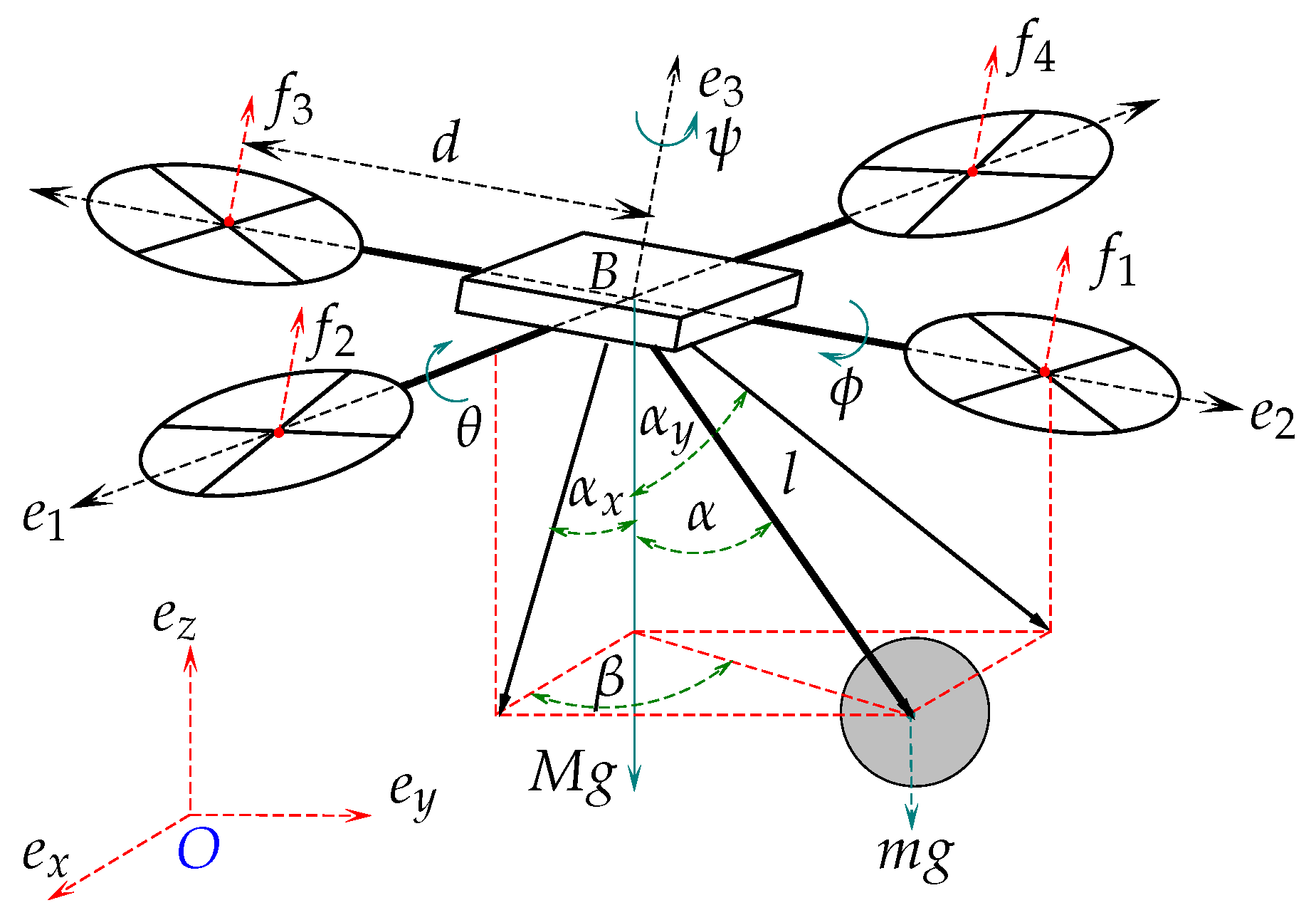
In this section, we present the mathematical model of a quadrotor transporting a payload connected by a cable. The aim is to present a dynamic model that mathematically describes the relationship between the quadrotor, the cable, and the payload. For this purpose, consider a rigid body with mass m, being transported by a quadrotor as shown in Figure 1. Note that in addition to the six DOFs of the UAV, the payload adds another two DOFs, resulting in a system with eight DOFs and four inputs.

The following assumptions were made for modeling the quadrotor with a cable-suspended payload:

(a)

The cable is attached to the center of mass of the quadrotor and the air drag is negligible.

(b)

The cable connecting the payload and the quadrotor fuselage is considered rigid, massless, and inelastic.

(c)

The payload can be considered as a mass point.

(d)

Mass distribution of the quadrotor is symmetrical in the x-y plane.

As shown in Figure 1, the body-fixed frame is defined by $B=\left\{e_1,e_2,e_3\right\}$ and the inertial frame by $O=\left\{e_x,e_y,e_z\right\}$. The location of the mass center of the vehicle relative to O is represented by $\xi ={\left[\begin{array}{ccc}x& y& z\end{array}\right]}^T$, the attitude of the quadrotor is denoted by $\eta ={\left[\begin{array}{ccc}\psi & \theta & \varphi \end{array}\right]}^T$ (i.e., yaw, pitch, and roll, respectively). $\alpha$ defines the payload swing angle in space and has two components ${\alpha }_x$ and ${\alpha }_y$, $\mu ={\left[\begin{array}{cc}{\alpha }_x& {\alpha }_y\end{array}\right]}^T$. ${\alpha }_x$ is the swing angle projected on the $XZ$ plane and ${\alpha }_y$ is the swing angle projected on the $YZ$ plane, $\beta$ represents the angle of the X axis and the projected line of the cable to the Y plane. Thus, the state vector is denoted by $q={\left[\begin{array}{cccccccc}x& y& z& \psi & \theta & \varphi & {\alpha }_x& {\alpha }_y\end{array}\right]}^T\in {\mathbb{R}}^8$. The control input is represented by $u={\left[\begin{array}{cc}f& \tau \end{array}\right]}^T\in {\mathbb{R}}^4$, where $f=f_1+f_2+f_3+f_4$ defines the total thrust magnitude and $\tau ={\left[\begin{array}{ccc}{\tau }_{\psi }& {\tau }_{\theta }& {\tau }_{\varphi }\end{array}\right]}^T$ denotes the input torques.

The mass of the quadrotor and the payload are defined by M and m, respectively. The length of the cable is represented by l, the gravitational acceleration by g. Finally, the distance between the motors and the gravity center is equal to d.

In this work, the system is modeled using the Euler–Lagrange formulation.

2.1. Euler–Lagrange Formulation

Let ${\xi }_p={\left[\begin{array}{ccc}{x}_p& y_p& z_p\end{array}\right]}^T\in {\mathbb{R}}^3$ be the payload position in the inertial frame. Thus, the quadrotor and payload positions are related by

$${\xi }_p=\xi +lp,$$

where

$$p={\left[\begin{array}{ccc}\sin \left({\alpha }_x\right)\cos \left({\alpha }_y\right)& \sin \left({\alpha }_y\right)& -\cos \left({\alpha }_x\right)\cos \left({\alpha }_y\right)\end{array}\right]}^T.$$

The equations of motion are obtained using the Euler–Lagrange method. The kinetic energy of the payload-quadrotor system is given by

$$K_{Q-P}=\frac{1}{2}M{\dot{\xi }}^T\dot{\xi }+\frac{1}{2}m{{\dot{\xi }}_p}^T{\dot{\xi }}_p+\frac{1}{2}{\dot{\eta }}^{T}J\dot{\eta },$$

(1)

where $J=diag{[I_{xx},I_{yy},I_{zz}]}_{3\times 3}$ is a symmetric positive definite constant inertia matrix of the quadrotor with respect to B.

The total potential energy is defined by

$$V_{Q-P}=(M+m)gz-mgl\cos \left({\alpha }_x\right)\cos \left({\alpha }_y\right).$$

(2)

From (1) and (2), the Lagrangian is given by

$$L=\frac{1}{2}M{\dot{\xi }}^T\dot{\xi }+\frac{1}{2}m{{\dot{\xi }}_p}^T{\dot{\xi }}_p+\frac{1}{2}{\dot{\eta }}^{T}J\dot{\eta }-(M+m)gz+mgl\cos \left({\alpha }_x\right)\cos \left({\alpha }_y\right).$$

(3)

Using the Lagrangian and the derived formula for the equations of motion:

$$\mathcal{M}\left(q\right)\ddot{q}+C(q,\dot{q})\dot{q}+G\left(q\right)=\overline{B}u,$$

(4)

where $\mathcal{M}\left(q\right)\in {\mathbb{R}}^{8\times 8}$ denotes the inertia matrix, which is symmetric and positive definite, $C(q,\dot{q})\in {\mathbb{R}}^{8\times 8}$ the Coriolis and centrifugal matrix, $G\left(q\right)\in {\mathbb{R}}^8$ the gravitational vector, and the matrix $\overline{B}\in {\mathbb{R}}^{8\times 4}$ is determined by the manner in which the control $u\in {\mathbb{R}}^4$ is the input of the system. These matrices are defined as

$$\mathcal{M}\left(q\right)=\left[\begin{array}{cccccccc}m+M& 0& 0& 0& 0& 0& ml{c}_{{\alpha }_x}{c}_{{\alpha }_y}& -ml{s}_{{\alpha }_x}{s}_{{\alpha }_y}\\ 0& m+M& 0& 0& 0& 0& 0& ml{c}_{{\alpha }_y}\\ 0& 0& m+M& 0& 0& 0& ml{s}_{{\alpha }_x}{c}_{{\alpha }_y}& ml{c}_{{\alpha }_x}{s}_{{\alpha }_y}\\ 0& 0& 0& I_{xx}& 0& 0& 0& 0\\ 0& 0& 0& 0& I_{yy}& 0& 0& 0\\ 0& 0& 0& 0& 0& I_{zz}& 0& 0\\ ml{c}_{{\alpha }_x}{c}_{{\alpha }_y}& 0& ml{s}_{{\alpha }_x}{c}_{{\alpha }_y}& 0& 0& 0& m{l}^2{c}_{{\alpha }_y}^2& 0\\ -ml{s}_{{\alpha }_x}{s}_{{\alpha }_y}& ml{c}_{{\alpha }_y}& ml{c}_{{\alpha }_x}{s}_{{\alpha }_y}& 0& 0& 0& 0& m{l}^2\end{array}\right]$$

$$\begin{array}{cc}\hfill C\left(q\right)=& \left[\begin{array}{cccccc}0& 0& 0& 0& 0& 0\\ 0& 0& 0& 0& 0& 0\\ 0& 0& 0& 0& 0& 0\\ 0& 0& 0& 0& 0& (I_{yy}-I_{zz})\dot{\theta }\\ 0& 0& 0& 0& 0& J_r{\Omega }_r+(I_{zz}-I_{xx})\dot{\psi }\\ 0& 0& 0& 0& (I_{xx}-I_{yy})\dot{\psi }-J_r{\Omega }_r& 0\\ 0& 0& 0& 0& 0& 0\\ 0& 0& 0& 0& 0& 0\end{array}\right]\hfill \\ \hfill & \left.\begin{array}{cc}-ml(s_{{\alpha }_x}{c}_{{\alpha }_y}\dot{{\alpha }_x}+c_{{\alpha }_x}{s}_{{\alpha }_y}\dot{{\alpha }_y})& -ml(s_{{\alpha }_x}{c}_{{\alpha }_y}\dot{{\alpha }_y}+c_{{\alpha }_x}{s}_{{\alpha }_y}\dot{{\alpha }_x})\\ 0& -ml{s}_{{\alpha }_y}\dot{{\alpha }_y}\\ ml(-s_{{\alpha }_x}{s}_{{\alpha }_y}\dot{{\alpha }_y}+c_{{\alpha }_x}{c}_{{\alpha }_y}\dot{{\alpha }_x})& ml(-s_{{\alpha }_x}{s}_{{\alpha }_y}\dot{{\alpha }_x}+c_{{\alpha }_y}{c}_{{\alpha }_x}\dot{{\alpha }_x})\\ 0& 0\\ 0& 0\\ 0& 0\\ -m{l}^2{s}_{{\alpha }_y}{c}_{{\alpha }_y}\dot{{\alpha }_y}& -m{l}^2{s}_{{\alpha }_y}{c}_{{\alpha }_y}\dot{{\alpha }_x}\\ m{l}^2{s}_{{\alpha }_y}{c}_{{\alpha }_y}\dot{{\alpha }_x}& 0\end{array}\right]\hfill \end{array}$$

$$G\left(q\right)={\left[\begin{array}{cccccccc}0& 0& (M+m)g& 0& 0& 0& mgl{s}_{{\alpha }_x}{c}_{{\alpha }_y}& mgl{c}_{{\alpha }_x}{s}_{{\alpha }_y}\end{array}\right]}^T$$

$$\overline{B}\left(q\right)={\left[\begin{array}{cccccccc}{s}_{\varphi }{s}_{\psi }+c_{\varphi }{c}_{\psi }{s}_{\theta }& c_{\varphi }{s}_{\theta }{s}_{\psi }-c_{\psi }{s}_{\varphi }& c_{\theta }{c}_{\varphi }& 0& 0& 0& 0& 0\\ 0& 0& 0& 1& 0& 0& 0& 0\\ 0& 0& 0& 0& l& 0& 0& 0\\ 0& 0& 0& 0& 0& l& 0& 0\end{array}\right]}^T$$

where $s_{\theta }=\sin \left(\theta \right)$, $c_{\theta }=\cos \left(\theta \right)$.

We can see in the above expressions that the cable-suspended payload affects the translational motion, but the rotational motion is not affected. Then, the vehicle attitude dynamics is decoupled from the payload–quadrotor translational dynamics. Thus, the quadrotor with a cable-suspended payload model can be divided into payload–quadrotor translational and quadrotor rotational dynamics. The following subsections show the translational and rotational dynamics.

2.2. Translational Dynamics

From (1) the model considering the translational motion is

$$\tilde{\mathcal{M}}\left(\tilde{q}\right)\ddot{\tilde{q}}+\tilde{C}\left(\tilde{q},\dot{\tilde{q}}\right)\dot{\tilde{q}}+\tilde{G}\left(\tilde{q}\right)=\tilde{B}\tilde{u},$$

(5)

where $\tilde{q}={\left[\begin{array}{cc}\xi & \mu \end{array}\right]}^T$, $\tilde{u}={\left[\begin{array}{ccc}{F}_x& F_y& F_z\end{array}\right]}^T={\left[\begin{array}{ccc}f\left(s_{\varphi }{s}_{\psi }+c_{\varphi }{c}_{\psi }{s}_{\theta }\right)& f\left(c_{\varphi }{s}_{\theta }{s}_{\psi }-c_{\psi }{s}_{\varphi }\right)& f{c}_{\theta }{c}_{\varphi }\end{array}\right]}^T$, the matrices are given by

$$\begin{array}{ccc}\hfill \tilde{\mathcal{M}}\left(\tilde{q}\right)& =& \left[\begin{array}{ccccc}m+M& 0& 0& ml{c}_{{\alpha }_x}{c}_{{\alpha }_y}& -ml{s}_{{\alpha }_x}{s}_{{\alpha }_y}\\ 0& m+M& 0& 0& ml{c}_{{\alpha }_y}\\ 0& 0& m+M& ml{s}_{{\alpha }_x}{c}_{{\alpha }_y}& ml{c}_{{\alpha }_x}{s}_{{\alpha }_y}\\ ml{c}_{{\alpha }_x}{c}_{{\alpha }_y}& 0& ml{s}_{{\alpha }_x}{c}_{{\alpha }_y}& m{l}^2{c}_{{\alpha }_y}^2& 0\\ -ml{s}_{{\alpha }_x}{s}_{{\alpha }_y}& ml{c}_{{\alpha }_y}& ml{c}_{{\alpha }_x}{s}_{{\alpha }_y}& 0& m{l}^2\end{array}\right]\hfill \end{array}$$

(6)

$$\begin{array}{ccc}\hfill \tilde{C}(\tilde{q},\dot{\tilde{q}})& =& \left[\begin{array}{ccccc}0& 0& 0& -ml(s_{{\alpha }_x}{c}_{{\alpha }_y}\dot{{\alpha }_x}+c_{{\alpha }_x}{s}_{{\alpha }_y}\dot{{\alpha }_y})& -ml(s_{{\alpha }_x}{c}_{{\alpha }_y}\dot{{\alpha }_y}+c_{{\alpha }_x}{s}_{{\alpha }_y}\dot{{\alpha }_x})\\ 0& 0& 0& 0& -ml{s}_{{\alpha }_y}\dot{{\alpha }_y}\\ 0& 0& 0& ml(-s_{{\alpha }_x}{s}_{{\alpha }_y}\dot{{\alpha }_y}+c_{{\alpha }_x}{c}_{{\alpha }_y}\dot{{\alpha }_x})& ml(-s_{{\alpha }_x}{s}_{{\alpha }_y}\dot{{\alpha }_x}+c_{{\alpha }_y}{c}_{{\alpha }_x}\dot{{\alpha }_y})\\ 0& 0& 0& -m{l}^2{s}_{{\alpha }_y}{c}_{{\alpha }_y}\dot{{\alpha }_y}& -m{l}^2{s}_{{\alpha }_y}{c}_{{\alpha }_y}\dot{{\alpha }_x}\\ 0& 0& 0& m{l}^2{s}_{{\alpha }_y}{c}_{{\alpha }_y}\dot{{\alpha }_x}& 0\end{array}\right]\hfill \end{array}$$

(7)

$$\begin{array}{ccc}\hfill \tilde{G}\left(\tilde{q}\right)& =& {\left[\begin{array}{ccccc}0& 0& (M+m)g& mgl{s}_{{\alpha }_x}{c}_{{\alpha }_y}& mgl{c}_{{\alpha }_x}{s}_{{\alpha }_y}\end{array}\right]}^T\hfill \end{array}$$

(8)

$$\begin{array}{ccc}\hfill \tilde{B}\tilde{u}& =& {\left[\begin{array}{ccccc}{F}_x& F_y& F_z& 0& 0\end{array}\right]}^T\hfill \end{array}$$

(9)

where $s_{\theta }=\sin \left(\theta \right)$, $c_{\theta }=\cos \left(\theta \right)$.

2.3. Rotational Dynamics

From (1) the model considering the rotational motion is

$${\mathcal{M}}^{*}\left(\eta \right)\ddot{\eta }+C^{*}\left(\eta ,\dot{\eta }\right)\dot{\eta }=B^{*}\tau ,$$

where

$${\mathcal{M}}^{*}\left(\eta \right)=dig{\left[I_{xx},I_{yy},I_{zz}\right]}_{3\times 3},B^{*}=I_{3\times 3}$$

$$C^{*}\left(\eta \right)=\left[\begin{array}{ccc}0& 0& (I_{yy}-I_{zz})\dot{\theta }\\ 0& 0& J_r{\Omega }_r+(I_{zz}-I_{xx})\dot{\psi }\\ 0& (I_{xx}-I_{yy})\dot{\psi }-J_r{\Omega }_r& 0\end{array}\right],$$

where $J_r$ is the rotational moment of inertia.

3. LMI-Based Approach for Lipschitz Nonlinear Systems

In this section, we propose a nonlinear state feedback controller based on a linear matrix inequality to stabilize the quadrotor rotational dynamics.

Taking the state vector of the attitude dynamics as $\delta \left(t\right)={\left[\begin{array}{cccccc}\psi & \dot{\psi }& \theta & \dot{\theta }& \varphi & \dot{\varphi }\end{array}\right]}^T$, one obtains

$$\begin{array}{cc}\hfill \dot{\delta }& =\left[\begin{array}{cccccc}0& 1& 0& 0& 0& 0\\ 0& 0& 0& 0& 0& 0\\ 0& 0& 0& 1& 0& 0\\ 0& 0& 0& 0& 0& -a_1{\Omega }_r\\ 0& 0& 0& 0& 0& 1\\ 0& 0& 0& a_2{\Omega }_r& 0& 0\end{array}\right]\delta +\left[\begin{array}{ccc}0& 0& 0\\ b_1& 0& 0\\ 0& 0& 0\\ 0& b_2& 0\\ 0& 0& 0\\ 0& 0& b_3\end{array}\right]\tau +\left[\begin{array}{c}0\\ I_1\dot{\theta }\dot{\varphi }\\ 0\\ I_2\dot{\psi }\dot{\varphi }\\ 0\\ I_3\dot{\psi }\dot{\theta }\end{array}\right].\hfill \end{array}$$

(10)

Therefore, we can represent the rotational dynamics as a particular nonlinear system of the form

$$\begin{array}{cc}\hfill \dot{\delta }& =A\delta +B\tau +\phi (\delta ,t),\hfill \end{array}$$

where A and B are constant matrices, B is chosen such that $(A,B)$ is controllable, and $\phi (\delta ,t)$ denotes the nonlinearities of the system. The parameters are given by:

$$I_1=\frac{I_{zz}-I_{yy}}{I_{xx}},I_2=\frac{I_{xx}-I_{zz}}{I_{yy}},I_3=\frac{I_{yy}-I_{xx}}{I_{zz}},a_1=\frac{J_r}{I_{yy}},a_2=\frac{J_r}{I_{zz}},b_1=\frac{1}{I_{xx}},b_2=\frac{d}{I_{yy}},b_3=\frac{d}{I_{zz}}.$$

Now, we consider that the following assumptions and lemmas are accomplished.

Assumption 1.

The function $\phi (\delta ,t)$ is Lipschitz w.r.t. δ, with a Lipschitz constant γ, if:

$$\parallel \phi (\delta ,t)-\phi (\tilde{\delta },t)\parallel \le \gamma \parallel \delta -\tilde{\delta }\parallel .$$

(11)

Lemma 1.

Let $\phi :[\overline{a},\overline{b}]\times \mathcal{D}\to {\mathbb{R}}^n$ be continuous for some domain $\mathcal{D}\subset {\mathbb{R}}^n$. Suppose that $\left[\partial \phi /\phantom{\partial \partial \delta }\partial \delta \right](\delta ,t)$ exists and is continuous on $[\overline{a},\overline{b}]\times \mathcal{D}$. If, for a convex subset W $\subset \mathcal{D}$, there is a constant $\gamma ⩾$ 0 such that

$$∥\frac{\partial \phi }{\partial \delta }(t,\delta )∥⩽\gamma$$

on $[\overline{a},\overline{b}]\times$ W, then

$$\parallel \phi (\delta ,t)-\phi (\tilde{\delta },t)\parallel \le \gamma \parallel \delta -\tilde{\delta }\parallel$$

for all t $\in [\overline{a},\overline{b}]$, $\delta \in$ W, and $\tilde{\delta }\in$ W.

Lemma 2.

If $\phi (\delta ,t)$ and $\left[\partial \phi /\partial \delta \right]$ (δ,t) are continuous on $[\overline{a},\overline{b}]\times {\mathbb{R}}^n$, then φ is globally Lipschitz in δ on $[\overline{a},\overline{b}]\times {\mathbb{R}}^n$ if and only if $\left[\partial \phi /\partial \delta \right]$ (δ,t) is uniformly bounded on $[\overline{a},\overline{b}]\times {\mathbb{R}}^n$.

Lemma 3.

If $\phi (\delta ,t)$ and $\left[\partial \phi /\partial \delta \right]$ (δ,t) are continuous on $[\overline{a},\overline{b}]\times \mathcal{D}$, for some domain $\mathcal{D}\subset {\mathbb{R}}^n$, then φ is locally Lipschitz in δ on $[\overline{a},\overline{b}]\times \mathcal{D}$ [25].

Assumption 2.

For a and $b\in {\mathbb{R}}^n$ and $\epsilon >0$ we have

$$2a^{T}b\le {\epsilon }^{-1}{a}^{T}a+\epsilon b^{T}b.$$

(12)

3.1. Classical LMIs for the Quadrotor’s Orientation

We propose a controller $u=-K\delta$ based on an LMI. Firstly, one introduces a classical LMI approach, which states the following lemma.

Lemma 4.

Consider system (10) and Assumption 1. Assume also that the nonlinearity φ is locally Lipschitz (Lemma 3) with Lipschitz constant γ (Lemma 1). Then, there exist a constant $\vartheta >0$, matrices $X=X^T>0$, and W with appropriate dimensions such that the following LMI is satisfied:

$$\begin{array}{cc}\hfill \left[\begin{array}{cc}AX+X{A}^T-B{W}^T-W{B}^T+2(\vartheta -\gamma )X& \gamma I_n+X\\ \gamma I_n+X& -I_n\end{array}\right]& <0,\hfill \end{array}$$

(13)

with the feedback gain $K=W^T{X}^{-1}$. The system (10) is exponentially stable when the control input is $u=-K\delta$.

We now need to obtain the value of the Lipschitz constant γ of the nonlinearities of the rotation system function $\phi (\delta ,t)$. From the rotational dynamics model (10), the function $\phi (\delta ,t)$ is given by

$$\phi (\delta ,t)={\left[0I_1\dot{\theta }\dot{\varphi }0I_2\dot{\psi }\dot{\varphi }0I_3\dot{\psi }\dot{\theta }\right]}^T.$$

We are interested in calculating a Lipschitz constant for $\phi (\delta ,t)$ over the convex set

$$\mathcal{W}=\left\{(\psi ,\dot{\psi },\theta ,\dot{\theta },\varphi ,\dot{\varphi })\mid \left(\right|\psi |\le l_{\psi },|\dot{\psi }|\le l_{\dot{\psi }},\left|\theta \right|\le l_{\theta },|\dot{\theta }|\le l_{\dot{\theta }},\left|\varphi \right|\le l_{\varphi },|\dot{\varphi }|\le l_{\dot{\varphi }})\right\}.$$

Applying Lemma 1, one gets:

$$\begin{array}{ccc}\hfill \underset{\delta \in \mathcal{W}}{sup}\left|\frac{\partial \phi (\delta ,t)}{\partial \delta }\right|& =& \underset{x\in \mathcal{W}}{sup}\left|\left[\begin{array}{cccccc}0& 0& 0& 0& 0& 0\\ 0& 0& 0& I_1\dot{\varphi }& 0& I_1\dot{\theta }\\ 0& 0& 0& 0& 0& 0\\ 0& I_2\dot{\psi }& 0& 0& 0& I_2\dot{\varphi }\\ 0& 0& 0& 0& 0& 0\\ 0& I_3\dot{\theta }& 0& I_3\dot{\psi }& 0& 0\end{array}\right]\right|⩽\gamma \hfill \\ \hfill & =& max\left\{\left|I_1\dot{\varphi }\right|\right.+\left|I_1\dot{\theta }\right|,\left|I_2\dot{\psi }\right|+\left|I_2\dot{\varphi }\right|,\left|I_3\dot{\theta }\right|+\left.\left|I_3\dot{\psi }\right|\right\}\hfill \\ \hfill & =& I_2\left\{\left|\dot{\psi }\right|+\left|\dot{\varphi }\right|\right\}=I_3\left\{\left|\dot{\theta }\right|+\left|\dot{\psi }\right|\right\}\hfill \\ \hfill & ⩽& I_2\left(l_{\dot{\psi }}+l_{\dot{\varphi }}\right)=I_3\left(l_{\dot{\theta }}+l_{\dot{\psi }}\right).\hfill \\ \hfill \end{array}$$

Then,

$$\gamma =I_2\left(l_{\dot{\psi }}+l_{\dot{\varphi }}\right)=I_3\left(l_{\dot{\theta }}+l_{\dot{\psi }}\right).$$

The velocities are bounded as $l_{\dot{\psi }}=l_{\dot{\theta }}=l_{\dot{\varphi }}=\frac{13\pi }{9}$ rad/s because the rotors are driven by DC permanent magnet motors, which support a maximum voltage of 9 V. This implies that the torque input vector τ is bounded and that the rotation speed capability of the motors has a maximum. When 9 V is applied to the motor the angular speed reaches $l_{\dot{\psi }}=l_{\dot{\theta }}=l_{\dot{\varphi }}=\frac{13\pi }{9}$ rad/s. Considering these bounded values and the values of the

Table 1. Parameters.

Parameter	Value	[Units]
d	$0.25$	[m]
$I_{xx}$	$7.6566e^{-3}$	[kgm${}^2]$
$I_{yy}$	$3.8278e^{-3}$	[kgm${}^2]$
$I_{zz}$	$3.8278e^{-3}$	[kgm${}^2]$
$J_r$	$28.385e^{-6}$	[kgm${}^2]$

, we can compute the Lipschitz constant as $\gamma =\frac{26\pi }{9}$. Then, φ is locally Lipschitz.

With $\gamma =\frac{26\pi }{9}$, we try to solve the LMI (13) using the LMI Toolbox^® in MATLAB^® software. However, the LMI is infeasible. It may happen that the classical LMI controller can deal with the problem only for smaller values of the Lipschitz constant. Thus, we propose an LMI following some ideas from [26]. The LMI presented in [26] is conceived for observer design. The new LMI design techniques are significantly less conservative than the classical LMI design technique.

3.2. Rotational Subsystem Control

Based on the linear-state-feedback approach, the control law for the attitude dynamics is $u\left(t\right)=-K\tilde{\delta }\left(t\right)$. Therefore, the orientation dynamics can be constructed as follows:

$$\begin{array}{cc}\hfill \dot{\tilde{\delta }}& =A\tilde{\delta }\left(t\right)+Bu\left(t\right)+\phi (\tilde{\delta }\left(t\right),t)\hfill \\ \hfill & =A\tilde{\delta }\left(t\right)-BK\tilde{\delta }\left(t\right)+\phi (\tilde{\delta }\left(t\right),t).\hfill \end{array}$$

(14)

The goal is to find a suitable B and K, such that $\delta \to \tilde{\delta }$. Thus, the attitude error dynamics $e\left(t\right)$ is represented as:

$$\begin{array}{cc}\hfill \dot{e}\left(t\right)& =\dot{\delta }-\dot{\tilde{\delta }}\hfill \\ \hfill & =(A-BK)e\left(t\right)+\phi \left(\delta \left(t\right)\right)-\phi \left(\tilde{\delta }\left(t\right)\right).\hfill \end{array}$$

(15)

The following assumptions are needed for the derivation of the control law.

Assumption 3.

There exists a matrix G with appropriate dimensions such that:

$$\parallel \phi (\delta ,t)-\phi (\tilde{\delta },t)\parallel \le \parallel G(\delta -\tilde{\delta })\parallel .$$

(16)

This matrix G is a sparsely populated matrix. $\parallel G(\delta -\tilde{\delta })\parallel$ can be much smaller than the constant $\gamma \parallel (\delta -\tilde{\delta })\parallel$ used earlier in Equation (11) for the same nonlinear function.

Let us now consider a larger Lipschitz constant of the nonlinear system. We can achieve a state feedback controller that is able to bring the state of the nonlinear system $\delta \left(t\right)$ to the desired state $\tilde{\delta }\left(t\right)$. This controller is given in the following statement:

Theorem 1.

For attitude error dynamics (15), assume that Assumption 1, Lemmas 1 and 3 are satisfied and there exist a constant $\epsilon >0$, matrices $X=X^T>0$, and W with suitable dimensions, such that the following LMI holds:

$$\left[\begin{array}{cc}AX+X{A}^T-B{W}^T-W{B}^T+2\vartheta X+X{G}^T+GX& \epsilon I_n+X{G}^T\\ \epsilon I_n+GX& -\epsilon I_n\end{array}\right]<0,$$

(17)

where $I_n$ denotes an identity matrix with appropriate dimensions, $\vartheta >0$ is a constant, and $W={\left(K^{T}X\right)}^{-1}$, the matrix K is a suitable feedback gain. Then, system (15) is exponentially stable, implying that the systems (10) and (14) are exponentially stable, then $\delta \left(t\right)\to \tilde{\delta }\left(t\right)$.

Proof. 

Define the Lyapunov function $V=e^{T}Pe$. From the trajectory error (15), one gets:

$$\begin{array}{cc}\hfill \dot{V}& =e^{T}P\dot{e}+{\dot{e}}^{T}Pe\hfill \\ \hfill & =e^T\left(P(A-BK)+{(A-BK)}^{T}P\right)e+2e^{T}P\left(\phi \left(\delta \left(t\right)\right)-\phi \left(\tilde{\delta }\left(t\right)\right)\right).\hfill \end{array}$$

(18)

From Assumption 3, one gets:

$$\begin{array}{cc}\hfill \parallel 2e^T\left(t\right)P(\phi (u\left(t\right),\delta \left(t\right))-\phi (u\left(t\right),\tilde{\delta }\left(t\right)))\parallel & \le 2\parallel e^T\left(t\right)P\parallel \parallel \phi \left(\delta \left(t\right)\right)-\phi \left(\tilde{\delta }\left(t\right)\right)\parallel \hfill \\ \hfill & \le 2\parallel e^T\left(t\right)P\parallel \parallel Ge\parallel .\hfill \end{array}$$

(19)

According to Assumption 2, $a=\parallel Pe\left(t\right)\parallel$ and $b=\parallel Ge\parallel$, one can rewrite (19) as follows:

$$\begin{array}{cc}\hfill \parallel 2e^T\left(t\right)P(\phi \left(\delta \left(t\right)\right)-\phi \left(\tilde{\delta }\left(t\right)\right))\parallel & \le {ϵ}_1^{-1}{e}^{T}PPe+{ϵ}_1{e}^T{G}^{T}Ge.\hfill \end{array}$$

(20)

Now, replacing (20) into (18), one gets:

$$\begin{array}{cc}\hfill \dot{V}& \le e^T\left(t\right)\left(P(A-BK)+{(A-BK)}^{T}P+{ϵ}_1^{-1}PP+{ϵ}_1{G}^{T}G\right)e\left(t\right).\hfill \end{array}$$

(21)

If $\dot{V}\le -2\vartheta e^T\left(t\right)Pe\left(t\right)<0$, where $\vartheta >0$, one can rewrite (21) as:

$$\begin{array}{cc}\hfill \dot{V}& \le e^T\left(t\right)\left(P(A-BK)+{(A-BK)}^{T}P+{ϵ}_1^{-1}PP+{ϵ}_1{G}^{T}G+2\vartheta P\right)e\left(t\right).\hfill \end{array}$$

(22)

Indeed, the attitude error dynamics (15) is exponentially stable, and hence the two coupled systems (10) and (14) are exponentially stable. Using the Schur complement, Equation (22) can be easily represented in an LMI as:

$$\left[\begin{array}{cc}P(A-BK)+{(A-BK)}^{T}P+2\vartheta P+G^{T}P+PG& P+{ϵ}_1{G}^T\\ P+{ϵ}_1{G}^T& -{ϵ}_1{I}_n\end{array}\right]<0.$$

(23)

Multiplying the above inequality by $\left[\begin{array}{cc}{P}^{-1}& 0\\ 0& {ϵ}_1^{-1}{I}_n\end{array}\right]$ from the left-hand and right-hand sides, respectively, and letting $X=P^{-1}$, $\epsilon ={ϵ}_1^{-1}$, and $W={\left(K{P}^{-1}\right)}^T$, then the above inequality is further transformed into the following LMI:

$$\left[\begin{array}{cc}AX+X{A}^T-B{W}^T-W{B}^T+2\vartheta X+X{G}^T+GX& \epsilon I_n+X{G}^T\\ \epsilon I_n+GX& -\epsilon I_n\end{array}\right]<0.$$

(24)

If suitable $X>0$ matrix and W are selected such that the LMI (17) is satisfied, then the attitude error dynamics (15) with the feedback gain $K=W^T{X}^{-1}$ is exponentially stable, implying that the coupled systems (10) and (14) are exponentially synchronized. □

Now, we apply the main result of this paper (Theorem 1) to system (10). Then, we compute a controller for the rotational dynamics of the vehicle with guaranteed stability. Using Theorem 1, the LMI is then solved to obtain the control gain matrix K with $\epsilon =1$, $\vartheta =25$, and $\gamma =\frac{26\pi }{9}$. Therefore, one easily obtains K from (24) by using the MATLAB^® LMI Toolbox^®:

$$K=\left[\begin{array}{cccccc}3.281\times {10}^8& 2.235\times {10}^6& 0& 0& 0& 0\\ 0& 0& 38.75& 1.16& -0.0114& -2.27\times {10}^{-4}\\ 0& 0& 0.0114& 2.27\times {10}^{-4}& 38.75& 1.16\end{array}\right].$$

(25)

The results of the state feedback controller with the gain matrix (25) are shown in Figure 2 and Figure 3. Figure 2 displays the quadrotor attitude (roll, pitch, and yaw) with ${\delta }_0=\left[\begin{array}{cccccc}{0}^{\circ }& 0^{\circ }& 1^{\circ }& 0^{\circ }& 2^{\circ }& 0^{\circ }\end{array}\right]$. Note that the stabilization time is about $0.2$ s, thus the state feedback controller with the gain matrix K calculated by LMI provides good transient performance. Figure 3 shows the input torques. Here we can observe that they are smooth.

4. Energy-Based Control

In this section, we propose an energy-based strategy to control the quadrotor’s translation movements and to attenuate the payload oscillation.

4.1. Planar Case

In order to show the energy-based control law design in a simple manner, let us consider the system as a planar system operating in the $XZ$ axis, as illustrated in Figure 4. The controller synthesis for the three-dimensional case is presented in Section 4.2.

In this case, $y=\psi =\varphi ={\alpha }_y=0$, then $\tilde{q}={\left[\begin{array}{ccc}x& z& \alpha \end{array}\right]}^T$, $\tilde{u}={\left[\begin{array}{cc}{F}_x& F_z\end{array}\right]}^T={\left[\begin{array}{cc}f\sin \theta & f\cos \theta \end{array}\right]}^T$ and the matrices of the model (5) for the translational dynamics are defined as

$$\begin{array}{c}\hfill \tilde{\mathcal{M}}\left(\tilde{q}\right)=\left[\begin{array}{ccc}M+m& 0& ml{c}_{\alpha }\\ 0& M+m& ml{s}_{\alpha }\\ ml{c}_{\alpha }& ml{s}_{\alpha }& m{l}^2\end{array}\right], \tilde{C}(\tilde{q},\dot{\tilde{q}})=\left[\begin{array}{ccc}0& 0& -ml{s}_{\alpha }\dot{\alpha }\\ 0& 0& ml{c}_{\alpha }\dot{\alpha }\\ 0& 0& 0\end{array}\right]\end{array}$$

(26)

$$\begin{array}{c}\hfill \tilde{G}\left(\tilde{q}\right)=\left[\begin{array}{c}0\\ (M+m)g\\ mlg{s}_{\alpha }\end{array}\right], \tilde{B}\tilde{u}=\left[\begin{array}{c}{F}_x\\ F_z\\ 0\end{array}\right].\end{array}$$

(27)

The total energy of the translational dynamics can be described by

$$\begin{array}{ccc}\hfill H(\tilde{q},\dot{\tilde{q}})& =& \frac{1}{2}{\dot{\tilde{q}}}^T\tilde{\mathcal{M}}\dot{\tilde{q}}+V\left(\tilde{q}\right)\hfill \\ & =& \frac{1}{2}{\dot{\tilde{q}}}^T\tilde{\mathcal{M}}\dot{\tilde{q}}+(M+m)gz-mgl\cos \left(\alpha \right).\hfill \end{array}$$

(28)

Differentiating (28) along the trajectories of the system, we obtain

$$\dot{H}(\tilde{q},\dot{\tilde{q}})={\dot{\tilde{q}}}^T\tilde{\mathcal{M}}\left(\tilde{q}\right)\ddot{\tilde{q}}+\frac{1}{2}{\dot{\tilde{q}}}^T\dot{\tilde{\mathcal{M}}}\left(\tilde{q}\right)\dot{\tilde{q}}+{\dot{\tilde{q}}}^T\tilde{G}\left(\tilde{q}\right).$$

Substituting (5) into the above yields

$$\dot{H}(\tilde{q},\dot{\tilde{q}})={\dot{\tilde{q}}}^T\left(\tilde{u}-\tilde{C}(\tilde{q},\dot{\tilde{q}})\dot{\tilde{q}}-\tilde{G}\left(\tilde{q}\right)\right)+\frac{1}{2}{\dot{\tilde{q}}}^T\dot{\tilde{\mathcal{M}}}\left(\tilde{q}\right)\dot{\tilde{q}}+{\dot{\tilde{q}}}^T\tilde{G}\left(\tilde{q}\right).$$

Taking into account that the skew-symmetric relationship ${\dot{\tilde{q}}}^T\left(\frac{1}{2}\dot{\tilde{\mathcal{M}}}\left(\tilde{q}\right)\dot{\tilde{q}}-\tilde{C}(\tilde{q},\dot{\tilde{q}})\right)\dot{\tilde{q}}=0$ is satisfied, we obtain

$$\begin{array}{ccc}\hfill \dot{H}(\tilde{q},\dot{\tilde{q}})& =& {\dot{\tilde{q}}}^T\tilde{u}\hfill \\ & =& \dot{x}{F}_x+\dot{z}{F}_z.\hfill \end{array}$$

Considering $\overline{x}=x-\tilde{x}$ and $\overline{z}=z-\tilde{z}$, the total energy in terms of the error is given by

$$\begin{array}{c}\hfill \dot{\overline{H}}=\dot{\overline{x}}{F}_x+\dot{\overline{z}}{F}_z.\end{array}$$

(29)

We propose the following Lyapunov candidate function:

$$\begin{array}{c}\hfill E=\frac{1}{2}{\overline{H}}^2+\frac{k_{vx}}{2}{\dot{\overline{x}}}^2+\frac{k_{vz}}{2}{\dot{\overline{z}}}^2+\frac{k_{px}}{2}{\overline{x}}^2+\frac{k_{pz}}{2}{\overline{z}}^2,\end{array}$$

(30)

where $k_{px}$, $k_{pz}$ are proportional constant gains and the $k_{vx}$, $k_{vz}$ constants inject damping into the system.

Differentiating (30) with respect to time, we have

$$\begin{array}{ccc}\hfill \dot{E}& =& \overline{H}\dot{\overline{H}}+k_{vx}\dot{\overline{x}}\ddot{\overline{x}}+k_{vz}\dot{\overline{z}}\ddot{\overline{z}}+k_{px}\overline{x}\dot{\overline{x}}+k_{pz}\overline{z}\dot{\overline{z}}\hfill \\ & =& \dot{\overline{x}}\left(\overline{H}{F}_x+k_{vx}\ddot{\overline{x}}+k_{px}\overline{x}\right)+\dot{\overline{z}}\left(\overline{H}{F}_z+k_{vz}\ddot{\overline{z}}+k_{vz}\overline{z}\right).\hfill \end{array}$$

(31)

We can obtain $\ddot{\overline{x}}$ and $\ddot{\overline{z}}$ from (5), (26), and (27):

$$\begin{array}{ccc}\hfill \ddot{\overline{x}}& =& \frac{M\left(lm\sin \overline{\alpha }{\dot{\overline{\alpha }}}^2+F_x\right)+F_{x}m{\cos }^2\overline{\alpha }+F_{z}m\cos \overline{\alpha }\sin \overline{\alpha }}{M^2+Mm},\hfill \\ \hfill \ddot{\overline{z}}& =& -g+\frac{F_{z}m+M\left(F_z-lm{\dot{\overline{\alpha }}}^2\cos \overline{\alpha }\right)-F_{z}m{\cos }^2\overline{\alpha }+F_{x}m\cos \overline{\alpha }\sin \overline{\alpha }}{M^2+Mm}.\hfill \end{array}$$

Introducing the above into (31), we get

$$\begin{array}{cc}\hfill \dot{E}=& \dot{\overline{x}}\left[\overline{H}{F}_x+\frac{k_{vx}M\left(lm\sin \overline{\alpha }{\dot{\overline{\alpha }}}^2+F_x\right)+k_{vx}m{F}_x{\cos }^2\overline{\alpha }+k_{vx}m{F}_z\cos \overline{\alpha }\sin \overline{\alpha }}{M(M+m)}+k_{xx}\overline{x}\right]+\hfill \\ & \dot{\overline{z}}\left[\overline{H}{F}_z+\frac{k_{vz}M\left(-lm\cos \overline{\alpha }{\dot{\overline{\alpha }}}^2+F_z\right)+k_{vz}m{F}_z-k_{vz}m{F}_z{\cos }^2\overline{\alpha }+k_{vz}m{F}_x\cos \overline{\alpha }\sin \overline{\alpha }}{M(M+m)}+k_{xz}\overline{z}-k_{vz}g\right].\hfill \end{array}$$

We propose a control law such that

$$\begin{array}{c}\hfill \left[\begin{array}{cc}E+\frac{k_{vx}}{M+m}+\frac{k_{vx}m{\cos }^2\alpha }{M(M+m)}& \frac{k_{vx}m\cos \alpha \sin \alpha }{M(M+m)}\\ \frac{k_{vz}m\cos \alpha \sin \alpha }{M(M+m)}& E+\frac{k_{vz}}{M}-\frac{k_{vz}m{\cos }^2\alpha }{M(M+m)}\end{array}\right]\left[\begin{array}{c}{F}_x\\ F_z\end{array}\right]=\left[\begin{array}{c}-\frac{k_{vx}lm\sin \alpha {\dot{\alpha }}^2}{M+m}-k_{xx}x-k_{ix}\dot{x}\\ \frac{k_{vz}lm\cos \alpha {\dot{\alpha }}^2}{M+m}-k_{xz}z+k_{vz}g-k_{iz}\dot{z}\end{array}\right].\end{array}$$

(32)

The matrix that multiplies the vector ${\left[\begin{array}{cc}{F}_x& F_z\end{array}\right]}^T$ is a nonsingular matrix. Which leads to

$$\dot{E}=-k_{ix}{\dot{\overline{x}}}^2-k_{iz}{\dot{\overline{z}}}^2.$$

From (32) we can obtain

$$F_x=\frac{-k_{ix}\dot{\overline{x}}-k_{xx}\overline{x}-\frac{k_{vx}lm\sin \overline{\alpha }{\dot{\overline{\alpha }}}^2}{M+m}-\frac{k_{vx}m\cos \overline{\alpha }\sin \overline{\alpha }\left(\frac{k_{vz}lm\cos \overline{\alpha }{\dot{\overline{\alpha }}}^2}{M+m}-k_{xz}\overline{z}+k_{vz}g-k_{iz}\dot{\overline{z}}\right)}{M(M+m)\overline{H}+k_{vz}(M+m)-k_{vz}m{\cos }^2\overline{\alpha }}}{\overline{H}+\frac{k_{vx}}{M+m}+\frac{k_{vx}m{\cos }^2\overline{\alpha }}{M(M+m)}-\frac{k_{vx}{k}_{vz}{m}^2{\cos }^2\overline{\alpha }{\sin }^2\overline{\alpha }}{M(M+m)\left(M(M+m)\overline{H}+k_{vz}(M+m)-k_{vz}m{\cos }^2\overline{\alpha }\right)}},$$

$$F_z=\frac{-k_{iz}\dot{\overline{z}}-k_{xz}\overline{z}+\frac{k_{vz}lm\cos \overline{\alpha }{\dot{\overline{\alpha }}}^2}{M+m}+k_{vz}g+\frac{k_{vz}m\cos \overline{\alpha }\sin \overline{\alpha }\left(\frac{k_{vx}lm\sin \overline{\alpha }{\dot{\overline{\alpha }}}^2}{M+m}+k_{xx}\overline{x}+k_{ix}\dot{\overline{x}}\right)}{M(M+m)\overline{H}+k_{vx}M+k_{vx}m{\cos }^2\overline{\alpha }}}{\overline{H}+\frac{k_{vz}}{M}-\frac{k_{vz}m{\cos }^2\overline{\alpha }}{M(M+m)}-\frac{k_{vx}{k}_{vz}{m}^2{\cos }^2\overline{\alpha }{\sin }^2\overline{\alpha }}{M(M+m)\left(M(M+m)\overline{H}+k_{vx}M+k_{vx}m{\cos }^2\overline{\alpha }\right)}}.$$

4.2. Three-Dimensional Case

The mathematical model for the three-dimensional case is presented in (5)–(9). The total energy of the system is

$$\begin{array}{ccc}\hfill H(\tilde{q},\dot{\tilde{q}})& =& \frac{1}{2}{\dot{\tilde{q}}}^T\tilde{\mathcal{M}}\dot{\tilde{q}}+V\left(\tilde{q}\right)\hfill \\ & =& \frac{1}{2}{\dot{\tilde{q}}}^T\tilde{\mathcal{M}}\dot{\tilde{q}}+(M+m)gz-mgl\cos \left({\alpha }_x\right)\cos \left({\alpha }_y\right).\hfill \end{array}$$

(33)

In a similar way to the planar case, differentiating (33) along the trajectories of the system, we obtain

$$\begin{array}{ccc}\hfill \dot{H}(\tilde{q},\dot{\tilde{q}})& =& {\dot{\tilde{q}}}^T\tilde{u}\hfill \\ & =& \dot{x}{F}_x+\dot{y}{F}_y+\dot{z}{F}_z.\hfill \end{array}$$

(34)

The total energy in terms of the error can be rewritten as

$$\begin{array}{c}\hfill \dot{\overline{H}}=\dot{\overline{x}}{F}_x+\dot{\overline{y}}{F}_y+\dot{\overline{z}}{F}_z.\end{array}$$

(35)

Consider the following Lyapunov candidate function:

$$\begin{array}{c}\hfill E(\tilde{q},\dot{\tilde{q}})=\frac{1}{2}{\overline{H}}^2+\frac{k_{vx}}{2}{\dot{\overline{x}}}^2+\frac{k_{vy}}{2}{\dot{\overline{y}}}^2+\frac{k_{vz}}{2}{\dot{\overline{z}}}^2+\frac{k_{px}}{2}{\overline{x}}^2+\frac{k_{py}}{2}{\overline{y}}^2+\frac{k_{pz}}{2}{\overline{z}}^2.\end{array}$$

(36)

Differentiating (36) along the trajectories of the system, it follows that

$$\begin{array}{ccc}\hfill \dot{E}& =& \overline{H}\dot{\overline{H}}+k_{vx}\dot{\overline{x}}\ddot{\overline{x}}+k_{vy}\dot{\overline{y}}\ddot{\overline{y}}+k_{vz}\dot{\overline{z}}\ddot{\overline{z}}+k_{px}\overline{x}\dot{\overline{x}}+k_{py}\overline{y}\dot{\overline{y}}+k_{pz}\overline{z}\dot{\overline{z}}\hfill \\ & =& \dot{\overline{x}}\left(\overline{H}{F}_x+k_{vx}\ddot{\overline{x}}+k_{px}\overline{x}\right)+\dot{\overline{y}}\left(\overline{H}{F}_y+k_{vy}\ddot{\overline{y}}+k_{py}\overline{y}\right)+\dot{\overline{z}}\left(\overline{H}{F}_z+k_{vz}\ddot{\overline{z}}+k_{pz}\overline{z}\right).\hfill \end{array}$$

(37)

From (5)–(9) we can obtain $\ddot{\overline{x}}$, $\ddot{\overline{y}}$ and $\ddot{\overline{z}}$. These expressions are defined as:

$$\begin{array}{cc}\hfill \ddot{\overline{x}}& =\frac{F_x\left(\left(M+m\right)\left(s_{{\overline{\alpha }}_y}^2{c}_{{\overline{\alpha }}_x}^4+c_{{\overline{\alpha }}_x}^2{c}_{{\overline{\alpha }}_y}^2\right)+M{c}_{{\overline{\alpha }}_y}^4{s}_{{\overline{\alpha }}_x}^2\right)-F_{y}m{c}_{{\overline{\alpha }}_x}^2{c}_{{\overline{\alpha }}_y}^2{s}_{{\overline{\alpha }}_x}{s}_{{\overline{\alpha }}_y}+F_{z}m{s}_{{\overline{\alpha }}_x}{c}_{{\overline{\alpha }}_x}{c}_{{\overline{\alpha }}_y}^3+\lambda (\mu ,\dot{\mu })}{\left(M^2+Mm\right)\left(s_{{\overline{\alpha }}_x}^4{s}_{{\overline{\alpha }}_y}^2+s_{{\overline{\alpha }}_x}^2{s}_{{\overline{\alpha }}_y}^4-3s_{{\overline{\alpha }}_x}^2{s}_{{\overline{\alpha }}_y}^2+1\right)},\hfill \\ \hfill \ddot{\overline{y}}& =\frac{F_y\left(\left(M+m\right)\left(s_{{\overline{\alpha }}_x}^2{c}_{{\overline{\alpha }}_y}^4+c_{{\overline{\alpha }}_x}^2{c}_{{\overline{\alpha }}_y}^2\right)+M{c}_{{\overline{\alpha }}_x}^4{s}_{{\overline{\alpha }}_y}^2\right)-F_{x}m{c}_{{\overline{\alpha }}_x}^2{c}_{{\overline{\alpha }}_y}^2{s}_{{\overline{\alpha }}_x}{s}_{{\overline{\alpha }}_y}+F_{z}m{s}_{{\overline{\alpha }}_y}{c}_{{\overline{\alpha }}_y}{c}_{{\overline{\alpha }}_x}^3+\kappa (\mu ,\dot{\mu })}{\left(M^2+Mm\right)\left(s_{{\overline{\alpha }}_x}^4{s}_{{\overline{\alpha }}_y}^2+s_{{\overline{\alpha }}_x}^2{s}_{{\overline{\alpha }}_y}^4-3s_{{\overline{\alpha }}_x}^2{s}_{{\overline{\alpha }}_y}^2+1\right)},\hfill \\ \hfill \ddot{\overline{z}}& =\frac{F_z\left(\left(M+m\right)\left(s_{{\overline{\alpha }}_y}^2{c}_{{\overline{\alpha }}_x}^4-s_{{\overline{\alpha }}_x}^2{c}_{{\overline{\alpha }}_y}^4\right)-M{c}_{{\overline{\alpha }}_x}^2{c}_{{\overline{\alpha }}_y}^2\right)-F_{x}m{c}_{{\overline{\alpha }}_y}^3{c}_{{\overline{\alpha }}_x}{s}_{{\overline{\alpha }}_x}-F_{y}m{s}_{{\overline{\alpha }}_y}{c}_{{\overline{\alpha }}_y}{c}_{{\overline{\alpha }}_x}^3+\left(M^2+Mm\right)go\left(\mu \right)+\chi (\mu ,\dot{\mu })}{\left(M^2+Mm\right)\left(s_{{\overline{\alpha }}_x}^4{s}_{{\overline{\alpha }}_y}^2+s_{{\overline{\alpha }}_x}^2{s}_{{\overline{\alpha }}_y}^4-3s_{{\overline{\alpha }}_x}^2{s}_{{\overline{\alpha }}_y}^2+1\right)},\hfill \end{array}$$

where

$$\begin{array}{ccc}\hfill \lambda ({\overline{\alpha }}_x,{\overline{\alpha }}_y)& =& Mlm\left(s_{{\overline{\alpha }}_x}{c}_{{\overline{\alpha }}_x}^2{c}_{{\overline{\alpha }}_y}^4\left({{\dot{\overline{\alpha }}}_x}^2+{{\dot{\overline{\alpha }}}_y}^2\right)+c_{{\overline{\alpha }}_x}^2{c}_{{\overline{\alpha }}_y}^2{s}_{{\overline{\alpha }}_x}{s}_{{\overline{\alpha }}_y}^2{{\dot{\overline{\alpha }}}_y}^2+2c_{{\overline{\alpha }}_x}{c}_{{\overline{\alpha }}_y}^3{s}_{{\overline{\alpha }}_x}^2{s}_{{\overline{\alpha }}_y}{\dot{\overline{\alpha }}}_x{\dot{\overline{\alpha }}}_y+c_{{\overline{\alpha }}_y}^4{s}_{{\overline{\alpha }}_x}^3{{\dot{\overline{\alpha }}}_x}^2\right),\hfill \\ \hfill \kappa (\overline{\mu },\dot{\overline{\mu }})& =& Mlm\left(s_{{\overline{\alpha }}_y}{c}_{{\overline{\alpha }}_y}^2{c}_{{\overline{\alpha }}_x}^4\left({{\dot{\overline{\alpha }}}_x}^2+{{\dot{\overline{\alpha }}}_y}^2\right)+c_{{\overline{\alpha }}_x}^2{c}_{{\overline{\alpha }}_y}^2{s}_{{\overline{\alpha }}_y}{s}_{{\overline{\alpha }}_x}^2{{\dot{\overline{\alpha }}}_x}^2+2c_{{\overline{\alpha }}_y}{c}_{{\overline{\alpha }}_x}^3{s}_{{\overline{\alpha }}_y}^2{s}_{{\overline{\alpha }}_x}{\dot{\overline{\alpha }}}_x{\dot{\overline{\alpha }}}_y+c_{{\overline{\alpha }}_x}^4{s}_{{\overline{\alpha }}_y}^3{{\dot{\overline{\alpha }}}_y}^2\right),\hfill \\ \hfill \chi (\overline{\mu },\dot{\overline{\mu }})& =& Mlm\left(c_{{\overline{\alpha }}_y}^3{c}_{{\overline{\alpha }}_x}^3\left({{\dot{\overline{\alpha }}}_x}^2+{{\dot{\overline{\alpha }}}_y}^2\right)+c_{{\overline{\alpha }}_x}{c}_{{\overline{\alpha }}_y}^3{s}_{{\overline{\alpha }}_x}^2{{\dot{\overline{\alpha }}}_x}^2-2s_{{\overline{\alpha }}_y}{c}_{{\overline{\alpha }}_x}^2{c}_{{\overline{\alpha }}_y}^2{s}_{{\overline{\alpha }}_x}{\dot{\overline{\alpha }}}_x{\dot{\overline{\alpha }}}_y-c_{{\overline{\alpha }}_x}^3{s}_{{\overline{\alpha }}_y}^2{c}_{{\overline{\alpha }}_y}{{\dot{\overline{\alpha }}}_y}^2\right),\hfill \\ \hfill o\left(\overline{\mu }\right)& =& \left(c_{{\overline{\alpha }}_y}^4{s}_{{\overline{\alpha }}_x}^2+c_{{\overline{\alpha }}_x}^2{c}_{{\overline{\alpha }}_y}^2-s_{{\overline{\alpha }}_y}^2{c}_{{\overline{\alpha }}_x}^4\right).\hfill \end{array}$$

Substituting $\ddot{\overline{x}}$, $\ddot{\overline{y}}$, and $\ddot{\overline{z}}$ into (37) yields

$$\begin{array}{cc}\hfill \dot{E}& =\dot{\overline{x}}\left[\overline{H}{F}_x+k_{vx}\frac{F_x\left(\left(M+m\right)\left(s_{{\overline{\alpha }}_y}^2{c}_{{\overline{\alpha }}_x}^4+c_{{\overline{\alpha }}_x}^2{c}_{{\overline{\alpha }}_y}^2\right)M{c}_{{\overline{\alpha }}_y}^4{s}_{{\overline{\alpha }}_x}^2\right)-F_{y}m{c}_{{\overline{\alpha }}_x}^2{c}_{{\overline{\alpha }}_y}^2{s}_{{\overline{\alpha }}_x}{s}_{{\overline{\alpha }}_y}+F_{z}m{s}_{{\overline{\alpha }}_x}{c}_{{\overline{\alpha }}_x}{c}_{{\overline{\alpha }}_y}^3+\lambda (\overline{\mu },\dot{\overline{\mu }})}{\left(M^2+Mm\right)\left(s_{{\overline{\alpha }}_x}^4{s}_{{\overline{\alpha }}_y}^2+s_{{\overline{\alpha }}_x}^2{s}_{{\overline{\alpha }}_y}^4-3s_{{\overline{\alpha }}_x}^2{s}_{{\overline{\alpha }}_y}^2+1\right)}+k_{px}\overline{x}\right]+\hfill \\ \hfill & \dot{\overline{y}}\left[\overline{H}{F}_y+k_{vy}\frac{F_y\left(\left(M+m\right)\left(s_{{\overline{\alpha }}_x}^2{c}_{{\overline{\alpha }}_y}^4+c_{{\overline{\alpha }}_x}^2{c}_{{\overline{\alpha }}_y}^2\right)+M{c}_{{\overline{\alpha }}_x}^4{s}_{{\overline{\alpha }}_y}^2\right)-F_{x}m{c}_{{\overline{\alpha }}_x}^2{c}_{{\overline{\alpha }}_y}^2{s}_{{\overline{\alpha }}_x}{s}_{{\overline{\alpha }}_y}+F_{z}m{s}_{{\overline{\alpha }}_y}{c}_{{\overline{\alpha }}_y}{c}_{{\overline{\alpha }}_x}^3+\kappa (\overline{\mu },\dot{\overline{\mu }})}{\left(M^2+Mm\right)\left(s_{{\overline{\alpha }}_x}^4{s}_{{\overline{\alpha }}_y}^2+s_{{\overline{\alpha }}_x}^2{s}_{{\overline{\alpha }}_y}^4-3s_{{\overline{\alpha }}_x}^2{s}_{{\overline{\alpha }}_y}^2+1\right)}+k_{py}\overline{y}\right]+\hfill \\ \hfill & \dot{\overline{z}}\left[\overline{H}{F}_z+k_{vz}\frac{F_z\left(\left(M+m\right)\left(s_{{\overline{\alpha }}_y}^2{c}_{{\overline{\alpha }}_x}^4-s_{{\overline{\alpha }}_x}^2{c}_{{\overline{\alpha }}_y}^4\right)-M{c}_{{\overline{\alpha }}_x}^2{c}_{{\overline{\alpha }}_y}^2\right)-F_{x}m{c}_{{\overline{\alpha }}_y}^3{c}_{{\overline{\alpha }}_x}{s}_{{\overline{\alpha }}_x}-F_{y}m{s}_{{\overline{\alpha }}_y}{c}_{{\overline{\alpha }}_y}{c}_{{\overline{\alpha }}_x}^3}{\left(M^2+Mm\right)\left(s_{{\overline{\alpha }}_x}^4{s}_{{\overline{\alpha }}_y}^2+s_{{\overline{\alpha }}_x}^2{s}_{{\overline{\alpha }}_y}^4-3s_{{\overline{\alpha }}_x}^2{s}_{{\overline{\alpha }}_y}^2+1\right)}\right]\hfill \\ \hfill & \left.+k_{vz}\frac{\left(M^2+Mm\right)go\left(\overline{\mu }\right)+\chi (\overline{\mu },\dot{\overline{\mu }})}{\left(M^2+Mm\right)\left(s_{{\overline{\alpha }}_x}^4{s}_{{\overline{\alpha }}_y}^2+s_{{\overline{\alpha }}_x}^2{s}_{{\overline{\alpha }}_y}^4-3s_{{\overline{\alpha }}_x}^2{s}_{{\overline{\alpha }}_y}^2+1\right)}+k_{pz}\overline{z}\right].\hfill \end{array}$$

We propose a control law such that

$$\dot{E}=-k_{ix}{\dot{\overline{x}}}^2-k_{iy}{\dot{\overline{y}}}^2-k_{iz}{\dot{\overline{z}}}^2.$$

Finally, we solve the following system of equations to obtain $F_x$, $F_y$, and $F_z$.

$$\begin{array}{c}\hfill \begin{array}{c}{F}_x\left(\overline{H}+\frac{k_{vx}\left(\left(M+m\right)\left(s_{{\overline{\alpha }}_y}^2{c}_{{\overline{\alpha }}_x}^4+c_{{\overline{\alpha }}_x}^2{c}_{{\overline{\alpha }}_y}^2\right)+M{c}_{{\overline{\alpha }}_y}^4{s}_{{\overline{\alpha }}_x}^2\right)}{\delta \left(\overline{\mu }\right)}\right)-F_y\frac{k_{vx}m{c}_{{\overline{\alpha }}_x}^2{c}_{{\overline{\alpha }}_y}^2{s}_{{\overline{\alpha }}_x}{s}_{{\overline{\alpha }}_y}}{\delta \left(\overline{\mu }\right)}+F_z\frac{k_{vx}m{s}_{{\overline{\alpha }}_x}{c}_{{\overline{\alpha }}_x}{c}_{{\overline{\alpha }}_y}^3}{\delta \left(\overline{\mu }\right)}\\ +\frac{\lambda (\overline{\mu },\dot{\overline{\mu }})}{\delta \left(\overline{\mu }\right)}+k_{px}\overline{x}=-k_{ix}\dot{\overline{x}},\hfill \end{array}\end{array}$$

(38)

$$\begin{array}{c}\hfill \begin{array}{c}{F}_y\left(\overline{H}+\frac{k_{vy}\left(\left(M+m\right)\left(s_{{\overline{\alpha }}_x}^2{c}_{{\overline{\alpha }}_y}^4+c_{{\overline{\alpha }}_x}^2{c}_{{\overline{\alpha }}_y}^2\right)+M{c}_{{\overline{\alpha }}_x}^4{s}_{{\overline{\alpha }}_y}^2\right)}{\delta \left(\overline{\mu }\right)}\right)-F_x\frac{k_{vy}m{c}_{{\overline{\alpha }}_x}^2{c}_{{\overline{\alpha }}_y}^2{s}_{{\overline{\alpha }}_x}{s}_{{\overline{\alpha }}_y}}{\delta \left(\overline{\mu }\right)}+F_z\frac{k_{vy}m{s}_{{\overline{\alpha }}_y}{c}_{{\overline{\alpha }}_y}{c}_{{\overline{\alpha }}_x}^3}{\delta \left(\overline{\mu }\right)}\\ +\frac{\kappa (\overline{\mu },\dot{\overline{\mu }})}{\delta \left(\overline{\mu }\right)}+k_{py}\overline{y}=-k_{iy}\dot{\overline{y}},\hfill \end{array}\end{array}$$

(39)

$$\begin{array}{c}\hfill \begin{array}{c}{F}_z\left(\overline{H}+\frac{k_{vz}\left(\left(M+m\right)\left(s_{{\overline{\alpha }}_y}^2{c}_{{\overline{\alpha }}_x}^4-s_{{\overline{\alpha }}_x}^2{c}_{{\overline{\alpha }}_y}^4\right)-M{c}_{{\overline{\alpha }}_x}^2{c}_{{\overline{\alpha }}_y}^2\right)}{\delta \left(\overline{\mu }\right)}\right)-F_x\frac{k_{vz}m{c}_{{\overline{\alpha }}_y}^3{c}_{{\overline{\alpha }}_x}{s}_{{\overline{\alpha }}_x}}{\delta \left(\overline{\mu }\right)}-F_y\frac{k_{vz}m{s}_{{\overline{\alpha }}_y}{c}_{{\overline{\alpha }}_y}{c}_{{\overline{\alpha }}_x}^3}{\delta \left(\overline{\mu }\right)}\hfill \\ +\frac{\left(M^2+Mm\right)go\left(\overline{\mu }\right)}{\delta \left(\overline{\mu }\right)}+\frac{\chi (\overline{\mu },\dot{\overline{\mu }})}{\delta \left(\overline{\mu }\right)}+k_{pz}\overline{z}=-k_{iz}\dot{\overline{z}},\hfill \end{array}\end{array}$$

(40)

where

$$\delta \left(\overline{\mu }\right)=\left(M^2+Mm\right)\left(s_{{\overline{\alpha }}_x}^4{s}_{{\overline{\alpha }}_y}^2+s_{{\overline{\alpha }}_x}^2{s}_{{\overline{\alpha }}_y}^4-3s_{{\overline{\alpha }}_x}^2{s}_{{\overline{\alpha }}_y}^2+1\right).$$

5. Numerical Simulations and Results

In order to check the performance of the designed control scheme, some simulations were carried out. The objective was to move the vehicle transporting a payload to the desired position of a square of 1 m length at 1 m height. The desired trajectory is then defined by,

$${\xi }_d=\left\{\begin{array}{ccccc}{\left[\begin{array}{ccc}0& 0& 1\end{array}\right]}^T\hfill & ,& & t& <2\hfill \\ {\left[\begin{array}{ccc}0& 1& 1\end{array}\right]}^T\hfill & ,& \hfill 2<=& t& <14\hfill \\ {\left[\begin{array}{ccc}1& 1& 1\end{array}\right]}^T\hfill & ,& \hfill 14<=& t& <26\hfill \\ {\left[\begin{array}{ccc}1& 0& 1\end{array}\right]}^T\hfill & ,& \hfill 26<=& t& <38\hfill \\ {\left[\begin{array}{ccc}0& 0& 1\end{array}\right]}^T\hfill & ,& \hfill 38<=& t& <=50\hfill \end{array}\right.$$

The values of the model parameters used for the simulation were the following: $M=0.4$ kg, $m=0.03$ kg, $l=0.35$ m, $g=9.81$ m/s${}^2$.

These parameters are close to real aerial platforms. The corresponding simulation results are presented in the following figures.

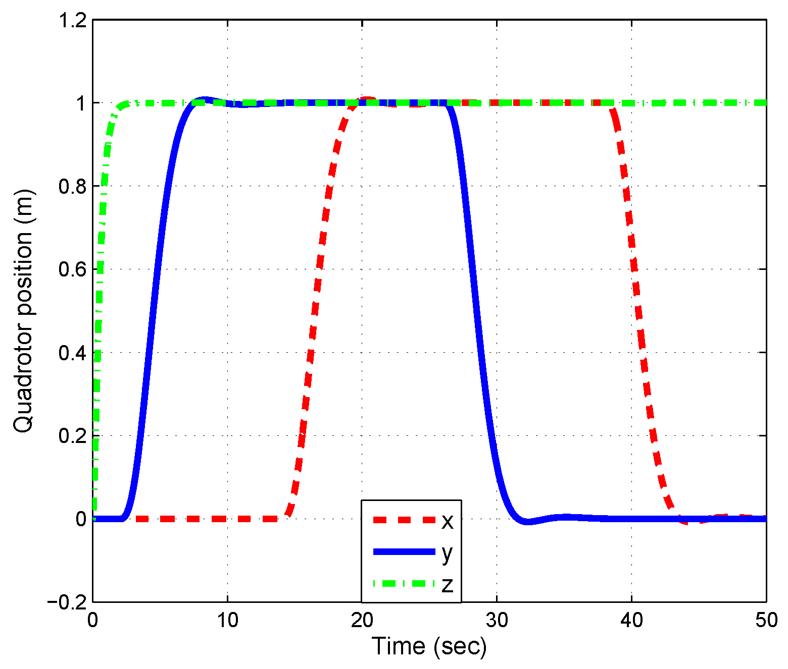
Figure 5 illustrates the x, y, and z positions of the vehicle during the validation. We can see that the position for each axis was stabilized according to the desired reference points. The position z was regulated in less than 2 s, the performance of the x and y positions dynamics were similar and were regulated in less than 5 s.

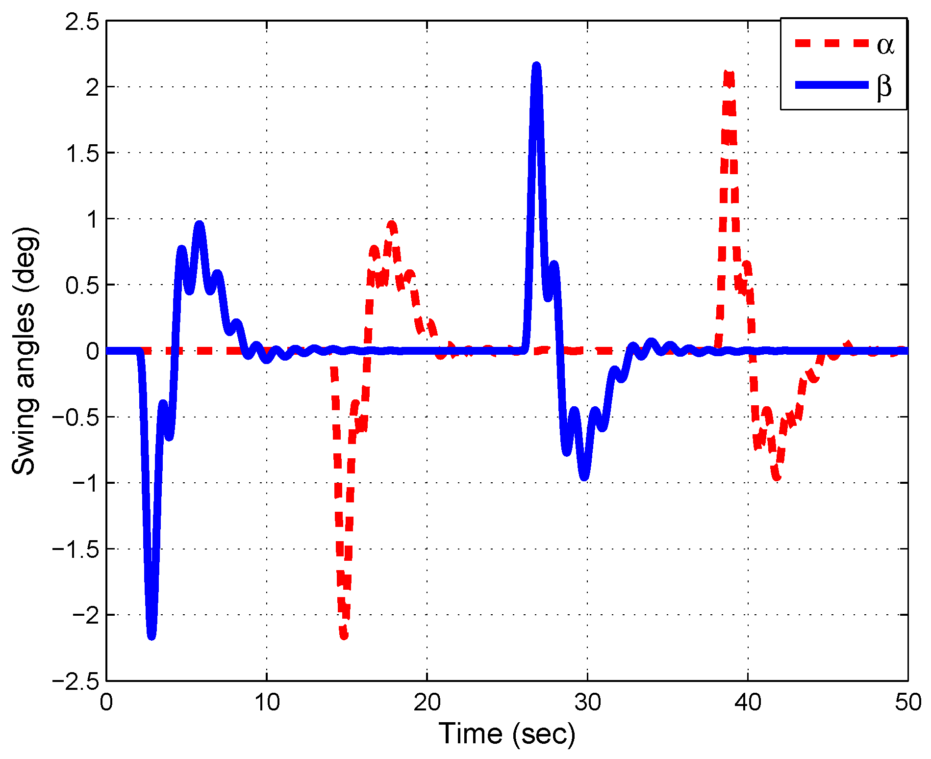
Figure 6 displays the payload swing angles α and β. It is clear that the proposed control law exhibited good performance, since the payload swing angles were regulated to $0^{\circ }$ at around 5 s and the maximum overshoot was ±$2.2^{\circ }$.

The simulation results of the feedback controller based on LMI (inner-loop of the system) show the quadrotor’s orientation dynamics in Figure 7. We can see that the attitude converged to the desired points with a null steady-state error. The evolution of the control inputs f, ${\tau }_{\psi }$, ${\tau }_{\theta }$, and ${\tau }_{\varphi }$ are presented in Figure 8. Finally, a three-dimensional view of the path followed by the vehicle is depicted in Figure 9.

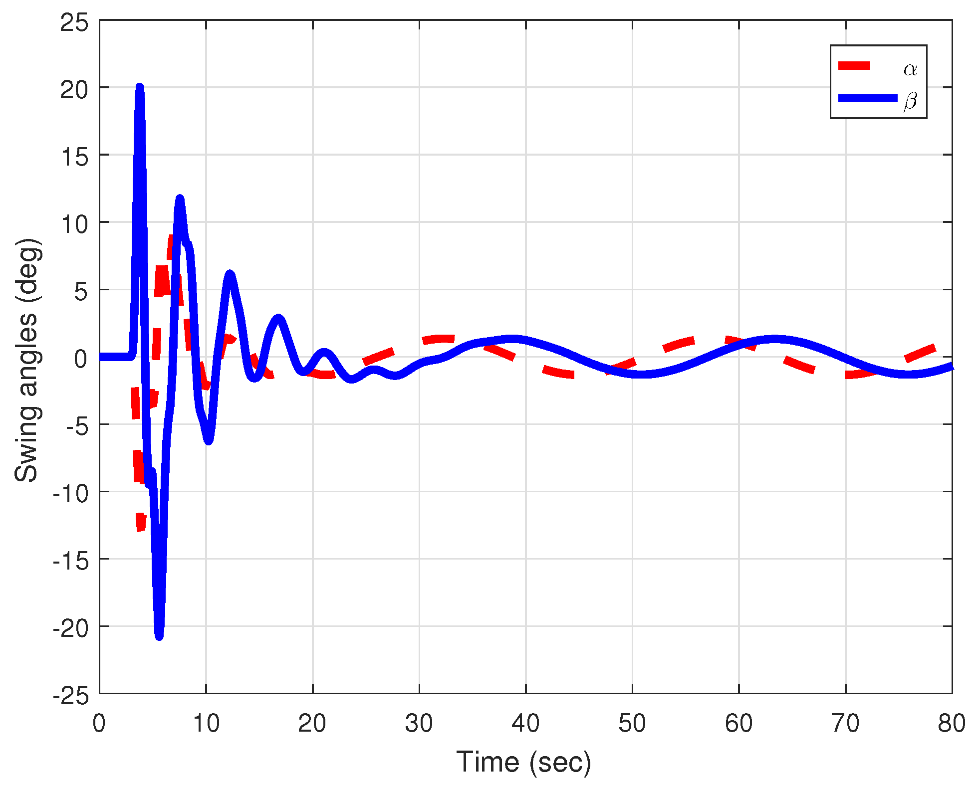
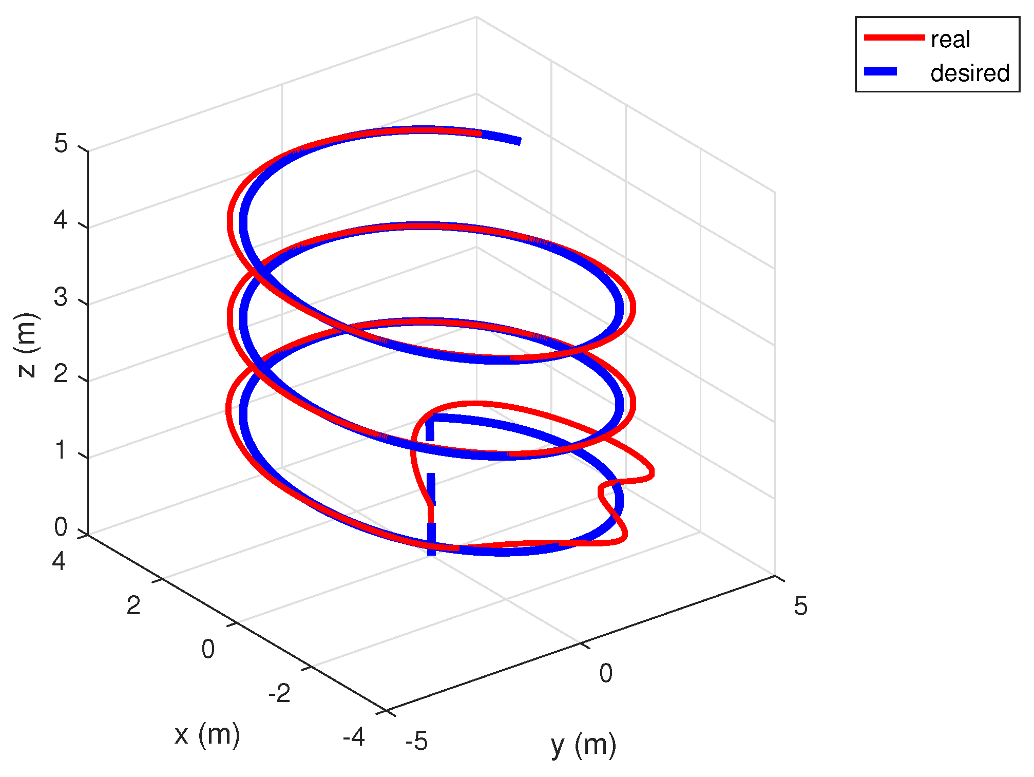
One more numerical experiment was carried out. Figure 10, Figure 11, Figure 12 and Figure 13 illustrate the tracking of an ascending circular trajectory to prove the efficiency of the proposed controller in a scenario that involves simultaneous variations of both α and β angles. These figures show that the proposed control strategy was capable of achieving accurate trajectory tracking since the aircraft converged to the reference trajectory while attenuating the swing angles of the payload.

In summary, these numerical experiments show that the proposed control scheme presented a satisfactory performance in position control and the attenuation of cable-suspended payload swing. It succeeded in transporting the payload to a desired position with attenuation of the oscillation angles. In contrast, the algorithm of [18] involves solving complicated partial differential equations for obtaining the control law, and they cannot be solved for the 3D case.

6. Conclusions

This work presents an energy-based control strategy and a nonlinear state feedback controller based on a linear matrix inequality to solve the problem of transporting a cable-suspended payload by an unmanned aerial vehicle. On one hand, a new methodology based on an LMI for stabilizing the orientation dynamics is proposed. The main contribution is that we can employ the proposed methodology for Lipschitz nonlinear systems with larger Lipschitz constants than other classical techniques based on LMIs. Moreover, the LMI-based controller results in a control algorithm with relative simplicity and guaranteed stability. In addition, the design of the LMI-based control takes into account physical limits of the system such as the maximum motor voltage or its rotation speed capability through the velocity and torque bounds which are used to calculate the Lipschitz constant, while with the energy-based control these limits are not part of the controller design. On the other hand, an energy-based control to stabilize the quadrotor’s translational dynamics and to attenuate the cable-suspended payload swing is designed in this work. This strategy is based on an energy approach and the passivity properties of the translational dynamics. Passivity-based control is employed, as this part of the system is underactuated. The main contribution is that the computation of excessive and complex partial differential equations is not needed to obtain the control law. The results showed an excellent performance of the proposed control scheme. Thus, the new approach achieves precise payload positioning with rapid oscillation attenuation.

Future work will extend the energy-based control method in order to consider variations in the payload. In addition, the methodology will be extended so that the linear matrix inequality can be replaced by an algebraic Riccati equation.

References

1. Bernard, M.; Kondak, K.; Maza, I.; Ollero, A. Autonomous transportation and deployment with aerial robots for search and rescue missions. J. Field Robot. 2011, 28, 914–931. [Google Scholar] [CrossRef]
2. Klausen, K.; Fossen, T.I.; Johansen, T.A. Nonlinear control of a multirotor UAV with suspended load. In Proceedings of the IEEE International Conference on Unmanned Aircraft Systems (ICUAS), Denver, CO, USA, 9–12 June 2015; pp. 176–184. [Google Scholar]
3. Sreenath, K.; Michael, N.; Kumar, V. Trajectory generation and control of a quadrotor with a cable-suspended load-a differentially-flat hybrid system. In Proceedings of the IEEE International Conference on Robotics and Automation (ICRA), Karlsruhe, Germany, 6–10 May 2013; pp. 4888–4895. [Google Scholar]
4. Sreenath, K.; Lee, T.; Kumar, V. Geometric control and differential flatness of a quadrotor UAV with a cable-suspended load. In Proceedings of the IEEE Conference on Decision and Control, Florence, Italy, 10–13 December 2013; pp. 2269–2274. [Google Scholar]
5. Nicotra, M.M.; Garone, E.; Naldi, R.; Marconi, L. Nested saturation control of an uav carrying a suspended load. In Proceedings of the IEEE American Control Conference, Portland, OR, USA, 4–6 June 2014; pp. 3585–3590. [Google Scholar]
6. Sadr, S.; Moosavian, S.A.A.; Zarafshan, P. Dynamics modeling and control of a quadrotor with swing load. J. Robot. 2014, 2014. [Google Scholar] [CrossRef]
7. Goodarzi, F.A.; Lee, D.; Lee, T. Geometric control of a quadrotor UAV transporting a payload connected via flexible cable. Int. J. Control. Autom. Syst. 2015, 13, 1486–1498. [Google Scholar] [CrossRef]
8. Dai, S.; Lee, T.; Bernstein, D.S. Adaptive control of a quadrotor UAV transporting a cable-suspended load with unknown mass. In Proceedings of the IEEE Conference on Decision and Control, Los Angeles, CA, USA, 15–17 December 2014; pp. 6149–6154. [Google Scholar]
9. Palunko, I.; Cruz, P.; Fierro, R. Agile load transportation: Safe and efficient load manipulation with aerial robots. IEEE Robot. Autom. Mag. 2012, 19, 69–79. [Google Scholar] [CrossRef]
10. Foehn, P.; Falanga, D.; Kuppuswamy, N.; Tedrake, R.; Scaramuzza, D. Fast Trajectory Optimization for Agile Quadrotor Maneuvers with a Cable-Suspended Payload. In Proceedings of the Robotics XIII: Science and Systems, Cambridge, MA, USA, 12–16 July 2017; pp. 1–10. [Google Scholar]
11. Qian, L.; Liu, H.H. Dynamics and control of a quadrotor with a cable suspended payload. In Proceedings of the IEEE Canadian Conference on Electrical and Computer Engineering (CCECE), Windsor, ON, Canada, 30 April–3 May 2017; pp. 1–4. [Google Scholar]
12. Rego, B.S.; Raffo, G.V. Suspended load path tracking control using a tilt-rotor UAV based on zonotopic state estimation. J. Frankl. Inst. 2019, 356, 1695–1729. [Google Scholar] [CrossRef]
13. Yi, K.; Liang, X.; He, Y.; Yang, L.; Han, J. Active-Model-Based Control for the Quadrotor Carrying a Changed Slung Load. Electronics 2019, 8, 461. [Google Scholar] [CrossRef]
14. Cabecinhas, D.; Cunha, R.; Silvestre, C. A trajectory tracking control law for a quadrotor with slung load. Automatica 2019, 106, 384–389. [Google Scholar] [CrossRef]
15. Weijers, M.; Carloni, R. Minimum swing control of a uav with a cable suspended load. In Robotics and Mechatronics; Technical Report; University of Twente: Enschede, The Netherlands, 2015. [Google Scholar]
16. Guerrero, M.; Mercado, D.; Lozano, R.; García, C. IDA-PBC methodology for a quadrotor uav transporting a cable-suspended payload. In Proceedings of the IEEE International Conference on Unmanned Aircraft Systems (ICUAS), Denver, CO, USA, 9–12 June 2015; pp. 470–476. [Google Scholar]
17. Guerrero, M.E.; Mercado, D.; Lozano, R.; García, C. Passivity based control for a quadrotor UAV transporting a cable-suspended payload with minimum swing. In Proceedings of the IEEE Conference on Decision and Control (CDC), Osaka, Japan, 15–18 December 2015; pp. 6718–6723. [Google Scholar]
18. Guerrero-Sánchez, M.E.; Mercado-Ravell, D.A.; Lozano, R.; García-Beltrán, C.D. Swing-attenuation for a quadrotor transporting a cable-suspended payload. ISA Trans. 2017, 68, 433–449. [Google Scholar]
19. Guerrero-Sánchez, M.E.; Abaunza, H.; Castillo, P.; Lozano, R.; García-Beltrán, C.D. Quadrotor Energy-Based Control Laws: A Unit-Quaternion Approach. J. Intell. Robot. Syst. 2017, 88, 347–377. [Google Scholar]
20. Ruggiero, F.; Cacace, J.; Sadeghian, H.; Lippiello, V. Passivity-based control of VToL UAVs with a momentum-based estimator of external wrench and unmodeled dynamics. Robot. Auton. Syst. 2015, 72, 139–151. [Google Scholar] [CrossRef]
21. Yüksel, B.; Secchi, C.; Bülthoff, H.H.; Franchi, A. Reshaping the physical properties of a quadrotor through IDA-PBC and its application to aerial physical interaction. In Proceedings of the IEEE International Conference on Robotics and Automation (ICRA), Hong Kong, China, 31 May–7 June 2014; pp. 6258–6265. [Google Scholar]
22. Acosta, J.Á.; Sanchez, M.; Ollero, A. Robust control of underactuated aerial manipulators via IDA-PBC. In Proceedings of the IEEE Conference on Decision and Control, Los Angeles, CA, USA, 15–17 December 2014; pp. 673–678. [Google Scholar]
23. Ryan, T.; Kim, H.J. LMI-based gain synthesis for simple robust quadrotor control. IEEE Trans. Autom. Sci. Eng. 2013, 10, 1173–1178. [Google Scholar] [CrossRef]
24. Yacef, F.; Bouhali, O.; Khebbache, H.; Boudjema, F. Takagi-sugeno model for quadrotor modelling and control using nonlinear state feedback controller. Int. J. Control. Theory Comput. Model. 2012, 2, 9–24. [Google Scholar] [CrossRef]
25. Khalil, H.K. Nonlinear Systems; Macmillan: New York, NY, USA, 2002. [Google Scholar]
26. Phanomchoeng, G.; Rajamani, R. Observer design for Lipschitz nonlinear systems using Riccati equations. In Proceedings of the IEEE American Control Conference, Baltimore, MD, USA, 30 June–2 July 2010; pp. 6060–6065. [Google Scholar]
Figure 1. Three-dimensional quadrotor with a cable-suspended payload.
Mathematics 07 01090 g001
Figure 2. Quadrotor attitude.
Mathematics 07 01090 g002
Figure 3. Control inputs.
Mathematics 07 01090 g003
Figure 4. Two-dimensional quadrotor with a cable-suspended payload.
Mathematics 07 01090 g004
Figure 5. Quadrotor position.
Mathematics 07 01090 g005
Figure 6. Swing angles.
Mathematics 07 01090 g006
Figure 7. Quadrotor attitude.
Mathematics 07 01090 g007
Figure 8. Control inputs.
Mathematics 07 01090 g008
Figure 9. Three-dimensional trajectory.
Mathematics 07 01090 g009
Figure 10. Quadrotor position.
Mathematics 07 01090 g010
Figure 11. Swing angles.
Mathematics 07 01090 g011
Figure 12. Quadrotor attitude.
Mathematics 07 01090 g012
Figure 13. >Three-dimensional trajectory.
Mathematics 07 01090 g013