Numerical Simulation of Feller’s Diffusion Equation

Abstract

This article is devoted to Feller’s diffusion equation, which arises naturally in probability and physics (e.g., wave turbulence theory). If discretized naively, this equation may represent serious numerical difficulties since the diffusion coefficient is practically unbounded and most of its solutions are weakly divergent at the origin. In order to overcome these difficulties, we reformulate this equation using some ideas from the Lagrangian fluid mechanics. This allows us to obtain a numerical scheme with a rather generous stability condition. Finally, the algorithm admits an elegant implementation, and the corresponding Matlab code is provided with this article under an open source license.

1. Introduction

The celebrated Feller equation was introduced in two seminal papers published by William Feller (1951/1952) in Annals of Mathematics [1,2]. These publications studied mathematically (and, henceforth, gave the name) the following equation (To be more accurate, W. Feller studied the following equation [1]:

$$p_t={\left[axu\right]}_{xx}-{\left[(c+bx)u\right]}_x,$$

where $a>0$ and $0<x<+\infty$.).

$$p_t+{\mathfrak{F}}_x=0,\mathfrak{F}(p,x,t)\stackrel{\mathrm{def}}{:=}-x·\left(\gamma p+\eta p_x\right),$$

(1)

where the subscripts $t$, x denote the partial derivatives, i.e., ${(·)}_t\stackrel{\mathrm{def}}{:=}{\displaystyle \frac{\partial (·)}{\partial t}}$, ${(·)}_x\stackrel{\mathrm{def}}{:=}{\displaystyle \frac{\partial (·)}{\partial x}}$. Two parameters $\gamma$ and $\eta >0$ can be time-dependent in some physical applications, even if in this study we assume they are constants, for the sake of simplicity (The numerical method we are going to propose can be straightforwardly generalized for this case when $\gamma =\gamma \left(t\right)$ and $\eta =\eta \left(t\right)$. Moreover, Feller’s processes with time-varying coefficients were studied recently in [3].). Equation (1) can be seen as the Fokker–Planck (or the forward Kolmogorov) equation, with $\gamma x$ being the drift and $\eta x$ being the diffusion coefficients (see [4] for more information on the Fokker–Planck equation). One can notice also that Equation (1) becomes singular at $x=0$ and $x=+\infty$. We remind that practically important solutions to Feller’s equation might be unbounded near $x=0$. In order to attempt solving Equation (1), one has to prescribe an initial condition $p(x,0)=p_0\left(x\right)$, presumably with a boundary condition at $x=0$. A popular choice is to prescribe the homogeneous boundary condition $p(0,t)\equiv 0$. For this choice of the boundary condition, it is not difficult to show that the Feller equation dynamics would preserve solution positivity provided that $p_0\left(x\right)⩾0$ (see Appendix A for a proof). The solution norm is also preserved (see Appendix B). Moreover, using the Laplace transform techniques, Feller has shown in [1] that the initial condition $p_0\left(x\right)$ determines uniquely the solution. In other words, no boundary condition at $x=0$ should be prescribed. This conclusion might appear, perhaps, to be counter-intuitive.

The great interest in Feller’s equation can be explained by its connection to Feller’s processes, which can be described by the following stochastic differential Langevin equation (The stochastic differential equations are understood in the sense of Itō.):

$$\mathrm{d}{X}_t=-\gamma X_t\mathrm{d}t+\sqrt{2\eta X_t}\mathrm{d}{\mathcal{W}}_t,$$

where ${\mathcal{W}}_t$ is the standard Wiener process, i.e., $\xi \left(t\right)\stackrel{\mathrm{def}}{:=}{\displaystyle \frac{\mathrm{d}{\mathcal{W}}_t}{\mathrm{d}t}}$ is zero-mean Gaussian white noise, i.e.,

$$\langle \xi \left(t\right)\rangle =0,\langle \xi \left(t\right)\xi \left(s\right)\rangle =\delta (t-s),$$

where the brackets $\langle ·\rangle$ denote an ensemble averaging operator. Then, the Probability Density Function (PDF) $p(x,t;x_0)$ of the process $X\left(t\right)$, i.e.,

$$\mathbb{P}\left\{x<X\left(t\right)<x+\mathrm{d}x|X\left(0\right)=x_0\right\}\equiv p(x,t;x_0)\mathrm{d}x,$$

satisfies Equation (1) with the following initial condition [5]:

$$p_0\left(x\right)=\delta (x-x_0),x_0\in {\mathbb{R}}^{+}.$$

The point $x=0$ is a singular boundary that the process $X\left(t\right)$ cannot cross. The Feller process is a continuous representation of branching and birth–death processes, which never attains negative values. This property makes it an ideal model not only in physical, but also in biological and social sciences [3,6,7].

As a general comprehensive reference on generalized Feller’s equations, we can mention the book [8]. Since at least a couple of years ago there has again been a growing interest for studying Equation (1). Some singular solutions to Feller’s equation with constant coefficients were constructed in [6] via spectral decompositions. Feller’s equation and Feller’s processes with time-varying coefficients were studied analytically (always using the Laplace transform) and asymptotically in [3].

The Feller (and Fokker–Planck) equation ’has already made its appearance in optical communications [9]. Recently, the Feller equation was derived in the context of the weakly interacting random waves dominated by four-wave interactions [10]. Wave Turbulence (We could define the Wave Turbulence (WT) as a physical and mathematical study of systems where random and coherent waves coexist and interact [11].) WT is a common name for such processes [11]. In WT, the Feller equation governs the PDF of squared Fourier wave amplitudes, i.e., $x\sim {\left|a\right|}^2$. In [10], some steady solutions to this equation with finite flux in the amplitude space were constructed (There is probably a misprint in ([10] p. 366). To obtain mathematically correct solutions, one has to define $n_k\stackrel{\mathrm{def}}{:=}{\displaystyle \frac{\eta }{\gamma }}$ on the line below Equation (14)). See also [12], Chapter 11 for a detailed discussion and interpretations. Recently, the Feller equation has been studied analytically in [13]. The authors applied the Laplace transform to it in space (this computation can be found even earlier in [1], Equation (3.1)) and the resulting non-homogeneous hyperbolic equation was solved using the method of characteristics along the lines presented in ([1], Section §3) (see ([1], Equation (3.9)) for the general analytical solution).

The behaviour of solutions $p(x,t)$ for large x describes the appearance probability of extreme waves. In the context of ocean waves, these extreme events are known as rogue (or freak) waves [14]. In the WT literature, any noticeable deviation from the Rayleigh distribution for $x\gg 1$ is referred to as the anomalous probability distribution of large amplitude waves [10]. For Gaussian wave fields, all statistical properties can be derived from the spectrum. However, the PDFs and other higher order moments are compulsory tools to study such deviations.

The present study focuses on the numerical discretization and simulation of Feller equation. The naive approach to solve this equation numerically encounters notorious difficulties. The first question that arises is what is the (numerical) boundary condition to be imposed at $x=0$? Moreover, one can notice that Equation (1) is posed on a semi-infinite domain. There are three main strategies to tackle this difficulty:

• Map ${\mathbb{R}}^{+}$ on a finite interval $[0,\ell ]$;
• Use spectral expansions on ${\mathbb{R}}^{+}$ (e.g., Laguerre or associated Laguerre polynomials);
• Replace (truncate) ${\mathbb{R}}^{+}$ to $[0,L]$, with $L\gg 1$.

In most studies, the latter option is retained by imposing some appropriate boundary conditions at the artificial boundary $x=L$. In our study, we shall propose a method that is able to handle the semi-infinite domain ${\mathbb{R}}^{+}$ without any truncations or simplifications. Finally, the diffusion coefficient in the Feller Equation (1) is unbounded. If the domain is truncated at $x=L$, then the diffusion coefficient takes the maximal value ${\nu }_{max}\stackrel{\mathrm{def}}{:=}\eta L\gg 1$, which depends on the truncation limit L and can become very large in practice. We remind also that explicit schemes for diffusion equations are subject to the so-called Courant–Friedrichs–Lewy (CFL) stability conditions [15]:

$$\Delta t⩽\frac{\Delta x^2}{2{\nu }_{max}}.$$

Taking into account the fact that ${\nu }_{max}$ can be arbitrarily large, no explicit scheme can be usable with Feller equation in practice. Moreover, the dynamics of the Feller equation spread over the space ${\mathbb{R}}^{+}$ even localized initial conditions. In general, one can show that the support of $p(x,t)$, $t>0$ is strictly larger (Using modern analytical techniques, it is possible to show even sharper results on the solution support, see e.g., [16].) than the one of $p(x,0)$. It is the so-called retention property. Thus, longer simulation times require larger domains. For all these reasons, it becomes clear that numerical discretization of the Feller equation requires special care.

In this study, we demonstrate how to overcome this assertion as well. The main idea behind our study is to bring together PDEs and Fluid Mechanics. First, we observe that the classical Eulerian description is not suitable for this equation, even if the problem is initially formulated in the Eulerian setting. Consequently, the Feller equation will be recast in special material or the so-called Lagrangian variables (It is known that both Eulerian and Lagrangian descriptions were proposed by the same person, Leonhard Euler), which make the resolution easier and naturally adaptive ([17], Chapter 7).

The present manuscript is organized as follows. The symmetry analysis of Equation (1) is performed in Section 2. Then, the governing equation is reformulated in Lagrangian variables in Section 3. The numerical results are presented in Section 4. Finally, the main conclusions and perspectives are outlined in Section 5.

2. Symmetry Analysis

In general, a linear PDE admits an infinity of conservation laws, with integrating multipliers being solutions to the adjoint PDE [18]. Here, we provide an interesting conservation law, which was found using the GeM Maple package [19]:

$${\left(E_1\left(-\frac{\gamma x}{\eta }\right)p\right)}_t+{}_{𝔊x}=0,$$

where $E_1\left(z\right)\stackrel{\mathrm{def}}{:=}{\int }_1^{+\infty }\frac{{\mathrm{e}}^{-tz}}{t}\mathrm{d}t$ is the so-called exponential integral function [20] and the flux 𝔊 is defined as

$$𝔊(x,p)\stackrel{\mathrm{def}}{:=}-\eta {\mathrm{e}}^{\frac{\gamma x}{\eta }}p-x\left(\gamma E_1\left(-\frac{\gamma x}{\eta }\right)p+\eta E_1\left(-\frac{\gamma x}{\eta }\right)p_x\right).$$

The symmetry group of point transformations can be computed using GeM package as well. The infinitesimal generators are given below:

$$\begin{array}{cc}\hfill {\mathsf{\xi }}_1& ={\mathcal{D}}_t,\hfill \\ \hfill {\mathsf{\xi }}_2& =p{\mathcal{D}}_p,\hfill \\ \hfill {\mathsf{\xi }}_3& =-\frac{{\mathrm{e}}^{-\gamma t}}{\gamma }{\mathcal{D}}_t+{\mathrm{e}}^{-\gamma t}x{\mathcal{D}}_x-{\mathrm{e}}^{-\gamma t}p{\mathcal{D}}_p,\hfill \\ \hfill {\mathsf{\xi }}_4& =\frac{{\mathrm{e}}^{\gamma t}}{\gamma }{\mathcal{D}}_t+{\mathrm{e}}^{\gamma t}x{\mathcal{D}}_x-\frac{\gamma {\mathrm{e}}^{\gamma t}}{\eta }xp{\mathcal{D}}_p,\hfill \\ \hfill {\mathsf{\xi }}_5& ={\mathrm{e}}^{(\gamma +c)t}ℳ\left(1+\frac{c}{\gamma },1,\frac{\gamma x}{\eta }\right){\mathrm{e}}^{-\frac{\gamma x}{\eta }}{\mathcal{D}}_p,\hfill \\ \hfill {\mathsf{\xi }}_6& ={\mathrm{e}}^{(\gamma +c)t}𝒰\left(1+\frac{c}{\gamma },1,\frac{\gamma x}{\eta }\right){\mathrm{e}}^{-\frac{\gamma x}{\eta }}{\mathcal{D}}_p,\hfill \end{array}$$

where $c\in \mathbb{R}$, $ℳ(a,b,z)$ and $𝒰(a,b,z)$ are Kummer special functions [20,21] (see also Appendix C). The corresponding point transformations, which map solutions of (1) into other solutions, can be readily obtained by integrating several ODE systems (we do not provide integration details here):

$$\left(t,x,p\right)\mapsto \left(t+{\mathsf{\epsilon }}_1,x,p\right),$$

$$\left(t,x,p\right)\mapsto \left(t,x,{\mathrm{e}}^{{\mathsf{\epsilon }}_2}p\right),$$

$$\left(t,x,p\right)\mapsto \left(\frac{1}{\gamma }ln\left({\mathsf{\epsilon }}_3\gamma +{\mathrm{e}}^{\gamma t}\right),\frac{{\mathrm{e}}^{\gamma t}}{{\mathsf{\epsilon }}_3\gamma +{\mathrm{e}}^{\gamma t}}x,\left(1+{\mathsf{\epsilon }}_3\gamma {\mathrm{e}}^{-\gamma t}\right)p\right),$$

$$\left(t,x,p\right)\mapsto \left(t-\frac{1}{\gamma }ln\left(1-{\mathsf{\epsilon }}_4\gamma {\mathrm{e}}^{\gamma t}\right),\frac{x}{1-{\mathsf{\epsilon }}_4\gamma {\mathrm{e}}^{\gamma t}},{\mathrm{e}}^{-{\displaystyle \frac{{\mathsf{\epsilon }}_4{\gamma }^{2}x{\mathrm{e}}^{\gamma t}}{\eta (1-{\mathsf{\epsilon }}_4\gamma {\mathrm{e}}^{\gamma t})}}}·p\right),$$

$$\left(t,x,p\right)\mapsto \left(t,x,p+{\mathsf{\epsilon }}_5ℳ\left(1+\frac{c}{\gamma },1,\frac{\gamma x}{\eta }\right){\mathrm{e}}^{-\frac{\gamma x}{\eta }+(\gamma +c)t}\right),$$

$$\left(t,x,p\right)\mapsto \left(t,x,p+{\mathsf{\epsilon }}_6𝒰\left(1+\frac{c}{\gamma },1,\frac{\gamma x}{\eta }\right){\mathrm{e}}^{-\frac{\gamma x}{\eta }+(\gamma +c)t}\right).$$

The first symmetry is the time translation. The second one is the scaling of the dependent variable (the governing equation is linear). Symmetries 3 and 4 are exponential scalings. Two last symmetries express the fact that we can always add to the solution a particular solution to the homogeneous equation to obtain another solution. For instance, the solutions invariant under time translations (${\mathsf{\xi }}_1$) are steady states and their general form is the following:

$$p\left(x\right)={\mathrm{e}}^{-\frac{\gamma x}{\eta }}\left({\mathcal{C}}_1{E}_1\left(-\frac{\gamma x}{\eta }\right)+{\mathcal{C}}_2\right),$$

(2)

where ${\mathcal{C}}_{1,2}$ are ‘arbitrary’ constants, which have to be determined from imposed conditions. Of course, they should be chosen so that the resulting steady solution is a valid probability distribution. It is not difficult to check that the imposed flux $\mathfrak{F}$ on the steady state solution is equal to ${\mathcal{C}}_1\eta$. Some properties of the exponential integral function are reminded in Appendix D.

We provide here also the general solutions invariant under the symmetry $\left({\mathsf{\xi }}_3\right)$:

$$p(x,t)=\left({\mathcal{C}}_2-{\mathcal{C}}_{1}t+\frac{{\mathcal{C}}_1}{\gamma }lnx\right){\mathrm{e}}^{-\frac{\gamma x}{\eta }}$$

and under symmetry $\left({\mathsf{\xi }}_4\right)$:

$$p(x,t)=\left({\mathcal{C}}_1+{\mathcal{C}}_{2}t+\frac{{\mathcal{C}}_2}{\gamma }lnx\right){\mathrm{e}}^{\gamma t}.$$

These solutions might be used, for example, to validate numerical codes.

Remark 1.

As a byproduct of this analysis, we obtain two new exact solutions to theFellerEquation (1):

$$\begin{array}{cc}\hfill p(x,t)& =ℳ\left(1+\frac{c}{\gamma },1,\frac{\gamma x}{\eta }\right){\mathrm{e}}^{-\frac{\gamma x}{\eta }+(\gamma +c)t},\hfill \\ \hfill p(x,t)& =𝒰\left(1+\frac{c}{\gamma },1,\frac{\gamma x}{\eta }\right){\mathrm{e}}^{-\frac{\gamma x}{\eta }+(\gamma +c)t},\hfill \end{array}$$

for some constant $c\in \mathbb{R}$.

3. Reformulation

By following the lines of ([17], Chapter 7), we are going to rewrite Feller’s Equation (1) with the so-called Lagrangian or material variables. The main advantage of this formulation is due to the fact that we can handle infinite domains without any truncations, transformations, etc. It becomes possible to carry computations in infinite domains. Our domain is semi-infinite ($x\in {\mathbb{R}}^{+}$), with the left boundary $x=0$ being a reflection point.

As the first step, we introduce the distribution function associated to the probability density $p(x,t)$:

$$\mathcal{P}(x,t)\stackrel{\mathrm{def}}{:=}{\int }_0^{x}p(\xi ,t)\mathrm{d}\xi .$$

(3)

The same can be done for the initial condition as well:

$${\mathcal{P}}_0\left(x\right)\stackrel{\mathrm{def}}{:=}{\int }_0^x{p}_0\left(\xi \right)\mathrm{d}\xi ,p_0\in W_{loc}^{1,1}\left({\mathbb{R}}^{+}\right).$$

We notice also two obvious properties of the function $\mathcal{P}(x,t)$:

$${\partial }_x\mathcal{P}(x,t)\equiv p(x,t),\underset{x\to 0}{lim}\mathcal{P}(x,t)=0,\underset{x\to +\infty }{lim}\mathcal{P}(x,t)=1.$$

Due to the positivity preservation property (see Appendix A), the function $\mathcal{P}(x,t)$ is nondecreasing in variable $x$. Thus, we can define its pseudo-inverse (This mapping is sometimes called in the literature as the reciprocal mapping [17] or an order preserving string [22].):

$$\mathcal{X}:[0,1]\times {\mathbb{R}}^{+}\mapsto {\mathbb{R}}^{+},$$

which can be computed as

$$\mathcal{X}(\overline{\mathcal{P}},t)\stackrel{\mathrm{def}}{:=}inf\{\xi \in {\mathbb{R}}^{+}|\mathcal{P}(\xi ,t)=\overline{\mathcal{P}}\}.$$

The operation of taking the pseudo-inverse can be also seen as a generalized hodograph transformation $(x,t;\mathcal{P})\mapsto (\mathcal{P},t;x)$ proposed presumably for the first time by Sir W.R. Hamilton [23]. Similarly, the initial condition does possess a pseudo-inverse as well:

$${\mathcal{X}}_0\left(\overline{\mathcal{P}}\right)\stackrel{\mathrm{def}}{:=}inf\{\xi \in {\mathbb{R}}^{+}|{\mathcal{P}}_0\left(\xi \right)=\overline{\mathcal{P}}\},$$

(4)

such that $\mathcal{X}(\overline{\mathcal{P}},0)\equiv {\mathcal{X}}_0\left(\overline{\mathcal{P}}\right)$.

If Feller Equation (1) holds in the sense of distributions, then the following equation holds as well:

$${\mathcal{P}}_t-x{\left[\gamma \mathcal{P}+\eta {\mathcal{P}}_x\right]}_x=0.$$

(5)

along with the initial condition

$$\mathcal{P}(x,0)={\mathcal{P}}_0\left(x\right).$$

Equation (5) can be readily obtained by exploiting the obvious property $p(x,t)={\partial }_x\mathcal{P}(x,t)$. In Appendix A, we show that zero value of the solution $p(x,t)$ is repulsive. Thus, ${\partial }_x\mathcal{P}(x,t)\equiv p(x,t)>0$, $\forall (x,t)\in {\left({\mathbb{R}}^{+}\right)}^2$. Thus, the implicit function theorem [24,25] guarantees the existence of derivatives of the inverse mapping $\mathcal{X}(\overline{\mathcal{P}},t)$. Let us compute them by differentiating, with respect to $\overline{\mathcal{P}}$ and t, the following obvious identity:

$$\mathcal{P}(\mathcal{X}(\overline{\mathcal{P}},t),t)\equiv \overline{\mathcal{P}}.$$

Thus, one can easily show that

$$\frac{\partial \mathcal{X}}{\partial \mathcal{P}}=\frac{1}{{\partial }_x\mathcal{P}},\frac{\partial \mathcal{X}}{\partial t}=-\frac{{\partial }_t\mathcal{P}}{{\partial }_x\mathcal{P}}.$$

Using these expressions of partial derivatives, we derive the following evolution equation for the inverse mapping $\mathcal{X}(\mathcal{P},·)$:

$${\left({\mathrm{e}}^{\gamma t}\mathcal{X}\right)}_t+\mathcal{X}·{\left[\eta {\mathrm{e}}^{\gamma t}{\left(\frac{\partial \mathcal{X}}{\partial \mathcal{P}}\right)}^{-1}\right]}_{\mathcal{P}}=0.$$

(6)

The last equation can be rewritten also by introducing a new dynamic variable:

$$\mathcal{Y}(\mathcal{P},t)\stackrel{\mathrm{def}}{:=}{\mathrm{e}}^{\gamma t}\mathcal{X}(\mathcal{P},t),\mathcal{Y}(\mathcal{P},0)\equiv \mathcal{X}(\mathcal{P},0).$$

(7)

It is not difficult to see that Equation (6) becomes

$${\mathcal{Y}}_t+\mathcal{Y}·{\left[\eta {\mathrm{e}}^{\gamma t}{\left(\frac{\partial \mathcal{Y}}{\partial \mathcal{P}}\right)}^{-1}\right]}_{\mathcal{P}}=0.$$

(8)

The last equation will be solved numerically in the following Section.

Remark 2.

We would like to underline the fact that, by our assumptions, $\frac{\partial \mathcal{Y}}{\partial \mathcal{P}}$ as well as $\frac{\partial \mathcal{X}}{\partial \mathcal{P}}$ cannot vanish. Thus, there is no problem in dividing by $\frac{\partial \mathcal{Y}}{\partial \mathcal{P}}$ in Equation (8).

Numerical Discretization

Earlier, we derived Equation (6), which governs the dynamics of the pseudo-inverse mapping $\mathcal{X}(\mathcal{P},·)$. The initial condition for Equation (6) is given by the pseudo-inverse (4) of the initial condition ${\mathcal{P}}_0\left(x\right)$. We discretize Equation (6) with an explicit discretization in time since it yields the most straightforward implementation.

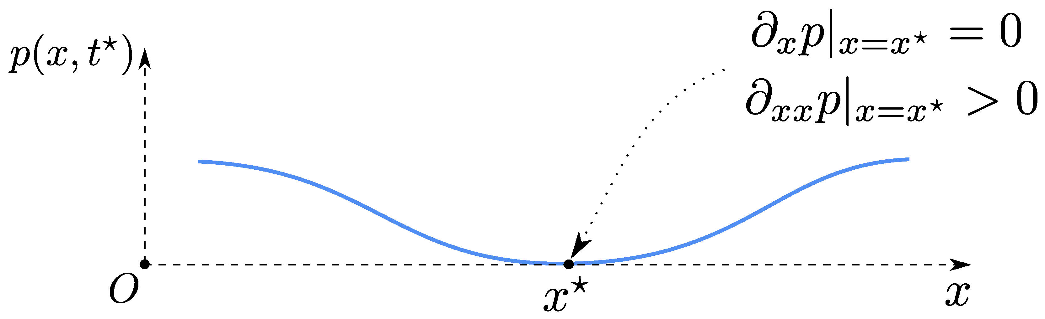
The first step in our algorithm consists of choosing the initial sampling interval. We make this choice depending on the provided initial condition. Typically, we want to sample only where it is needed. Thus, it seems reasonable to choose the initial segment $[0,{\ell }_0]$, with ${\ell }_0$ being the leftmost location such that

$$1-{\mathcal{P}}_0\left({\ell }_0\right)<\mathsf{tol}.$$

In simulations presented below, we chose $\mathsf{tol}\sim 𝒪\left({10}^{-5}\right)$. Then, we chose the initial sampling ${\left\{{\mathcal{X}}_k^0\right\}}_{k=0}^N\in [0,{\ell }_0]\subseteq {\mathbb{R}}^{+}$, with ${\mathcal{X}}_0^0=0$ and ${\mathcal{X}}_N^0={\ell }_0$. It is desirable that the initial sampling be adapted to the initial condition, since errors made initially cannot be corrected later. One of the possible strategies for the initial grid generation can be found in ([26], Section 2.3.1). We define also ${\mathcal{P}}_k={\mathcal{P}}_0\left({\mathcal{X}}_k^0\right)$. We stress that ${\left\{{\mathcal{P}}_k\right\}}_{k=0}^N$ stand for a discrete cumulative mass variable and, thus, they are time independent.

More generally, we introduce the following notation:

$${\mathcal{X}}_k^n\stackrel{\mathrm{def}}{:=}\mathcal{X}({\mathcal{P}}_k,t^n),k=0,1,\dots ,N,$$

with $t^n\stackrel{\mathrm{def}}{:=}n\Delta t$, $n\in \mathbb{N}$ and $\Delta t>0$ being a chosen time step. (We present our algorithm with a constant time step for the sake of simplicity. However, in realistic simulations presented in Section 4, the time step will be chosen adaptively and automatically to meet the stability and accuracy requirements prescribed by the user.) We introduce also similar notation for the dynamic variable:

$${\mathcal{Y}}_k^n\stackrel{\mathrm{def}}{:=}\mathcal{Y}({\mathcal{P}}_k,t^n),{\mathcal{Y}}_k^0\equiv {\mathcal{X}}_k^0,k=0,1,\dots ,N.$$

Now, we can state the fully discrete scheme for Equation (8):

$$\frac{{\mathcal{Y}}_k^{n+1}-{\mathcal{Y}}_k^n}{\Delta t}+\eta {\mathrm{e}}^{\gamma t^n}\frac{{\mathcal{Y}}_k^n}{\Delta {\mathcal{P}}_k}\left\{\frac{\Delta {\mathcal{P}}_{k+\frac{1}{2}}}{{\mathcal{Y}}_{k+1}^n-{\mathcal{Y}}_k^n}-\frac{\Delta {\mathcal{P}}_{k-\frac{1}{2}}}{{\mathcal{Y}}_k^n-{\mathcal{Y}}_{k-1}^n}\right\},$$

(9)

with $n⩾0$, $k=0,1,\dots ,N-1$ and

$$\Delta {\mathcal{P}}_{k+\frac{1}{2}}\stackrel{\mathrm{def}}{:=}{\mathcal{P}}_{k+1}-{\mathcal{P}}_k,\Delta {\mathcal{P}}_{k-\frac{1}{2}}\stackrel{\mathrm{def}}{:=}{\mathcal{P}}_k-{\mathcal{P}}_{k-1}.$$

The quantity $\Delta {\mathcal{P}}_k$ can be defined as the arithmetic or geometric mean of two neighbouring discretization steps $\Delta {\mathcal{P}}_{k\pm \frac{1}{2}}$:

$$\Delta {\mathcal{P}}_k\stackrel{\mathrm{def}}{:=}\frac{\Delta {\mathcal{P}}_{k+\frac{1}{2}}+\Delta {\mathcal{P}}_{k-\frac{1}{2}}}{2},\Delta {\mathcal{P}}_k\stackrel{\mathrm{def}}{:=}\sqrt{\Delta {\mathcal{P}}_{k+\frac{1}{2}}·\Delta {\mathcal{P}}_{k-\frac{1}{2}}}.$$

To be specific, in our code, we implemented the arithmetic mean. The fully discrete scheme can be easily rewritten under the form of a discrete dynamical system:

$${\mathcal{Y}}_k^{n+1}={\mathcal{Y}}_k^n-\eta \Delta t{\mathrm{e}}^{\gamma t^n}\frac{{\mathcal{Y}}_k^n}{\Delta {\mathcal{P}}_k}\left\{\frac{\Delta {\mathcal{P}}_{k+\frac{1}{2}}}{{\mathcal{Y}}_{k+1}^n-{\mathcal{Y}}_k^n}-\frac{\Delta {\mathcal{P}}_{k-\frac{1}{2}}}{{\mathcal{Y}}_k^n-{\mathcal{Y}}_{k-1}^n}\right\},n⩾0.$$

Remark 3.

We would like to say a few words about the implementation of boundary conditions. First of all, no boundary condition is required on the left side, where ${\mathcal{X}}_0^n={\mathcal{Y}}_0^n\equiv 0$. On the right boundary, we prefer to impose the infiniteNeumann-type boundary condition (i.e., $\frac{\partial \mathcal{Y}}{\partial \mathcal{P}}\to \infty$), which yields the exact ‘mass’ conservation at the discrete level as well. Namely, at the rightmost cell, we have the following fully discrete scheme:

$${\mathcal{Y}}_N^{n+1}={\mathcal{Y}}_N^n+\eta \Delta t{\mathrm{e}}^{\gamma t^n}\frac{{\mathcal{Y}}_N^n}{\Delta {\mathcal{P}}_N}·\frac{\Delta {\mathcal{P}}_{N-\frac{1}{2}}}{{\mathcal{Y}}_N^n-{\mathcal{Y}}_{N-1}^n},n⩾0,$$

with $\Delta {\mathcal{P}}_N\stackrel{\mathrm{def}}{:=}{\displaystyle \frac{{\mathcal{P}}_N-{\mathcal{P}}_{N-2}}{2}}$. As a result, we obtain the exact conservation of ‘mass’ at the discrete level:

$$\sum _{k=0}^N\Delta {\mathcal{P}}_k{\mathcal{X}}_k^n\equiv \sum _{k=0}^N\Delta {\mathcal{P}}_k{\mathcal{X}}_k^0,\forall n\in \mathbb{N}.$$

To summarize, our numerical strategy consists of the following steps:

• We compute the pseudo-inverse of the initial data $p_0\left(x\right)$ to obtain $\mathcal{X}(\mathcal{P},0)\equiv \mathcal{Y}(\mathcal{P},0)$.
• This initial condition $\mathcal{Y}(\mathcal{P},0)$ is evolved in (discrete) time using an explicit marching scheme in order to obtain numerical approximation to $\mathcal{Y}(\mathcal{P},t)$, $t>0$.
• The variable $\mathcal{X}(\mathcal{P},t)$ is recovered by inverting (7), i.e.,

  $$\mathcal{X}(\mathcal{P},t)={\mathrm{e}}^{-\gamma t}\mathcal{Y}(\mathcal{P},t).$$
• Thanks to (3), we can deduce the values of $p\left(\mathcal{X}(\mathcal{P},t),t\right)\in [0,1]$ by applying a favorite finite difference formula (In our code, we employed the simplest forward finite differences, and it led satisfactory results. This point can be easily improved when necessary.).

Working with the pseudo-inverse allows us to overcome the issue of the retention phenomenon, which manifests as the expanding support of $p(x,t)$ for positive (and possibly large) times $t>0$, $t\gg 1$, since the computational domain was transformed to $[0,1]$. This method is the Lagrangian counterpart of the moving mesh technique in the Eulerian setting [26,27].

A simple Matlab code, which implements the scheme we described above, is freely available for reader’s convenience at [28].

4. Numerical Results

In this Section, we validate and illustrate the application of the proposed algorithm on several examples. However, first, we begin with a straightforward validation test. The only difference with the proposed algorithm above is that we are using a higher-order adaptive time stepping for our practical simulations. The explicit first-order scheme was used to simplify the presentation. In practice, much more sophisticated time steppers can be used. For instance, we shall employ the explicit embedded Dormand–Prince Runge–Kutta pair $(4,5)$ [29] implemented in Matlab under the ode45 routine [30]. Conceptually, this method is similar to the explicit Euler scheme presented above. It conserved all good properties we showed, but it provides additionally the higher accuracy order and totally automatic adaptivity of the time step, which matches very well with adaptive features of the Lagrangian scheme in space. The values of absolute and relative tolerances used in the time step choice are systematically reported below.

4.1. Steady State Preservation

In order to validate the numerical algorithm, we have at our disposal a family of steady state solutions (2). Hence, if we take such a solution as an initial condition, normally the algorithm has to keep it intact under the discretized dynamics. The parameters $\eta$, $\gamma$ of the equation, those of the steady solution, and numerical parameters used in our computation are reported in

Table 1. Numerical parameters used in the steady state computations.

Parameter	Value
Drift coefficient, $\gamma$	$1.0$
Diffusion coefficient, $\eta$	$1.0$
Integration constant, ${\mathcal{C}}_1$	$0.0$
Integration constant, ${\mathcal{C}}_2$	${\displaystyle \frac{\eta }{\gamma }}\equiv 1.0$
Final simulation time, T	$10.0$
Number of discretization points, N	500
Absolute tolerance, ${\mathsf{tol}}_{\mathrm{a}}$	${10}^{-5}$
Relative tolerance, ${\mathsf{tol}}_{\mathrm{r}}$	${10}^{-5}$

. The initial condition at $t=0$ along with the final state at $t=T$ are shown in Figure 1. Up to graphical resolution they coincide completely. We can easily check that during the whole simulation the points barely moved, i.e.,

$${\parallel \mathcal{X}(·,T)-\mathcal{X}(·,0)\parallel }_{\infty }\approx 0.008577\dots$$

We can check also other quantities. For instance, $\mathcal{P}(,t)$ is preserved up to the machine precision. If we reconstruct the probability distribution $p(x,t)$, we obtain

$${\parallel p(·,T)-p(·,0)\parallel }_{\infty }\approx 0.003051\dots$$

The last error comes essentially from the fact that we apply simple first-order finite difference to reconstruct the variable $p(x,t)$ from its primitive $\mathcal{P}(x,t)$. We can improve this point, but even this simple reconstruction seems to be consistent with the overall scheme accuracy. Thus, this example shows that our implementation of the proposed algorithm is also practically well-balanced [17], since steady state solutions are well preserved.

4.2. Transient Computations

In this Section, we present a couple of extra truly unsteady computations in order to illustrate the capabilities of our method. Namely, we shall simulate the probability distributions emerging from a family of initial conditions (normalized to have the following probability distribution):

$$p_0\left(x\right)=\frac{{\mathrm{e}}^{-\frac{x}{{\sigma }_1}}+{\mathrm{e}}^{-\frac{x-x_0}{{\sigma }_2}}}{{\sigma }_1+{\sigma }_2{\mathrm{e}}^{\frac{x_0}{{\sigma }_2}}}.$$

The primitive of the last distribution can be easily computed as well:

$$\mathcal{P}\left(x\right)=1-\frac{{\sigma }_1{\mathrm{e}}^{-\frac{x}{{\sigma }_1}}+{\sigma }_2{\mathrm{e}}^{-\frac{x-x_0}{{\sigma }_2}}}{{\sigma }_1+{\sigma }_2{\mathrm{e}}^{\frac{x_0}{{\sigma }_2}}}.$$

We design two different experiments in silico to show two completely different behaviour of solutions to Feller Equation (1) depending on the sign of the drift coefficient $\gamma$. These will constitute additional tests for the proposed numerical method. In both cases, the initial positions of particles are chosen according to the logarithmic distribution (logspace function in Matlab) on the segment $[0,20]$. This choice is made to represent more accurately the exponentially decaying initial condition since the errors made in the initial condition cannot be corrected in the dynamics.

4.2.1. Expanding Drift

If the drift coefficient $\gamma <0$, this term will cause Feller’s Equation (1) to transport information in the rightward direction. This situation is quite uncomfortable from the numerical point of view since the initial condition expands quickly towards the (positive) infinity. We submitted our method to this case. All numerical and physical parameters are provided in

Table 2. Numerical parameters used in unsteady computations.

Parameter	Expanding Experiment	Confining Experiment
Drift coefficient, $\gamma$	$-0.1$	$0.5$
Diffusion coefficient, $\eta$	$1.0$	$1.0$
Final simulation time, T	$3.0$	$12.0$
Number of discretization points, N	100	100
Initial condition parameter, ${\sigma }_1$	$2.0$	$2.0$
Initial condition parameter, ${\sigma }_2$	$1.0$	$1.0$
Initial condition parameter, $x_0$	$3.0$	$3.0$
Absolute tolerance, ${\mathsf{tol}}_{\mathrm{a}}$	${10}^{-5}$	${10}^{-5}$
Relative tolerance, ${\mathsf{tol}}_{\mathrm{r}}$	${10}^{-5}$	${10}^{-5}$

(the middle column). The initial condition along with the probability distribution at the end of our simulation are shown simultaneously in Figure 2a,b in Cartesian and semilogarithmic coordinates correspondingly. As expected, the support of the initial condition more than triples from $t=0$ to $t=T=3.0$. We remind that the diffusion and drift coefficients are proportional to x, and the scheme handles the growth of these terms automatically. The smooth decay of the solution on the semilogarithmic plot (see Figure 2b) shows the absence of any numerical instabilities. The trajectory of grid nodes is shown in Figure 2c. One can see that points follow the expansion of the solution. Nevertheless, they concentrate in the areas where the probability takes significant values.

4.2.2. Confining Drift

In the case of the positive drift coefficient $\gamma >0$, the Feller dynamics get even more interesting since we have two competing effects:

• Positive drift moving information towards the origin $x=0$;
• Diffusion spreading solution towards the positive infinity.

It might happen that both effects balance each other and result in a steady solution. Such a simulation is presented in this Section. The numerical and physical parameters are given in Table 2 (the right column). The initial condition along with the probability distribution at the end of our simulations are shown simultaneously in Figure 3a,b in Cartesian and semilogarithmic coordinates, respectively. The trajectories of grid nodes are shown in Figure 2c. One can see the rapid initial expansion stage, which is followed by a stabilization process, when we almost achieved the expected steady state. Again, the grid nodes trajectories show excellent adaptive features of the numerical scheme—at the end of the simulation, the relative density of nodes turns out to be preserved. The semilogarithmic plot shown in Figure 3b shows that the numerical solution is free of numerical instabilities. The obtained steady solution will be preserved by discrete dynamics thanks to the well-balanced property demonstrated in Section 4.1.

5. Discussion

Above, we presented some rationale about the discretization, existence, and uniqueness theory for Feller’s equation. The main conclusions and perspectives are outlined below.

5.1. Conclusions

The celebrated Feller equation was studied mathematically in two seminal papers published by William Feller (1951/1952) in Annals of Mathematics [1,2]. In particular, the uniqueness was shown in [2] without any boundary condition required at $x=0$. This result is notable and we use it in our study. The main goal of our work was to present an efficient numerical scheme, which is able to handle the unbounded diffusion inherent to Equation (1). Moreover, the retention phenomenon causes the solution support to expand all the time. Thus, if we wait a sufficiently long time, it will reach the computational domain boundaries (since ${\mathbb{R}}^{+}\ni x$ was truncated to a finite segment to make the in silico simulation possible). To overcome this difficulty, we proposed a simple and explicit Lagrangian scheme using the notion of the pseudo-inverse. In this way, we obtained a stable numerical scheme (under not so stringent stability conditions), which turns out to be naturally adaptive as well, since particles move together with the growing support (the rightmost particle position defines the support) and tend to concentrate where it is really needed. The performance of our scheme was illustrated in several examples. We share also the Matlab code so that anybody can check the claims we made above and use it to solve numerically the Feller equation in their applications: https://github.com/dutykh/Feller/.

5.2. Perspectives

All the numerical schemes and results presented in this paper were in one ‘spatial’ dimension. The Feller equation considered here is 1D as well. However, it seems interesting (regardless of the physical applications) to consider generalized Feller equations in higher space dimensions and to extend the proposed numerical strategy to the multidimensional case as well. Another possible extension direction consists of proposing higher-order schemes to capture numerical solutions with better accuracy with the same number of degrees of freedom. On the more theoretical side, we would like to obtain an alternative well-posedness theory for Feller equation by taking a continuous limit in our numerical scheme.

References

1. Feller, W. Two Singular Diffusion Problems. Ann. Math. 1951, 54, 173. [Google Scholar] [CrossRef]
2. Feller, W. The Parabolic Differential Equations and the Associated Semi-Groups of Transformations. Ann. Math. 1952, 55, 468. [Google Scholar] [CrossRef]
3. Masoliver, J. Nonstationary Feller process with time-varying coefficients. Phys. Rev. E 2016, 93, 012122. [Google Scholar] [CrossRef] [PubMed] [Green Version]
4. Risken, H.; Till, F. The Fokker-Planck Equation: Methods of Solution and Applications, 2nd ed.; Springer Series in Synergetics; Springer: Berlin/Heidelberg, Germany, 1996; Volume 18. [Google Scholar]
5. Gardiner, C. Handbook of Stochastic Methods: for Physics, Chemistry and the Natural Sciences, 3rd ed.; Springer: Berlin/Heidelberg, Germany, 2004. [Google Scholar]
6. Gan, X.; Waxman, D. Singular solution of the Feller diffusion equation via a spectral decomposition. Phys. Rev. E 2015, 91, 012123. [Google Scholar] [CrossRef] [PubMed]
7. Murray, J.D. Mathematical Biology: I. An Introduction; Springer: Berlin/Heidelberg, Germany, 2007. [Google Scholar]
8. Lehnikg, S.H. The Generalized Feller Equation and Related Topics; Longman Scientific & Technical: Harlow, Essex, UK, 1993. [Google Scholar]
9. McKinstrie, C.; Lakoba, T. Probability-density function for energy perturbations of isolated optical pulses. Opt. Express 2003, 11, 3628–3648. [Google Scholar] [CrossRef] [PubMed]
10. Choi, Y.; Lvov, Y.V.; Nazarenko, S.; Pokorni, B. Anomalous probability of large amplitudes in wave turbulence. Phys. Lett. A 2005, 339, 361–369. [Google Scholar] [CrossRef] [Green Version]
11. Zakharov, V.E.; Lvov, V.S.; Falkovich, G. Kolmogorov Spectra of Turbulence I. Wave Turbulence; Series in Nonlinear Dynamics; Springer: Berlin, Germany, 1992. [Google Scholar]
12. Nazarenko, S. Wave Turbulence; Springer Series Lecture Notes in Phyics; Springer: Berlin, Germany, 2011; Volume 825. [Google Scholar]
13. Choi, Y.; Jo, S.; Kwon, Y.-S.; Nazarenko, S. Nonstationary distributions of wave intensities in wave turbulence. J. Phys. A Math. Gen. 2017, 50, 355502. [Google Scholar] [CrossRef] [Green Version]
14. Dysthe, K.B.; Krogstad, H.E.; Muller, P. Oceanic rogue waves. Ann. Rev. Fluid Mech. 2008, 40, 287–310. [Google Scholar] [CrossRef]
15. Courant, R.; Friedrichs, K.; Lewy, H. Über die partiellen Differenzengleichungen der mathematischen Physik. Math. Ann. 1928, 100, 32–74. [Google Scholar] [CrossRef]
16. Carrillo, J.A.; Gualdani, M.P.; Toscani, G. Finite speed of propagation in porous media by mass transportation methods. C. R. Mathématique 2004, 338, 15–818. [Google Scholar] [CrossRef]
17. Gosse, L. Computing Qualitatively Correct Approximations of Balance Laws: Exponential-Fit, Well-Balanced and Asymptotic-Preserving, 1st ed.; Volume 2 of SIMAI Springer Series; Springer: Milan, Italy, 2013. [Google Scholar]
18. Bluman, G.W.; Cheviakov, A.F.; Anco, S.C. Applications of Symmetry Methods to Partial Differential Equations; Springer: New York, NY, USA, 2010. [Google Scholar]
19. Cheviakov, A.F. GeM software package for computation of symmetries and conservation laws of differential equations. Comput. Phys. Comm. 2007, 176, 48–61. [Google Scholar] [CrossRef]
20. Abramowitz, M.; Stegun, I.A. Handbook of Mathematical Functions; Dover Publications: Mineola, NY, USA, 1972. [Google Scholar]
21. Kummer, E.E. De integralibus quibusdam definitis et seriebus infinitis. J. Für Die Reine Und Angew. Math. 1837, 17, 228–242. [Google Scholar]
22. Brenier, Y. Order preserving vibrating strings and applications to electrodynamics and magnetohydrodynamics. Methods Appl. Anal. 2004, 11, 512–532. [Google Scholar] [CrossRef]
23. Hamilton, R.W. The Hodograph, or a New Method of Expressing in Symbolic Language the Newtonian Law of Attraction. Proc. R. Irish Acad. 1847, 3, 344–353. [Google Scholar]
24. Zorich, V.A. Mathematical Analysis I, 2nd ed.; Springer Verlag: Berlin/Heidelberg, Germany; New York, NY, USA, 2008. [Google Scholar]
25. Zorich, V.A. Mathematical Analysis II, 2nd ed.; Springer Verlag: Berlin/Heidelberg, Germany; New York, NY, USA, 2008. [Google Scholar]
26. Khakimzyanov, G.S.; Dutykh, D.; Mitsotakis, D.; Shokina, N.Y. Numerical simulation of conservation laws with moving grid nodes: Application to tsunami wave modelling. Geosciences 2019, 9, 197. [Google Scholar] [CrossRef]
27. Khakimzyanov, G.; Dutykh, D. On supraconvergence phenomenon for second order centered finite differences on non-uniform grids. J. Comput. Appl. Math. 2017, 326, 1–14. [Google Scholar] [CrossRef] [Green Version]
28. Dutykh, D. 2019. Available online: https://github.com/dutykh/Feller/ (accessed on 1 November 2019).
29. Dormand, J.R.; Prince, P.J. A family of embedded Runge-Kutta formulae. J. Comput. Appl. Math. 1980, 6, 19–26. [Google Scholar] [CrossRef] [Green Version]
30. Shampine, L.F.; Reichelt, M.W. The MATLAB ODE Suite. SIAM J. Sci. Comput. 1997, 18, 1–22. [Google Scholar] [CrossRef] [Green Version]
Figure 1. Comparison of a steady state solution of class (2) at t = 0 and at t = T = 10 . They are indistinguishable up to the graphical resolution, which validates the solver.
Mathematics 07 01067 g001
Figure 2. Numerical result of the expanding experiment with negative drift γ = 0.1 > 0 : (a) initial and terminal states of the numerical discretized solution; (b) initial and terminal states of the numerical discretized solution in semilogarithmic coordinates; and (c) trajectories of grid nodes. All numerical parameters for this computation are reported in Table 2 (middle column).
Mathematics 07 01067 g002aMathematics 07 01067 g002b
Figure 3. Numerical result of the confining experiment with positive drift γ = 0.5 > 0 : (a) initial and terminal states of the numerical discretized solution; (b) initial and terminal states of the numerical discretized solution in semilogarithmic coordinates; and (c) trajectories of grid nodes. All numerical parameters for this computation are reported in Table 2 (right column).
Mathematics 07 01067 g003