A Novel System Reliability Modeling of Hardware, Software, and Interactions of Hardware and Software

Abstract

In the past few decades, a great number of hardware and software reliability models have been proposed to address hardware failures in hardware subsystems and software failures in software subsystems, respectively. The interactions between hardware and software subsystems are often neglected in order to simplify reliability modeling, and hence, most existing reliability models assumed hardware subsystems and software subsystem are independent of each other. However, this may not be true in reality. In this study, system failures are classified into three categories, which are hardware failures, software failures, and hardware-software interaction failures. The main contribution of our research is that we further classify hardware-software interaction failures into two groups: software-induced hardware failures and hardware-induced software failures. A Markov-based unified system reliability modeling incorporating all three categories of system failures is developed in this research, which provides a novel and practical perspective to define system failures and further improve reliability prediction accuracy. Comparison of system reliability estimation between the reliability models with and without considering hardware-software interactions is elucidated in the numerical example. The impacts on system reliability prediction as the changes of transition parameters are also illustrated by the numerical examples.

1. Introduction

To model system reliability, most studies have considered partial of the system, hardware subsystem or software subsystem [1,2,3,4,5,6,7,8,9,10,11,12]. In the past few decades, a great number of reliability models in terms of hardware [1,2,3,4,5,6,7] and software [8,9,10,11,12] have been proposed in order to address hardware failures in hardware subsystems and software failures in software subsystems from various perspectives considering many critical applications, respectively. The interactions between hardware and software subsystems are often neglected for the sake of simplifying mathematical formulation, and hence, hardware and software subsystems are assumed as independent in most studies. However, this assumption may not be true in reality.

Several studies have shown the existence of the interactions between these two subsystems, hardware and software, in modern complex system applications [13,14,15,16,17,18,19,20,21]. The health status, e.g., the degradation and failure, of hardware components is one of the critical factors affecting the performance of software subsystems [16,19,20]. Accordingly, one of the significant reasons that cause the failure of software is the malfunction/failure of hardware platform where software is located in [21]. From the software error studies on the existing Multiple Virtual Storage operating system, Iyer and Velardi [13] discovered that nearly 35 percent of the observed software failures were related with to the hardware platform. Their software errors analysis procedures demonstrated a new methodology to evaluate the interactions between hardware subsystems and software subsystems, which are related with system reliability. Reported by MessageOne [14], in any given 12-month time period, 35 percent email outages were triggered by hardware failure of the server. They reported that the average downtime due to the hardware failure was 18.1 h. Goswami and Iyer [20] studied the software behaviors under hardware fault and introduced a simulation-based software model that facilitated application-specific dependability analysis that can be applied in the early product design stages.

On the other hand, given that software subsystems are embedded in the hardware platform, the execution of software significantly increases the likelihood of hardware failures’ creation and further propagation [15,18,19,21]. The input of hardware components is essentially a series of 0 and 1 signal alternation from software execution. Such signal alternations will cause the voltage change and current flows in microelectronic device, which act as electronic stresses on the hardware platform, and may further result in the physical damage, e.g., degradation and failure, of hardware components [15]. Thus, Huang et al. [15] studied the manifestations of hardware failures because of the operational usage resulting from various applications of software execution. Software operations on the semiconductor devices are formed as voltage changes and current flows. Thus, the usage will steadily lead to the degradation and failure of the materials of circuit device until the device cannot well-perform its designed functionality. Therefore, the interactions between hardware and software need to be addressed properly to model system reliability.

Only a few studies established the whole system reliability model considering both the hardware subsystem and software subsystem [22,23,24,25,26,27]. References [23,24,25] simply assumed that there is no interaction between hardware and software subsystems; thus, the proposed system reliability model considered these two subsystems to be independent of each other. Teng et al. [22] developed a unified system reliability model including hardware, software and hardware-software interaction, in which hardware-software interaction failures were identified by the Markov process. In particular, hardware-software interaction failures are defined as the software failures resulting from the degradation of hardware components. However, the impact of software execution on hardware subsystems is not incorporated and properly addressed. Park et al. [26] proposed a software reliability model, taking into account that some portion of software failures is hardware-related, in which the Weibull-based model was used to represent hardware-related software failures. Recently, Zeng et al. [27] proposed an analytical method to address reliability of non-repairable hardware-software co-design systems on affecting system health status such as degradation and failure by incorporating the interaction between these two subsystems. However, both references [26,27] considered hardware-software interaction failures to be hardware-related software failure, as defined in Teng et al. [22]. Thus, the impact of software execution on hardware needs to be considered as part of hardware-software interactions and properly addressed. As a result, system failures are categorized into three groups: hardware failures, software failures, and hardware-software interaction failures.

The main contribution of this paper is that we further classified one of the system failures, hardware-software interaction failures, into two groups: software-induced hardware failures and hardware-induced software failures. To the best of our knowledge, no other study has included the above-defined failure categories: hardware failures, software failures, and hardware-software interaction failures (software-induced hardware failures and hardware-induced software failures) to establish a system reliability model.

This paper is organized as follows. Section 2 presents the classification and definitions of system failures and then proposes a unified system reliability model based on the Markov process incorporating three main categories of system failures. Through the numerical examples, Section 3 compares the system reliability estimation between the system reliability models with and without considering hardware-software interactions and illustrates the impacts on system reliability prediction by changing one transition parameter at a time while keeps others as same. Section 4 concludes this research and further discusses the future research direction.

2. Proposed Markov-based Unified System Reliability Model

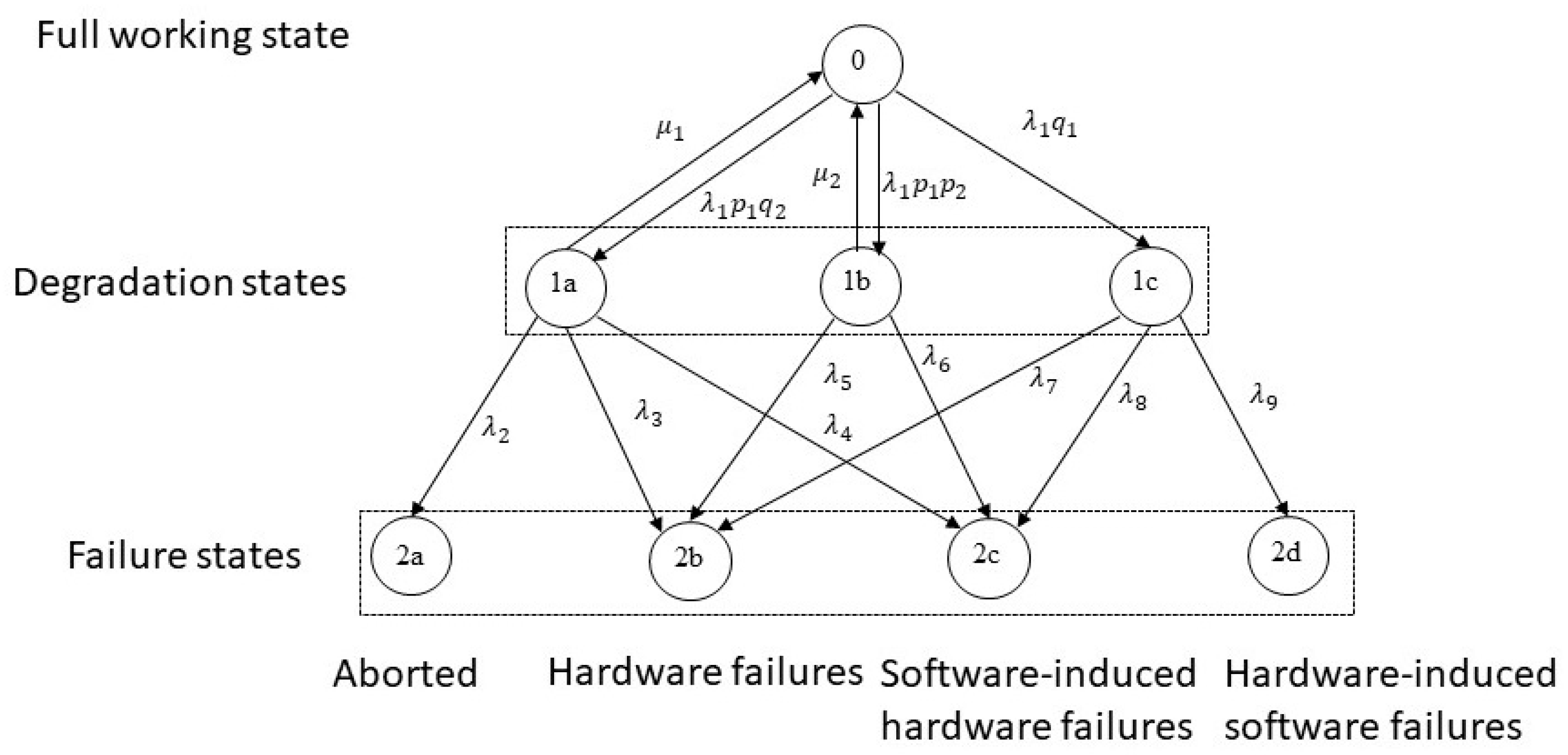
2.1. System Failures Classification

Complex system [28] refers to a system consists many components which may interact with each other. Many critical modern applications, such as communication systems and computing systems, are composed of many hardware and software components. In general, the failures of the whole system may be caused by the failures of one or more components. In this study, system failures are classified into three categories:

(1) Hardware failures [22,29,30] refer to a hardware component stops its designed function. Hardware failures are not able to be recovered by, for example, restarting the system after a certain period. Hardware failures are further classified as either total or partial hardware failures. In particular, total hardware failures, or hard failures by some studies [29,31], are catastrophic failures that cause complete cease of the designed function. Partial hardware failures, or soft failures [29,31], refer to the partial loss of the designed function, in which the hardware component may continue performing its designed function, but the system will under the degradation state. Overall, the system may continue working in a degradation state with partial hardware failures, but not with total hardware failures.

(2) Software failures [32] refer to the occurrence of an incorrect output that is triggered by a specific input because of the latent faults left in software program, e.g., design errors, that are unrelated with hardware components.

(3) The main contribution of this paper is that we particularly classified hardware-software interaction failures into two categories: software-induced hardware failures and hardware-induced software failures. Software-induced hardware failures were defined as hardware failures induced by the execution of embedded software system [15]. For example, the electronic stress induced by software execution may lead to the physical damage of hardware components. Hardware-induced software failures were defined as software failures resulting from a change in hardware configuration, which causes software operates in a different operational environment compared with the testing environment [22].

Transient hardware failures are also defined as one of the system failures in literature [15,22,29]. Generally, transient hardware failures are recovered by restarting the system since the disruption of the function usually caused by operation environment, such as high temperature, strong electromagnetic fluctuation. In this study, we did not incorporate transient hardware failures in reliability model.

2.2. Model Formulation

As discussed in the introduction, given that the interactions between hardware and software subsystems are often neglected, the novel Markov-based unified system reliability model was developed in this research by taking into account hardware failures, software failures, and hardware-software interaction failures, including software-induced hardware failures and hardware-induced software failures. The proposed Markov-based unified system reliability model has the following assumptions:

(1) System will fail if any of the failure happens, including hardware failures, software failures, and hardware-software interaction failures.

(2) Three categories of systems failures are independent of each other.

(3) The Weibull model is employed to model hardware reliability [29,30].

(4) Software fault detection process follows non-homogeneous Poisson process [32]. We consider the time to remove detected software faults to be negligible in this study.

(5) Three states are defined for hardware-software interactions: full working state (0), degradation states {state (1a), (1b), and (1c)}, and failure states {state (2a), (2b), (2c), (2d)}.

Hence, the Markov-based unified system reliability model is proposed follows:

$$R_{System}\left(t\right)=R_{Hardware}\left(t\right)R_{Software}\left(t\right)R_{H-S Interactions}\left(t\right)$$

(1)

where $R_{Hardware}\left(t\right)$, $R_{Software}\left(t\right)$, and $R_{H-S Interactions}\left(t\right)$ represent the reliability function of hardware subsystems, software subsystems, and hardware-software interactions, respectively.

In this study, the main concentration is on the reliability model development of hardware-software interactions. We employ the Markov process to represent the state transition of hardware-software interactions, as illustrated in Figure 1. As stated in model assumptions, three main states, full working state, degradation states, and failure states, and eight sub-states {0, 1a, 1b, 1c, 2a, 2b, 2c, 2d} are defined for hardware-software interactions. State (0) represents full working state, which means the system is under perfect working condition. Degradation state (1a) signifies that partial hardware failure is detected but it cannot be recovered by software. Degradation state (1b) signifies that partial hardware failure is detected and it can be recovered by software. Degradation state (1c) signifies that partial hardware failure is not detected. Failure state (2a) signifies execution abortion. Failures state (2b) signifies hardware failures. Failures state (2c) signifies software-induced hardware failures. Failure state (2d) signifies hardware-induced software failures.

The transition parameters described in Figure 1 are stated as follows. Hardware components can transit to degradation sate with degradation rate ${\lambda }_1$. The probability of detecting the partial hardware failures is $p_1$. Hence, the probability of not detecting the partially failed hardware is $q_1$, in which $q_1=1-p_1$. The probability of fixing the partial hardware failures through software is $p_2$. Hence, the probability that the partially failed hardware cannot be recovered through software is $q_2$, in which $q_2=1-p_2$.

The rate of fixing the partially failed hardware components, from state (1a) to full working status, state (0), through replacement is $u_1$. The rate of fixing the partially failed hardware components, from state (1b) to full working status, state (0), through replacement is $u_2$. No replacement will be performed if no failure is being detected.

The partially failed hardware can further transit from state (1a) to executing abortion, state (2a), with rate ${\lambda }_2$, hardware failures, state (2b), with rate ${\lambda }_3$, and software-induced hardware failures, state (2c), with rate ${\lambda }_4$. The partially failed hardware can further transit from state (1b) to hardware failures, state (2b), with rate ${\lambda }_5$, and software-induced hardware failures, state (2c), with rate ${\lambda }_6$. If the partially failed hardware is not being detected in the degradation states, it may further transit from state (1c) to hardware failures, state (2b), with rate ${\lambda }_7$, software-induced hardware failures, state (2c), with rate ${\lambda }_8$, and hardware-induced software failures, state (2d), with rate ${\lambda }_9$.

According to the model assumptions, the differential equations based on the Markov process [30,33,34] with $Q_i\left(t\right)$ denotes the probability of system being in the state $i$ at time $t$ are obtained as follows:

$$Q_0^{\prime }\left(t\right)=-{\lambda }_1{Q}_0\left(t\right)+{\mu }_1{Q}_{1a}\left(t\right)+{\mu }_2{Q}_{1b}\left(t\right)$$

(2)

$$Q_{1a}^{\prime }\left(t\right)={\lambda }_1{p}_1{q}_2{Q}_0\left(t\right)-\left({\mu }_1+{\lambda }_2+{\lambda }_3+{\lambda }_4\right)Q_{1a}\left(t\right)$$

(3)

$$Q_{1b}^{\prime }\left(t\right)={\lambda }_1{p}_1{p}_2{Q}_0\left(t\right)-\left({\mu }_2+{\lambda }_5+{\lambda }_6\right)Q_{1b}\left(t\right)$$

(4)

$$Q_{1c}^{\prime }\left(t\right)={\lambda }_1{q}_1{Q}_0\left(t\right)-\left({\lambda }_7+{\lambda }_8+{\lambda }_9\right)Q_{1c}\left(t\right)$$

(5)

$$Q_{2a}^{\prime }\left(t\right)={\lambda }_2{Q}_{1a}\left(t\right)$$

(6)

$$Q_{2b}^{\prime }\left(t\right)={\lambda }_3{Q}_{1a}\left(t\right)+{\lambda }_5{Q}_{1b}\left(t\right)+{\lambda }_7{Q}_{1c}\left(t\right)$$

(7)

$$Q_{2c}^{\prime }\left(t\right)={\lambda }_4{Q}_{1a}\left(t\right)+{\lambda }_6{Q}_{1b}\left(t\right)+{\lambda }_8{Q}_{1c}\left(t\right)$$

(8)

$$Q_{2d}^{\prime }\left(t\right)={\lambda }_9{Q}_{1c}\left(t\right)$$

(9)

We consider at time $t=0$ the probability of system being in full working state (0) is 1 and in degradation states {state (1a), (1b), and (1c)} and failure states {state (2a), (2b), (2c), and (2d)} are 0, respectively. Thus, the initial condition of the above differential Equations (2)–(9) will be given as $Q_0\left(0\right)=1$ and $Q_i\left(0\right)=0, i=1a, 1b, 1c, 2a, 2b,2c,2d$; the solutions of the differential Equations (2)–(9) of hardware-software interaction failures are obtained as follows:

$$Q_0\left(t\right)=\frac{\left(c_1+A_2\right)\left(c_1+A_1\right)}{\left(c_1-c_2\right)\left(c_1-c_3\right)}{e}^{c_{1}t}+\frac{\left(c_2+A_2\right)\left(c_2+A_1\right)}{\left(c_2-c_1\right)\left(c_2-c_3\right)}{e}^{c_{2}t}+\frac{\left(c_3+A_2\right)\left(c_3+A_1\right)}{\left(c_3-c_1\right)\left(c_3-c_2\right)}{e}^{c_{3}t}$$

$$Q_{1a}\left(t\right)={\lambda }_1{p}_1{q}_2\left[\frac{\left(c_1+A_2\right)}{\left(c_1-c_2\right)\left(c_1-c_3\right)}{e}^{c_{1}t}+\frac{\left(c_2+A_2\right)}{\left(c_2-c_1\right)\left(c_2-c_3\right)}{e}^{c_{2}t}+\frac{\left(c_3+A_2\right)}{\left(c_3-c_1\right)\left(c_3-c_2\right)}{e}^{c_{3}t}\right]$$

$$Q_{1b}\left(t\right)={\lambda }_1{p}_1{p}_2\left[\frac{\left(c_1+A_1\right)}{\left(c_1-c_2\right)\left(c_1-c_3\right)}{e}^{c_{1}t}+\frac{\left(c_2+A_1\right)}{\left(c_2-c_1\right)\left(c_2-c_3\right)}{e}^{c_{2}t}+\frac{\left(c_3+A_1\right)}{\left(c_3-c_1\right)\left(c_3-c_2\right)}{e}^{c_{3}t}\right]$$

$$\begin{array}{ll}{Q}_{1c}\left(t\right)=& {\lambda }_1{q}_1[\frac{\left(c_1+A_2\right)\left(c_1+A_1\right)}{\left(c_1-c_2\right)\left(c_1-c_3\right)\left(c_1+A_3\right)}{e}^{c_{1}t}+\frac{\left(c_2+A_2\right)\left(c_2+A_1\right)}{\left(c_2-c_1\right)\left(c_2-c_3\right)\left(c_2+A_3\right)}{e}^{c_{2}t}\\ & +\frac{\left(c_3+A_2\right)\left(c_3+A_1\right)}{\left(c_3-c_1\right)\left(c_3-c_2\right)\left(c_3+A_3\right)}{e}^{c_{3}t}-\frac{\left(A_3-A_2\right)\left(A_3-A_1\right)}{\left(A_3+c_1\right)\left(A_3+c_2\right)\left(A_3+c_3\right)}{e}^{-A_{3}t}]\end{array}$$

$$\begin{array}{ll}{Q}_{2a}\left(t\right)=& {\lambda }_1{\lambda }_2{p}_1{q}_2[\frac{-A_2}{c_1{c}_2{c}_3}+\frac{\left(c_1+A_2\right)}{c_1\left(c_1-c_2\right)\left(c_1-c_3\right)}{e}^{c_{1}t}+\frac{\left(c_2+A_2\right)}{c_2\left(c_2-c_1\right)\left(c_2-c_3\right)}{e}^{c_{2}t}\\ & +\frac{\left(c_3+A_2\right)}{c_3\left(c_3-c_1\right)\left(c_3-c_2\right)}{e}^{c_{3}t}]\end{array}$$

$$\begin{array}{ll}{Q}_{2b}\left(t\right)=& \frac{{\lambda }_1{\lambda }_3{p}_1{q}_2\left(c_1+A_2\right)+{\lambda }_1{\lambda }_5{p}_1{p}_2\left(c_1+A_1\right)}{c_1\left(c_1-c_2\right)\left(c_1-c_3\right)}{e}^{c_{1}t}\\ & +\frac{{\lambda }_1{\lambda }_3{p}_1{q}_2\left(c_2+A_2\right)+{\lambda }_1{\lambda }_5{p}_1{p}_2\left(c_1+A_1\right)}{c_2\left(c_2-c_1\right)\left(c_2-c_3\right)}{e}^{c_{2}t}\\ & +\frac{{\lambda }_1{\lambda }_3{p}_1{q}_2\left(c_3+A_2\right)+{\lambda }_1{\lambda }_5{p}_1{p}_2\left(c_3+A_1\right)}{c_3\left(c_3-c_1\right)\left(c_3-c_2\right)}{e}^{c_{3}t}\\ & -\frac{{\lambda }_1{\lambda }_3{p}_1{q}_2{A}_2+{\lambda }_1{\lambda }_5{p}_1{p}_2{A}_1}{c_1{c}_2{c}_3}\\ & +{\lambda }_1{\lambda }_7{q}_1[-\frac{A_1{A}_2}{c_1{c}_2{c}_3{A}_3}+\frac{\left(c_1+A_2\right)\left(c_1+A_1\right)}{c_1\left(c_1-c_2\right)\left(c_1-c_3\right)\left(c_1+A_3\right)}{e}^{c_{1}t}\\ & +\frac{\left(c_2+A_2\right)\left(c_2+A_1\right)}{c_2\left(c_2-c_1\right)\left(c_2-c_3\right)\left(c_2+A_3\right)}{e}^{c_{2}t}+\frac{\left(c_3+A_2\right)\left(c_3+A_1\right)}{c_3\left(c_3-c_1\right)\left(c_3-c_2\right)\left(c_3+A_3\right)}{e}^{c_{3}t}\\ & +\frac{\left(A_3-A_2\right)\left(A_3-A_1\right)}{A_3\left(A_3+c_1\right)\left(A_3+c_2\right)\left(A_3+c_3\right)}{e}^{-A_{3}t}]\end{array}$$

$$\begin{array}{ll}{Q}_{2c}\left(t\right)=& \frac{{\lambda }_1{\lambda }_4{p}_1{q}_2\left(c_1+A_2\right)+{\lambda }_1{\lambda }_6{p}_1{p}_2\left(c_1+A_1\right)}{c_1\left(c_1-c_2\right)\left(c_1-c_3\right)}{e}^{c_{1}t}\\ & +\frac{{\lambda }_1{\lambda }_4{p}_1{q}_2\left(c_2+A_2\right)+{\lambda }_1{\lambda }_6{p}_1{p}_2\left(c_2+A_1\right)}{c_2\left(c_2-c_1\right)\left(c_2-c_3\right)}{e}^{c_{2}t}\\ & +\frac{{\lambda }_1{\lambda }_4{p}_1{q}_2\left(c_3+A_2\right)+{\lambda }_1{\lambda }_6{p}_1{p}_2\left(c_3+A_1\right)}{c_3\left(c_3-c_1\right)\left(c_3-c_2\right)}{e}^{c_{3}t}\\ & -\frac{{\lambda }_1{\lambda }_4{p}_1{q}_2{A}_2+{\lambda }_1{\lambda }_6{p}_1{p}_2{A}_1}{c_1{c}_2{c}_3}\\ & +{\lambda }_1{\lambda }_8{q}_1[-\frac{A_1{A}_2}{c_1{c}_2{c}_3{A}_3}+\frac{\left(c_1+A_2\right)\left(c_1+A_1\right)}{c_1\left(c_1-c_2\right)\left(c_1-c_3\right)\left(c_1+A_3\right)}{e}^{c_{1}t}\\ & +\frac{\left(c_2+A_2\right)\left(c_2+A_1\right)}{c_2\left(c_2-c_1\right)\left(c_2-c_3\right)\left(c_2+A_3\right)}{e}^{c_{2}t}+\frac{\left(c_3+A_2\right)\left(c_3+A_1\right)}{c_3\left(c_3-c_1\right)\left(c_3-c_2\right)\left(c_3+A_3\right)}{e}^{c_{3}t}\\ & +\frac{\left(A_3-A_2\right)\left(A_3-A_1\right)}{A_3\left(A_3+c_1\right)\left(A_3+c_2\right)\left(A_3+c_3\right)}{e}^{-A_{3}t}]\end{array}$$

$$\begin{array}{ll}{Q}_{2d}\left(t\right)=& {\lambda }_1{\lambda }_9{q}_1[-\frac{A_1{A}_2}{c_1{c}_2{c}_3{A}_3}+\frac{\left(c_1+A_2\right)\left(c_1+A_1\right)}{c_1\left(c_1-c_2\right)\left(c_1-c_3\right)\left(c_1+A_3\right)}{e}^{c_{1}t}\\ & +\frac{\left(c_2+A_2\right)\left(c_2+A_1\right)}{c_2\left(c_2-c_1\right)\left(c_2-c_3\right)\left(c_2+A_3\right)}{e}^{c_{2}t}\\ & +\frac{\left(c_3+A_2\right)\left(c_3+A_1\right)}{c_3\left(c_3-c_1\right)\left(c_3-c_2\right)\left(c_3+A_3\right)}{e}^{c_{3}t}\\ & +\frac{\left(A_3-A_2\right)\left(A_3-A_1\right)}{A_3\left(A_3+c_1\right)\left(A_3+c_2\right)\left(A_3+c_3\right)}{e}^{-A_{3}t}]\end{array}$$

(10)

where $A_1={\mu }_1+{\lambda }_2+{\lambda }_3+{\lambda }_4$, $A_2={\mu }_2+{\lambda }_5+{\lambda }_6$, $A_3={\lambda }_7+{\lambda }_8+{\lambda }_9$. $c_1$, $c_2$, and $c_3$ are the roots of equation $\left(s+{\lambda }_1\right)\left(s+A_1\right)\left(s+A_2\right)-{\mu }_1{\lambda }_1{p}_1{q}_2\left(s+A_2\right)-{\mu }_2{\lambda }_1{p}_1{p}_2\left(s+A_1\right)=0$.

The working states include full working state (0) and degradation states (1a), (1b), and (1c). Hence, the reliability of hardware-software interactions is obtained as follows:

$$R_{H-SInteractions}\left(t\right)=Q_0\left(t\right)+Q_{1a}\left(t\right)+Q_{1b}\left(t\right)+Q_{1c}\left(t\right)$$

(11)

where $Q_0\left(t\right)$, $Q_{1a}\left(t\right)$, $Q_{1b}\left(t\right),$ and $Q_{1c}\left(t\right)$ are illustrated in Equation (10).

According to model assumptions, hardware reliability is elucidated by the Weibull model:

$$R_{Hardware}\left(t\right)=e^{-\lambda t^{\beta }}$$

(12)

where λ and β are the parameters of Weibull distribution.

Software fault detection and removal process are considered as a nonhomogeneous Poisson process. We also consider the time that software tester spent on removing detected software faults is negligible. In particular, software fault detection rate and the total number of software faults in the software program are considered as constants in this study; thus, G-O model [32,35] will be employed to estimate the expected number of detected software failures up to time $t$. G-O model [32,35] is shown below:

$$m\left(t\right)=a\left(1-e^{-bt}\right)$$

(13)

where $m\left(t\right)$ denotes the expected number of software failures up to time $t$. The constants $a$ and $b$ denote software fault detection rate and total number of software faults in the program, respectively.

Applying the G-O model given in Equation (13), the software reliability can be estimated for a time period $t$ given software startup time $x$ as follows:

$$R_{Software}\left(t|x\right)=e^{-\left[m\left(t+x\right)-m\left(x\right)\right]}=e^{a{e}^{-bx}\left(e^{-bt}-1\right)}$$

(14)

By substituting Equations (11), (12) and (14) to Equation (1), the proposed Markov-based unified system reliability model is obtained as follows:

$$R_{System}\left(t\right)=e^{-\lambda t^{\beta }}{e}^{a{e}^{-bx}\left(e^{-bt}-1\right)}\left[Q_0\left(t\right)+Q_{1a}\left(t\right)+Q_{1b}\left(t\right)+Q_{1c}\left(t\right)\right]$$

(15)

Note that this research mainly contributes on the reliability model development for hardware–software interactions. We do not develop new reliability model of hardware and software subsystems in this study. Hence, as an example, Weibull distribution and G-O model are, respectively, employed for modeling hardware reliability and software reliability to compare the entire system reliability with and without considering hardware-software interactions.

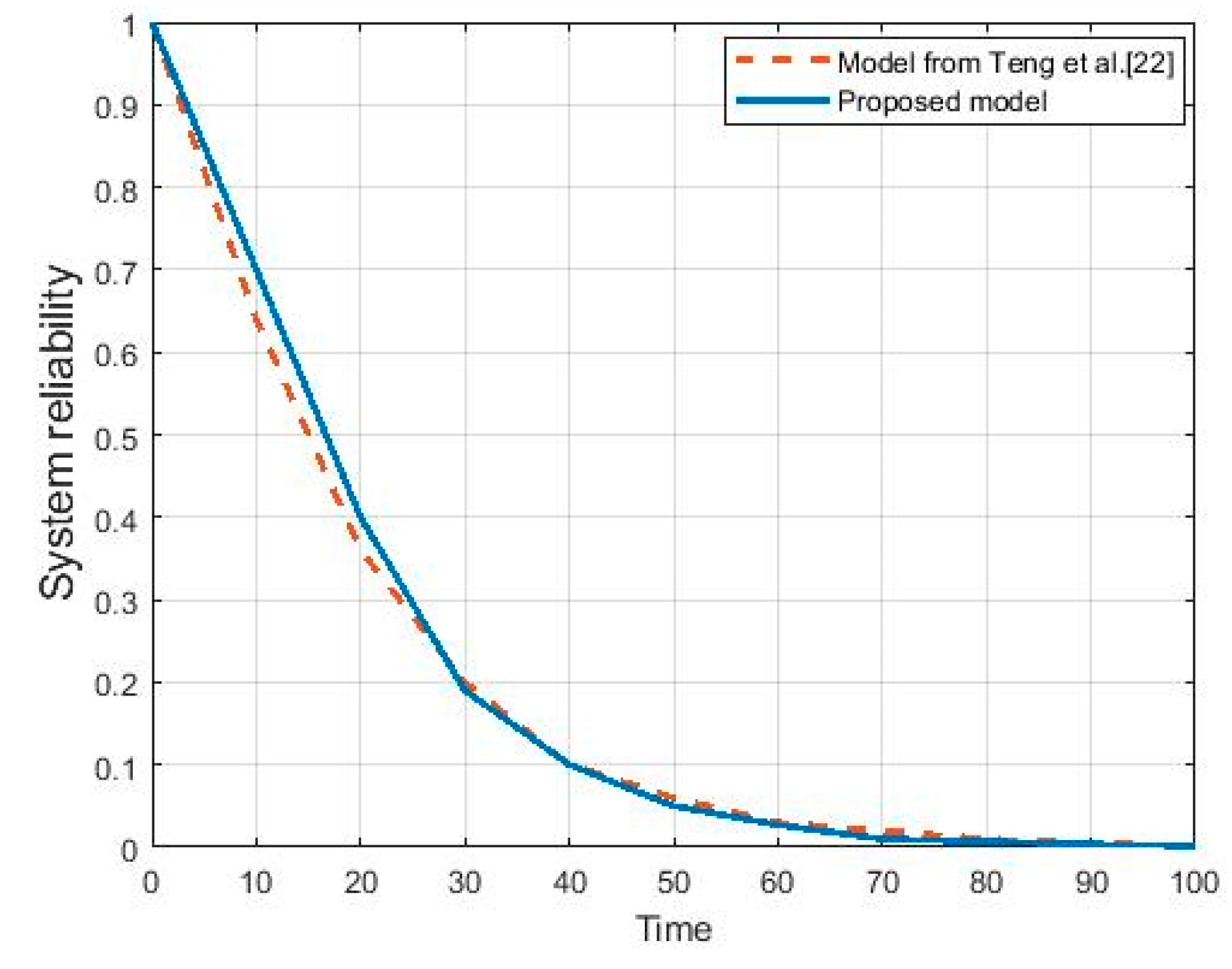
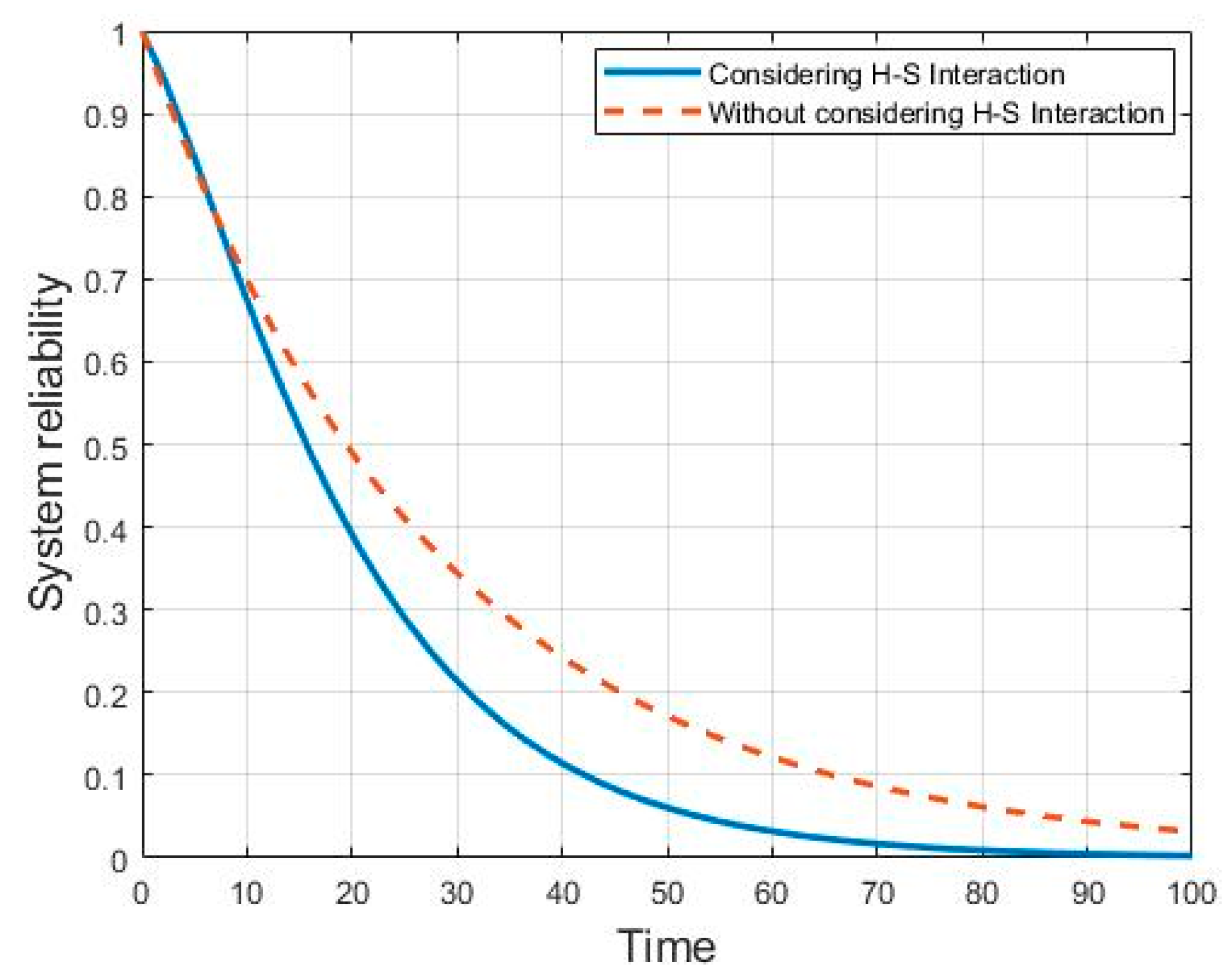
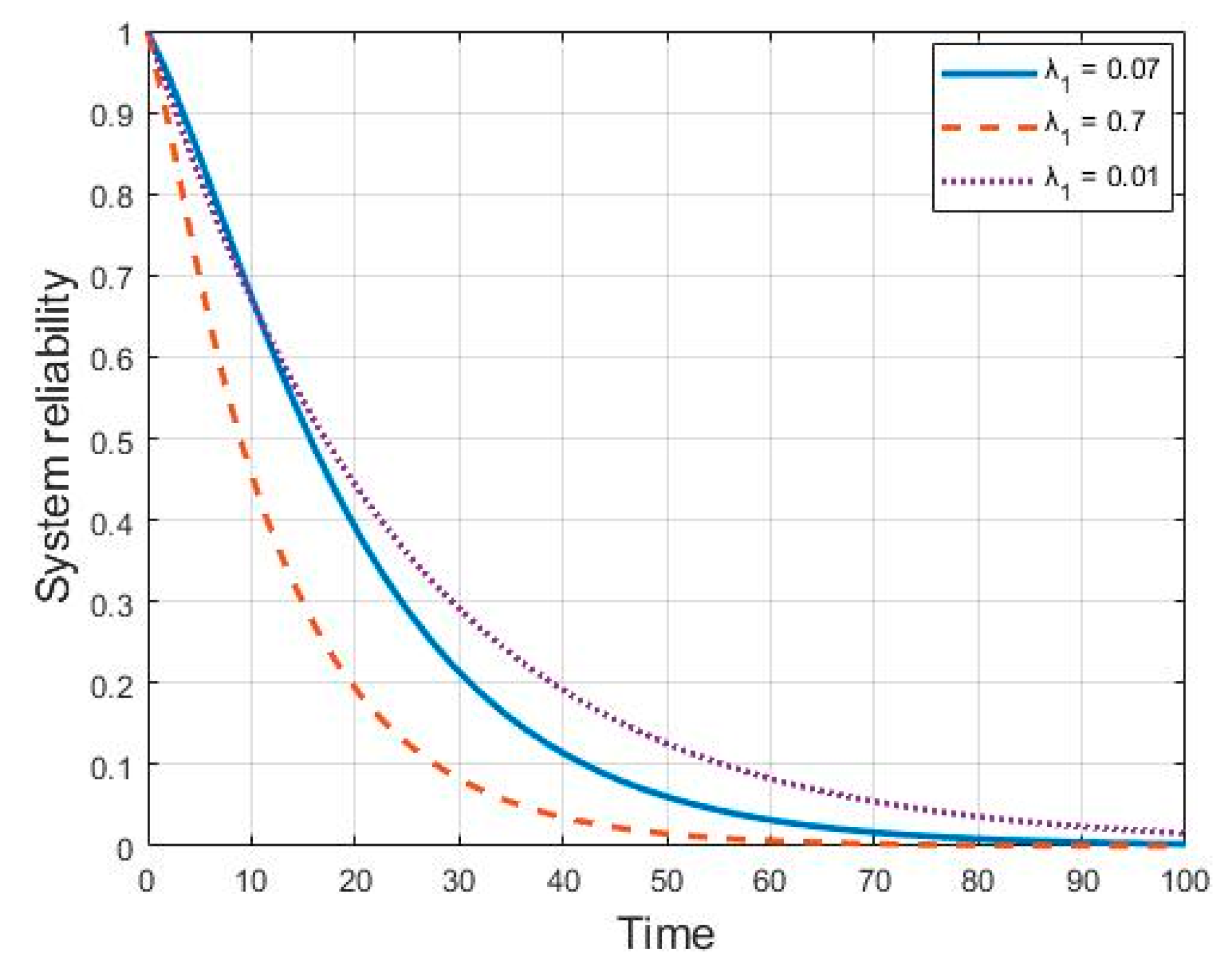
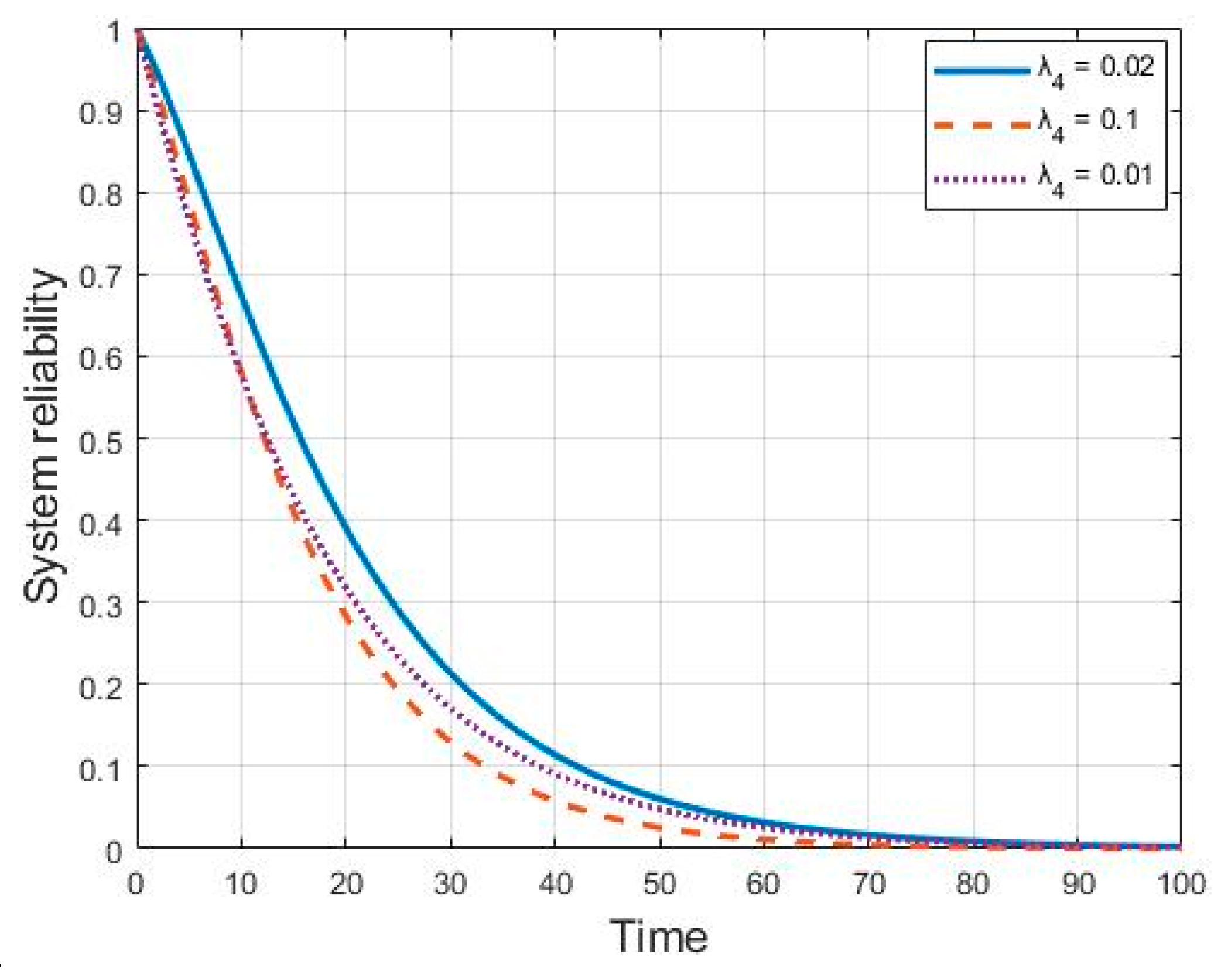
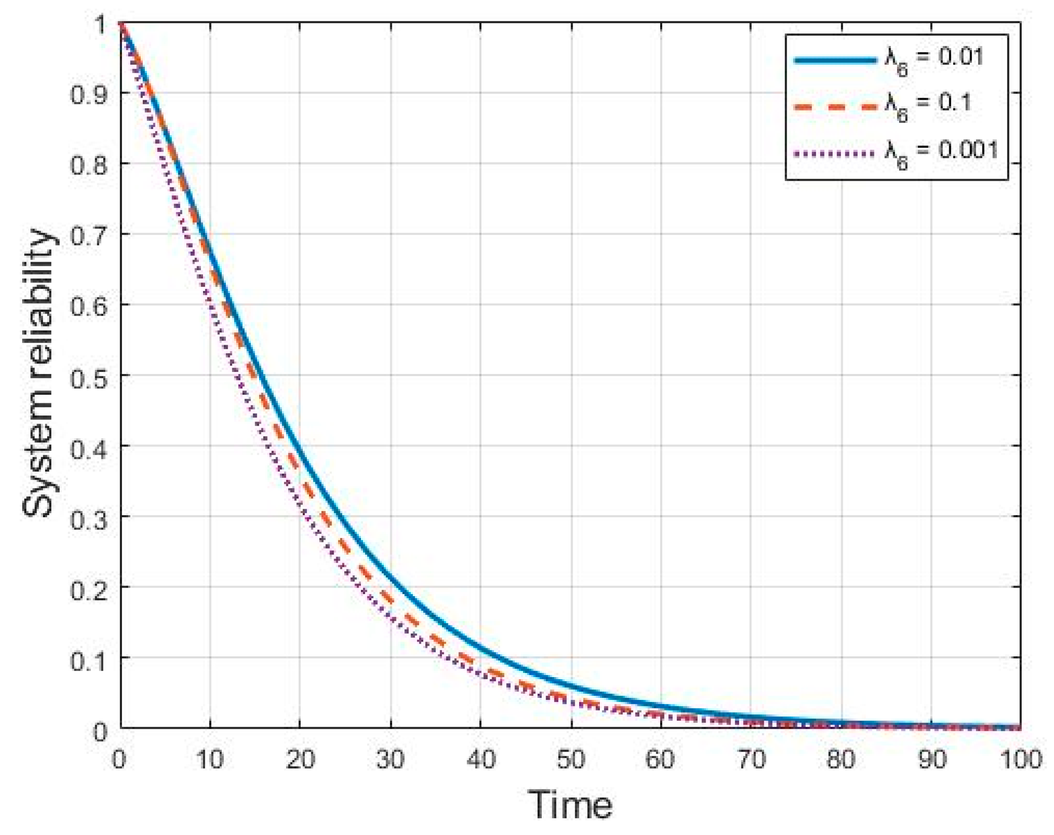
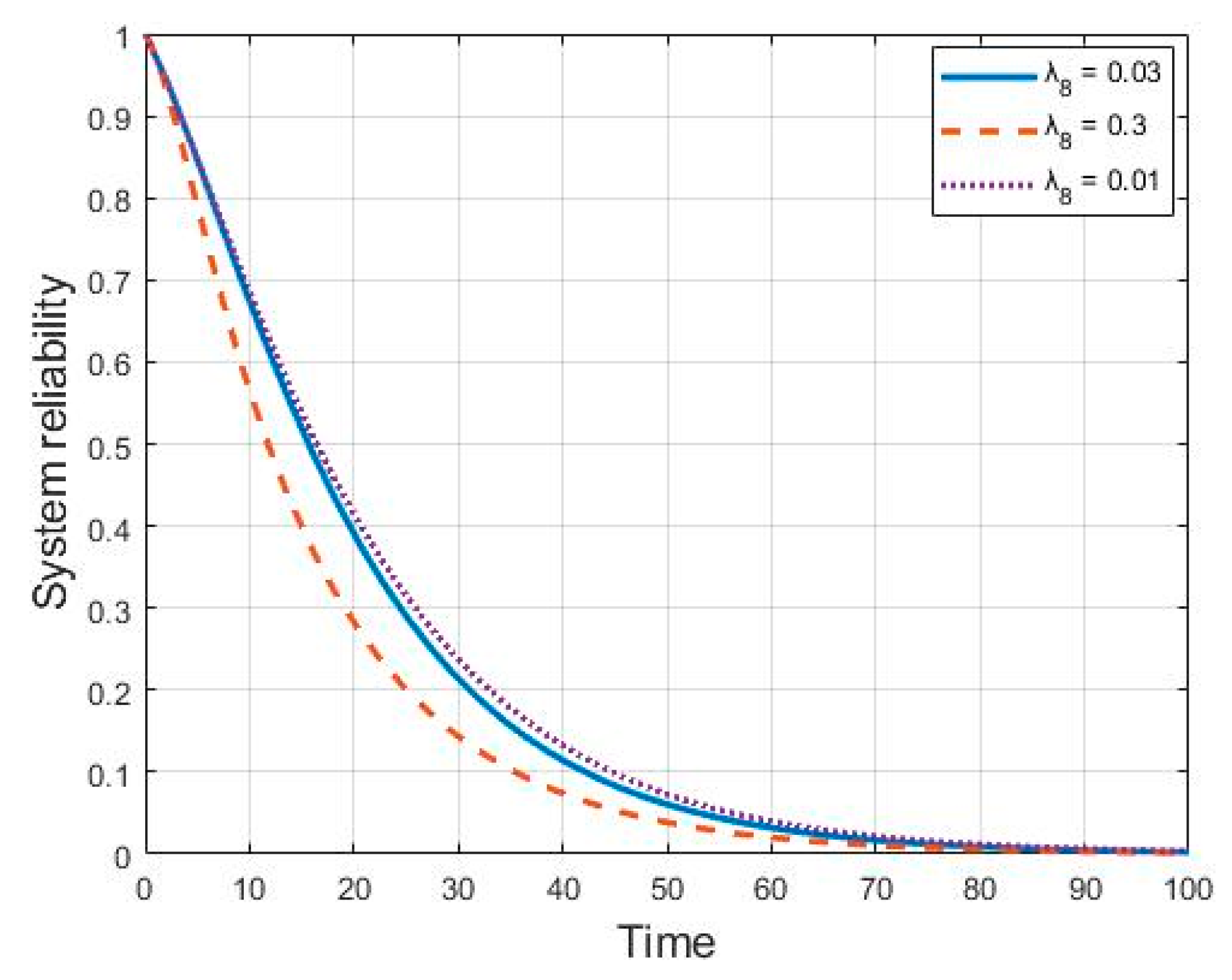
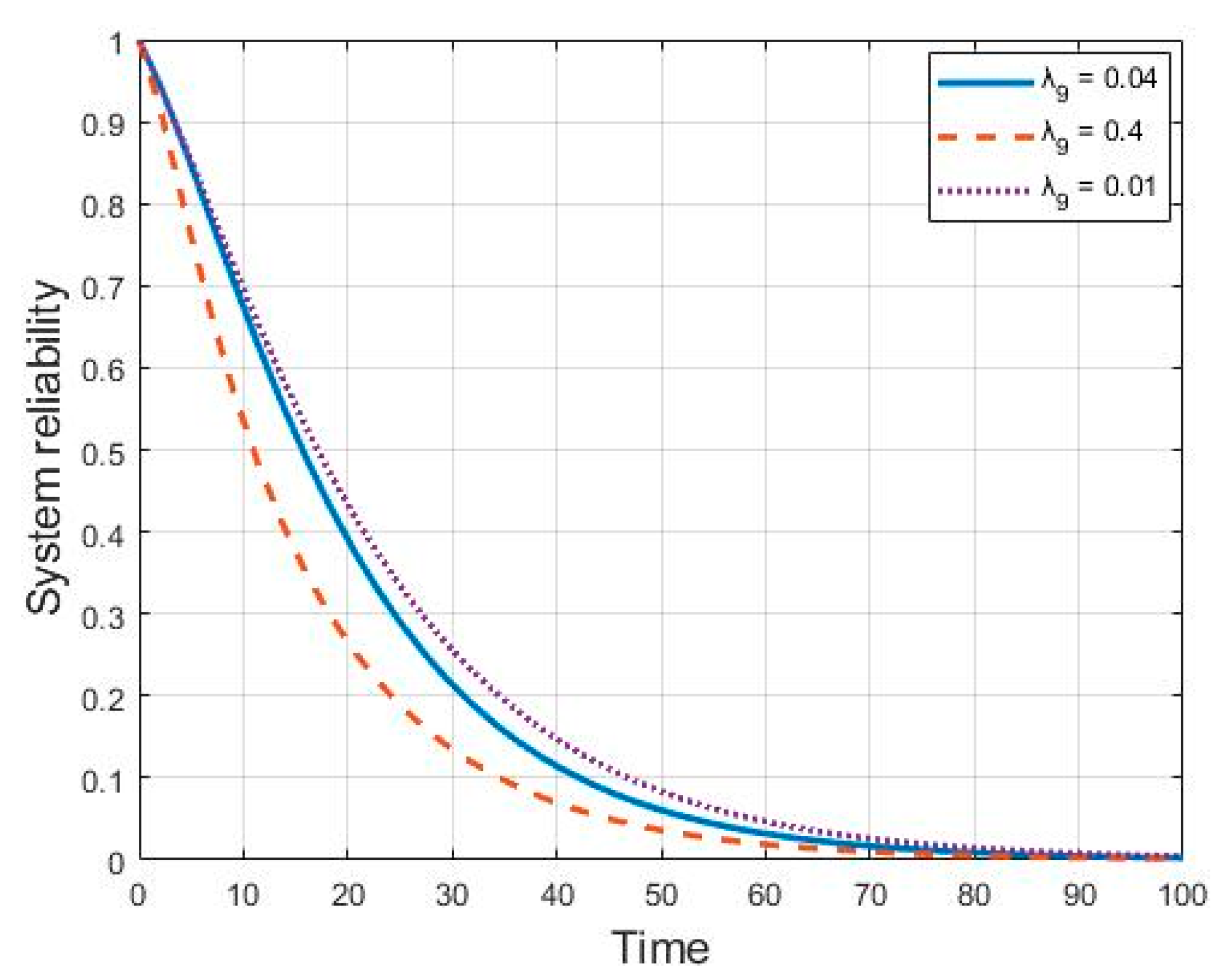
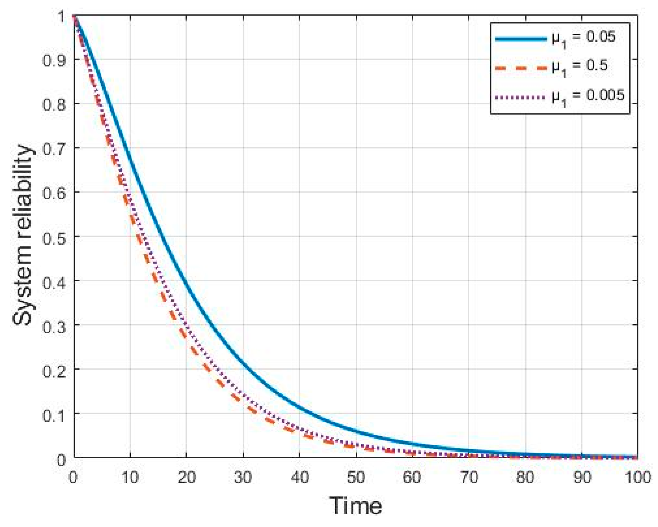
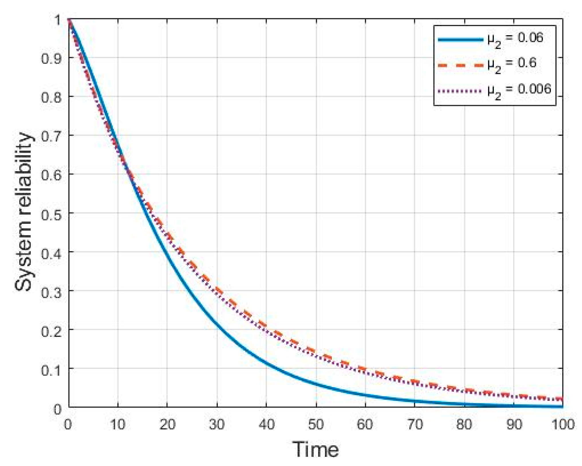
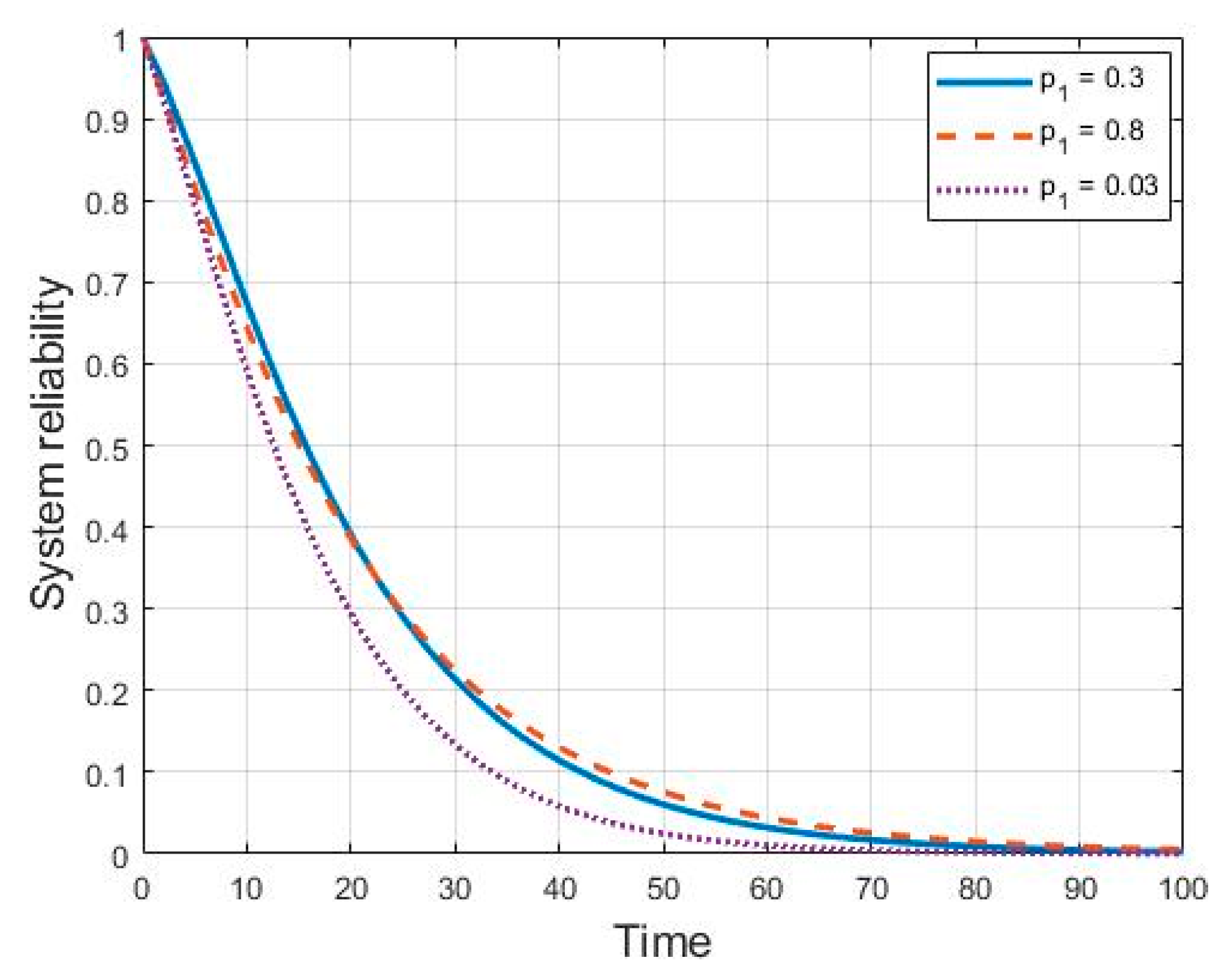
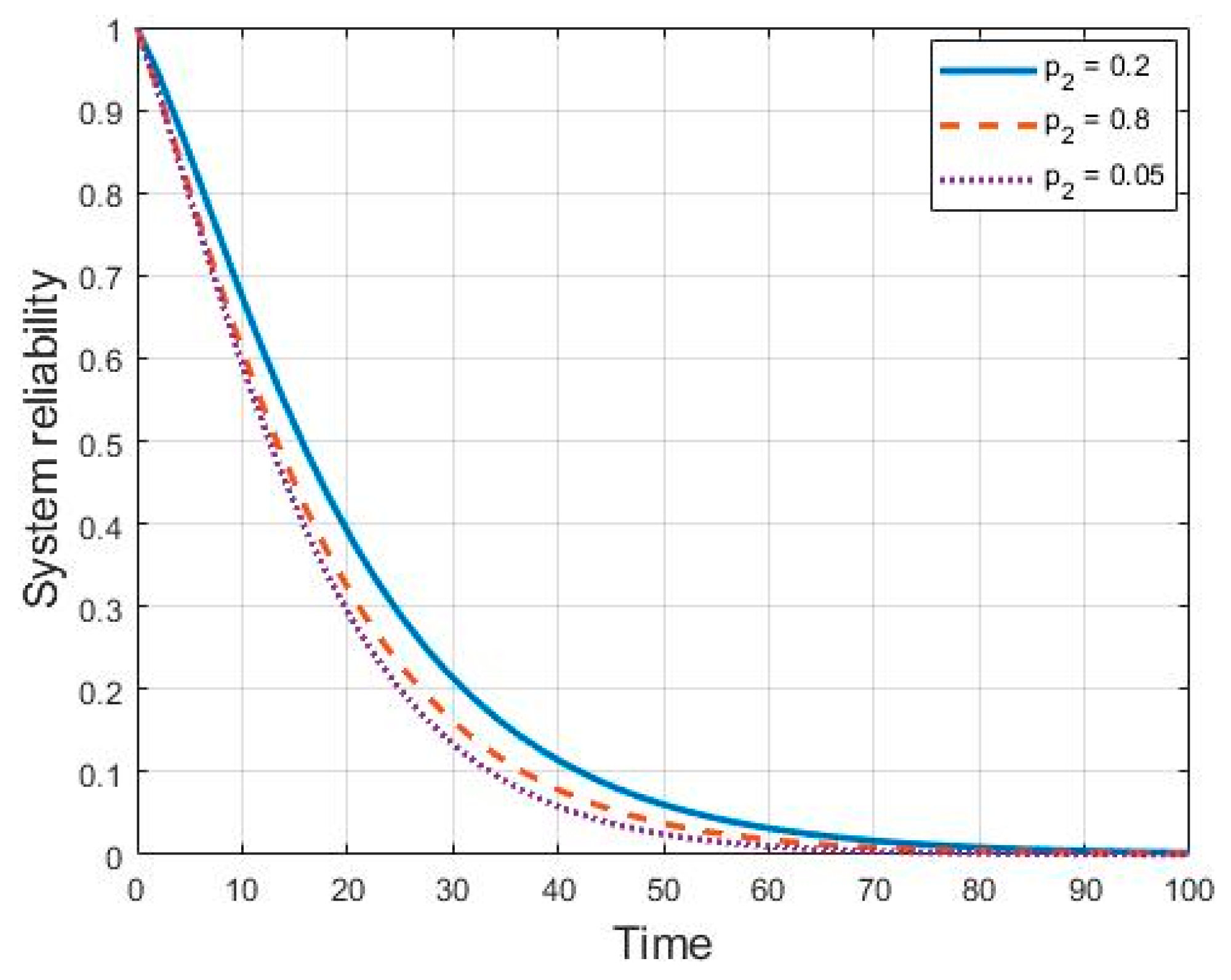
3. Numerical Examples

The state transition diagram of hardware-software interaction failures is shown in Figure 1. We are expecting the transitions from degradation states to execution abortion and hardware failures states can be neglected by considering $\min \left\{{\lambda }_i\right\}\gg {\lambda }_j, i=1, 4, 6, 8, 9, j=2, 3, 5,7$. Hence, we simplify the problem by taking ${\lambda }_j=0$. The transition parameters shown in Figure 1 are unknown. In practice, after collecting the testing/operation failure data, the parameter estimation methodologies, such as the maximum likelihood estimation and least squares method, can be employed to estimate these unknown parameters. However, we do not have the failure data from practice, since the proposed transaction diagram includes many degradation and failure states, which cause the transition rates to be very complicated to measure in the industry. It is vital to demonstrate the importance of considering such interactions between hardware and software subsystems (software-induced hardware failures and hardware-induced software failures) and the impacts on system reliability prediction as the changes of transition parameters. By taking the numerical examples illustrated in references [1,22,27] as references, we initially set up the transition parameters for the proposed Markov-based unified system reliability model as: $\lambda =0.006$, $\beta =1.09$, $a=30$, $b=0.001$, $x=10$, ${\lambda }_1=0.07$, ${\lambda }_4=0.02$, ${\lambda }_6=0.01$, ${\lambda }_8=0.03$, ${\lambda }_9=0.04$, ${\mu }_1=0.05$, ${\mu }_2=0.06$, $p_1=0.3$, and $p_2=0.2$, and then obtain the numerical values of $A_1, A_2, A_3, c_1, c_2, \mathrm{and} c_3$ stated in $Q_i\left(t\right)$, as described in Equation (10).

Given the initial parameter set, we are interested in the impacts on system reliability prediction as the transition parameters change. Time $t$ is set up as 100 in the numerical examples. The initial parameter set is ${\mathsf{\Theta }}_0$, as seen in

Table 1. Different transition parameter sets ${\mathsf{\Theta }}_{S_i-k}$.

Set	λ1	λ4	λ6	λ8	λ9	μ1	μ2	p1	p2
${\mathsf{\Theta }}_0$	0.07	0.02	0.01	0.03	0.04	0.05	0.06	0.3	0.2
${\mathsf{\Theta }}_{{\lambda }_{1}1}$	0.7	0.02	0.01	0.03	0.04	0.05	0.06	0.3	0.2
${\mathsf{\Theta }}_{{\lambda }_{1}2}$	0.01	0.02	0.01	0.03	0.04	0.05	0.06	0.3	0.2
${\mathsf{\Theta }}_{{\lambda }_{4}1}$	0.07	0.1	0.01	0.03	0.04	0.05	0.06	0.3	0.2
${\mathsf{\Theta }}_{{\lambda }_{4}2}$	0.07	0.01	0.01	0.03	0.04	0.05	0.06	0.3	0.2
${\mathsf{\Theta }}_{{\lambda }_{6}1}$	0.07	0.02	0.1	0.03	0.04	0.05	0.06	0.3	0.2
${\mathsf{\Theta }}_{{\lambda }_{6}2}$	0.07	0.02	0.001	0.03	0.04	0.05	0.06	0.3	0.2
${\mathsf{\Theta }}_{{\lambda }_{8}1}$	0.07	0.02	0.01	0.3	0.04	0.05	0.06	0.3	0.2
${\mathsf{\Theta }}_{{\lambda }_{8}2}$	0.07	0.02	0.01	0.01	0.04	0.05	0.06	0.3	0.2
${\mathsf{\Theta }}_{{\lambda }_{9}1}$	0.07	0.02	0.01	0.03	0.4	0.05	0.06	0.3	0.2
${\mathsf{\Theta }}_{{\lambda }_{9}2}$	0.07	0.02	0.01	0.03	0.01	0.05	0.06	0.3	0.2
${\mathsf{\Theta }}_{{\mu }_{1}1}$	0.07	0.02	0.01	0.03	0.04	0.5	0.06	0.3	0.2
${\mathsf{\Theta }}_{{\mu }_{1}2}$	0.07	0.02	0.01	0.03	0.04	0.005	0.06	0.3	0.2
${\mathsf{\Theta }}_{{\mu }_{2}1}$	0.07	0.02	0.01	0.03	0.04	0.05	0.6	0.3	0.2
${\mathsf{\Theta }}_{{\mu }_{2}2}$	0.07	0.02	0.01	0.03	0.04	0.05	0.006	0.3	0.2
${\mathsf{\Theta }}_{p_{1}1}$	0.07	0.02	0.01	0.03	0.04	0.05	0.06	0.8	0.2
${\mathsf{\Theta }}_{p_{1}2}$	0.07	0.02	0.01	0.03	0.04	0.05	0.06	0.03	0.2
${\mathsf{\Theta }}_{p_{2}1}$	0.07	0.02	0.01	0.03	0.04	0.05	0.06	0.3	0.8
${\mathsf{\Theta }}_{p_{2}2}$	0.07	0.02	0.01	0.03	0.04	0.05	0.06	0.3	0.05

. The model proposed by Teng et al. [22] was the basis of the proposed Markov-based unified system reliability model in this study. Therefore, we first presented the comparison of system reliability prediction results obtained from the proposed model and Teng et al. [22], as seen in Figure 2. The proposed model is prone to have higher reliability prediction in the early operation stage and have slightly lower reliability prediction in the late operation stage, compared with the model proposed by Teng et al. [22]. Figure 3 illustrates the system reliability prediction with and without considering hardware-software interactions. The system reliability model, without considering hardware-software interactions, tends to have higher reliability prediction compared with the proposed model considering hardware-software interactions.

Table 1 lists different parameter set, ${\mathsf{\Theta }}_{S_i-k}$, where $s_i=\left\{{\lambda }_1,{\lambda }_4,{\lambda }_6,{\lambda }_8, {\lambda }_9, {\mu }_1, {\mu }_2,p_1, p_2\right\}, k=\left\{1, 2\right\}$. Compared with the initial parameter set ${\mathsf{\Theta }}_0$, each parameter set ${\mathsf{\Theta }}_{S_i-k}$ represents the increase or decrease of transition parameter $s_i$, while as the others are kept the same. For example, parameter sets ${\mathsf{\Theta }}_{{\lambda }_{1}1}$ and ${\mathsf{\Theta }}_{{\lambda }_{1}2}$, respectively, represent the increase and decrease of degradation rate ${\lambda }_1$, while other transition parameters stay unchanged.

We are interested in the system reliability comparison by applying the parameter set ${\mathsf{\Theta }}_{S_i-k}$ and initial parameter set ${\mathsf{\Theta }}_0$. For instance, if hardware degradation rate ${\lambda }_1$ increases, the system reliability may increase or decrease, as illustrated in Figure 4. If the failure rate ${\lambda }_4$ increases, which means the transition rate from the partially failed hardware (detected but not recovered by software) to the software-induced hardware failures increases, the system reliability may increase or decrease, as illustrated in Figure 5. If the failure rate ${\lambda }_6$ increases, which means the transition rate from the partially failed hardware (detected and recovered by software) to software-induced hardware failures increases, the system reliability may increase or decrease, as illustrated in Figure 6. Figure 7 shows the system reliability may decrease as the failure rate ${\lambda }_8$, the transition parameter from the partially failed hardware (not detected) to software-induced hardware failures, increases. Figure 8 shows the system reliability may decrease as the failure rate ${\lambda }_9$, the transition parameter from the partially failed hardware (not detected) to hardware-induced software failures, increases. Figure 9 illustrates the system reliability may increase or decrease as the repair rate ${\mu }_1$, the transition parameter from the partially failed hardware (detected but not recovered by software) to full working state, increases. Figure 10 illustrates the system reliability may increase or decrease as the repair rate ${\mu }_2$, the transition parameter from the partially failed hardware (detected and recovered by software) to the full working state, increases. As the probability ($p_1$) of detecting hardware failures increases, the system reliability may increase or decrease, as seen in Figure 11. Figure 12 shows the system reliability may increase or decrease as the probability ($p_2$) of fixing the partially failed hardware through software increases.

4. Conclusions

The interactions between hardware subsystems and software subsystems are often neglected in most existing system reliability models. Even a few system reliability models have hardware-software interaction failures; for instance, such interactions were interpreted as hardware-related software failures. However, the impact of the software execution on the hardware platform is not well addressed. Thus, we incorporated three types of system failures in this research: hardware failures, software failures, and hardware-software interaction failures. The main contribution of our research was that we further classified hardware-software interaction failures into two groups: software-induced hardware failures and hardware-induced software failures. A Markov-based unified system reliability model was proposed incorporating three main failure categories: hardware failures, software failures, and hardware-software interaction failures (software-induced hardware failures and hardware-induced software failures), which provided a novel and practical perspective to define system failures and further improve reliability prediction accuracy. The dependence among system failures can be further investigated.

References

1. Jia, G.; Gardoni, P. State-Dependent stochastic models: A general stochastic framework for modeling deteriorating engineering systems considering multiple deterioration process and their interactions. Struct. Saf. 2018, 72, 99–110. [Google Scholar] [CrossRef]
2. Yang, Q.; Zhang, N.; Hong, Y. Reliability analysis of repairable systems with dependent component failures under partially perfect repair. IEEE Trans. Reliab. 2013, 62, 490–498. [Google Scholar] [CrossRef]
3. Eryilmaz, S.; Tekin, M. Reliability evaluation of a system under a mixed shock model. J. Comput. Appl. Math. 2019, 352, 255–261. [Google Scholar] [CrossRef]
4. Gao, X.; Wang, R.; Gao, J.; Gao, Z.; Deng, W. A novel framework for the reliability modelling of repairable multistate complex mechanical systems considering propagation relationships. Qual. Reliab. Eng. Int. 2019, 35, 84–98. [Google Scholar] [CrossRef]
5. Li, G.; Zhu, H.; He, J.; Wu, K.; Jia, Y. Application of power law model in reliability evaluation of machine tools by considering working condition difference. Qual. Reliab. Eng. Int. 2019, 35, 136–145. [Google Scholar] [CrossRef]
6. Rodríguez-Borbón, M.I.; Rodríguez-Medina, M.A.; Rodríguez-Picón, L.A.; Alvarado-Iniesta, A.; Sha, N. Reliability estimation for accelerated life tests based on a Cox proportional hazard model with error effect. Qual. Reliab. Eng. Int. 2017, 33, 1407–1416. [Google Scholar] [CrossRef]
7. Yi, X.J.; Shi, J.; Dhillon, B.S.; Hou, P.; Lai, Y.H. A new reliability analysis method for repairable systems with multifunction modes based on goal-oriented methodology. Qual. Reliab. Eng. Int. 2017, 33, 2215–2237. [Google Scholar] [CrossRef]
8. Park, J.; Baik, J. Improving software reliability prediction through multi-criteria based dynamic model selection and combination. J. Syst. Softw. 2015, 101, 236–244. [Google Scholar] [CrossRef]
9. Lung, C.H.; Zhang, X.; Rajeswaran, P. Improving software performance and reliability in a distributed and concurrent environment with an architecture-based self-adaptive framework. J. Syst. Softw. 2016, 121, 311–328. [Google Scholar] [CrossRef]
10. Wang, S.; Wu, Y.; Lu, M.; Li, H. Discrete nonhomogeneous Poisson process software reliability growth models based on test coverage. Qual. Reliab. Eng. Int. 2013, 29, 103–112. [Google Scholar] [CrossRef]
11. Zhu, M.; Pham, H. A two-phase software reliability modeling involving with software fault dependency and imperfect fault removal. Comput. Lang. Syst. Struct. 2018, 53, 27–42. [Google Scholar] [CrossRef]
12. Zhu, M.; Pham, H. A software reliability model incorporating martingale process with gamma-distributed environmental factors. Ann. Oper. Res. 2018, 1–22. [Google Scholar] [CrossRef]
13. Iyer, R.K.; Velardi, P. Hardware-Related software errors: Measurement and analysis. IEEE Trans. Softw. Eng. 1985, 2, 223–231. [Google Scholar] [CrossRef]
14. Why Email Fails: Message One Survey of Email Outages. Available online: http://www.disaster-resource.com/articles/ems_whitepaper_why_emls_fail.pdf (accessed on 5 August 2019).
15. Huang, B.; Rodriguez, M.; Li, M.; Bernstein, J.B.; Smidts, C.S. Hardware error likelihood induced by the operation of software. IEEE Trans. Reliab. 2011, 60, 622–639. [Google Scholar] [CrossRef]
16. Laprie, J.C. Dependable computing and fault-tolerance: Concepts and terminology. In Proceedings of the IEEE FTCS-15, Ann Arbor, MI, USA, 19–21 June 1985. [Google Scholar]
17. Shapiro, F.R. Etymology of the computer bug: History and folklore. Am. Speech. 1987, 62, 376–378. [Google Scholar] [CrossRef]
18. Huang, B.; Rodriguez, M.; Bernstein, J.; Smidts, C. Software reliability estimation of microprocessor transient faults. In Proceedings of the 42nd AIAA/ASME/SAE/ASEE Joint Propulsion Conference & Exhibit, Sacramento, CA, USA, 9–12 July 2006. [Google Scholar]
19. Huang, B. Study of the Impact of Hardware Failures on Software Reliability; University of Maryland: College-Park, MD, USA, 2006. [Google Scholar]
20. Goswami, K.K.; Iyer, R.K. Simulation of software behavior under hardware faults. In Proceedings of the 23rd International Symposium on Fault-Tolerant Computing, Toulouse, France, 22–24 June 1993. [Google Scholar]
21. Huang, B.; Li, X.; Li, M.; Bernstein, J.; Smidts, C. Study of the impact of hardware fault on software reliability. In Proceedings of the 16th IEEE International Symposium on Software Reliability Engineering (ISSRE’05), Chicago, IL, USA, 8–11 November 2005. [Google Scholar]
22. Teng, X.; Pham, H.; Jeske, D.R. Reliability modeling of hardware and software interactions, and its applications. IEEE Trans. Reliab. 2006, 55, 571–577. [Google Scholar] [CrossRef]
23. Hecht, H.; Hecht, M. Software reliability in the system context. IEEE Trans. Softw. Eng. 1986, 1, 51–58. [Google Scholar] [CrossRef]
24. Friedman, M.A.; Tran, P. Reliability techniques for combined hardware/software systems. In Proceedings of the Annual Reliability and Maintainability Symposium, Las Vegas, NV, USA, 21–23 January 1992. [Google Scholar]
25. Welke, S.R.; Johnson, B.W.; Aylor, J.H. Reliability modeling of hardware/software systems. IEEE Trans. Reliab. 1995, 44, 413–418. [Google Scholar] [CrossRef]
26. Park, J.; Kim, H.J.; Shin, J.H.; Baik, J. An embedded software reliability model with consideration of hardware related software failures. In Proceedings of the 2012 IEEE Sixth International Conference on Software Security and Reliability, Gaithersburg, MD, USA, 20–22 June 2012. [Google Scholar]
27. Zeng, Y.; Xing, L.; Zhang, Q.; Jia, X. An analytical method for reliability analysis of hardware-software co-design system. Qual. Reliab. Eng. Int. 2019, 35, 165–178. [Google Scholar] [CrossRef]
28. Bar-Yam, Y. Dynamics of Complex Systems; Addison-Wesley: Boston, MA, USA, 1997. [Google Scholar]
29. Yang, G. Life Cycle Reliability Engineering; Wiley: Hoboken, NJ, USA, 2007. [Google Scholar]
30. Elsayed, E.A. Reliability Engineering; John Wiley & Sons: Hoboken, NJ, USA, 2012. [Google Scholar]
31. Song, S.; Coit, D.W.; Feng, Q.; Peng, H. Reliability analysis for multi-component systems subject to multiple dependent competing failure processes. IEEE Trans. Reliab. 2014, 63, 331–345. [Google Scholar] [CrossRef]
32. Pham, H. System Software Reliability; Springer: Berlin, Germany, 2007. [Google Scholar]
33. Ross, S.M. Introduction to Probability Models; Academic Press: Cambridge, MA, USA, 2014. [Google Scholar]
34. Kulkarni, V.G. Modeling and Analysis of Stochastic Systems; Chapman and Hall/CRC: Boca-Raton, FL, USA, 2016. [Google Scholar]
35. Goel, A.L.; Okumoto, K. Time-Dependent error-detection rate model for software reliability and other performance measures. IEEE Trans. Reliab. 1979, 28, 206–211. [Google Scholar] [CrossRef]
Figure 1. State transition diagram of hardware-software interaction failures.
Mathematics 07 01049 g001
Figure 2. System reliability prediction by the proposed model and model developed in Teng et al. [22].
Mathematics 07 01049 g002
Figure 3. System reliability prediction with and without considering hardware-software interaction.
Mathematics 07 01049 g003
Figure 4. System reliability comparison with the changes of degradation rate λ 1 .
Mathematics 07 01049 g004
Figure 5. System reliability comparison with the changes of failure rate λ 4 .
Mathematics 07 01049 g005
Figure 6. System reliability comparison with the changes of failure rate λ 6 .
Mathematics 07 01049 g006
Figure 7. System reliability comparison with the changes of failure rate λ 8 .
Mathematics 07 01049 g007
Figure 8. System reliability comparison with the changes of failure rate λ 9 .
Mathematics 07 01049 g008
Figure 9. System reliability comparison with the changes of repair rate μ 1 .
Mathematics 07 01049 g009
Figure 10. System reliability comparison with the changes of repair rate μ 2 .
Mathematics 07 01049 g010
Figure 11. System reliability comparison with the changes of probability ( p 1 ) of detecting partial failures.
Mathematics 07 01049 g011
Figure 12. System reliability comparison with the changes of probability ( p 2 ) of fixing partial failures through software.
Mathematics 07 01049 g012