A Mollification Regularization Method for the Inverse Source Problem for a Time Fractional Diffusion Equation

Abstract

We consider a time-fractional diffusion equation for an inverse problem to determine an unknown source term, whereby the input data is obtained at a certain time. In general, the inverse problems are ill-posed in the sense of Hadamard. Therefore, in this study, we propose a mollification regularization method to solve this problem. In the theoretical results, the error estimate between the exact and regularized solutions is given by a priori and a posteriori parameter choice rules. Besides, the proposed regularized methods have been verified by a numerical experiment.

1. Introduction

In this work, we study an inverse source problem for the time-fractional diffusion equation in a infinite domain as follows:

$$\begin{array}{c}\left\{\begin{array}{c}\frac{{\partial }^{\beta }u(x,t)}{\partial t^{\beta }}=u_{xx}(x,t)+\varphi \left(t\right)f\left(x\right),(x,t)\in \mathbb{R}\times (0,T],\hfill \\ u(x,0)=0,x\in \mathbb{R},\hfill \\ u(x,T)=g\left(x\right),x\in \mathbb{R},\hfill \end{array}\right.\hfill \end{array}$$

(1)

where the fractional derivative $\frac{{\partial }^{\beta }u}{\partial t^{\beta }}$ is the Caputo derivative of order $\beta$ $(0<\beta <1)$ as defined by

$$\begin{array}{c}\hfill \frac{d^{\beta }f\left(t\right)}{d{t}^{\beta }}=\frac{1}{\Gamma (1-\beta )}\underset{0}{\overset{t}{\int }}\frac{df\left(s\right)}{ds}\frac{ds}{{(t-s)}^{\beta }},\end{array}$$

(2)

and $\Gamma (·)$ denotes the standard Gamma function.

The biggest motivation for developing the problem (1) is the inverse problems for the heat equation; we recover the unknown source function under different assumptions on the smoothness of input data, which were proposed by Igor Malyshev in Reference [1]. The inverse problems of the restoration of a source function in the heat equation with the classical derivative are studied by many researchers, that is, Geng [2] and Shidfar [3].

The mathematical model (1) arising in control theory, physical, generalized voltage divider, elasticity and the model of neurons in biology is studied in References [4,5,6].

According to our search, the fractional inverse source problems (1) are the subject of very few works, for example, Sakamoto et al. [7] used the data $u(x_0,t)(x_0\in \mathbb{R})$ to determine $\varphi \left(t\right)$ once $f\left(x\right)$ was given, where the authors obtained a Lipschitz stability for $\varphi \left(t\right)$. In Problem (1) for a one-dimensional problem with special coefficients, Wei et al. [8] used the Fourier truncation method to solve an inverse source problem with $\varphi \left(t\right)=1$. In Reference [9], using the mollification regularization method, Yang and Fu determined the inverse spatial-dependent heat source problem. In Reference [10], Wei and Wang considered a modified quasi boundary value regularization method for identifying this problem. In Reference [11], using the quasi-reversibility regularization method, Yang and his group identified the unknown source for a time fractional diffusion equation. In Reference [12], with the quasi-reversibility regularization method, Wei and her group investigated a space-dependent source for the time fractional diffusion equation. Actually, to our knowledge, in the case $\varphi \left(t\right)$, dependent on time, the results of the inverse source problem for the time-fractional diffusion equation still has a limited achievement, if $\varphi \left(t\right)\ne 0$, we know Huy and his group investigated this problem by way of the Tikhonov regularization method, see Reference [13]. In these regularization methods, the priori parameter choice rule depends on the noise level and the priori bound. But in practice, to know exactly this is very difficult. In the above research, by using Morozov’s Discrepancy Principle for choosing the regularization parameter in Tikhonov regularization, the authors show error estimation for both the priori choice rule parameter and the posteriori choice rule parameter.

In this paper, we use the mollification method to solve the inverse source problem. Instead of receiving the correct input data, we only get the approximate input data. We assume that the measured data in functions couple $(g_{\epsilon }\left(x\right)\in {\mathcal{L}}_2\left(\mathbb{R}\right)$, ${\varphi }_{\epsilon }\left(t\right)\in C[0,T])$ satisfies

$$\begin{array}{c}\hfill \parallel g-g_{\epsilon }{\parallel }_{{\mathcal{L}}^2\left(\mathbb{R}\right)}\le \epsilon ,{\parallel \varphi -{\varphi }_{\epsilon }\parallel }_{C[0,T]}\le \epsilon ,\end{array}$$

(3)

where the constant $\epsilon >0$ represents a noise level. It is known that the inverse source problem mentioned above is ill-posed in the sense of Hadamard, that is, a solution of this problem (1) does not always exist, if the solution does exist, it is not dependent continuously on the given data, meaning that the error of the initial data is small, the error of the solution will be large. This makes trouble for the numerical solution; here a regularization is required. The Fourier transform of a function $\mathcal{F}$ is defined by

$$\begin{array}{c}\hfill \widehat{\mathcal{F}}\left(\xi \right)=\frac{1}{\sqrt{2\pi }}\underset{\mathbb{R}}{\int }{e}^{-i\xi x}\mathcal{F}\left(x\right)dx.\end{array}$$

(4)

We imposed an a priori bound on the input data, that is,

$$\begin{array}{c}\hfill \parallel \mathcal{F}{\parallel }_{{\mathbb{H}}^k\left(\mathbb{R}\right)}\le \mathcal{M},k>0,\end{array}$$

(5)

where $\mathcal{M}\ge 0$ is a constant, ${\parallel ·\parallel }_{{\mathbb{H}}^k\left(\mathbb{R}\right)}$ denotes the norm in Sobolev space ${\mathbb{H}}^k\left(\mathbb{R}\right)$ is defined

$$\begin{array}{c}\hfill {\mathbb{H}}^k\left(\mathbb{R}\right)=\left\{\mathcal{F}\in {\mathcal{L}}_2\left(\mathbb{R}\right),\parallel \mathcal{F}{\parallel }_k\le \infty \right\},and\parallel \mathcal{F}{\parallel }_{{\mathbb{H}}^k\left(\mathbb{R}\right)}={\left(\underset{\mathbb{R}}{\int }|{(1+{\xi }^2)}^{k/2}\widehat{\mathcal{F}}\left(\xi \right){|}^{2}d\xi \right)}^{\frac{1}{2}}·\end{array}$$

(6)

The outline of this paper is divided into the following sections: Section 2 gives some auxiliary results. In Section 3, by the priori bound assumption of the exact solution and the priori parameter choice rule, we present the convergence rate. In Section 4, we show the convergence rate between the exact and regularized solutions under the posteriori parameter choice rule. Next, a numerical example is proposed to show the illustration of the results in theory in Section 5. Finally, a conclusion is given in Section 6.

2. Some Auxiliary Results

Before showing some lemmas, we recall the Mittag-Leffler function which is defined by

$$\begin{array}{c}\hfill E_{\beta ,\kappa }\left(z\right)=\sum _{k=0}^{\infty }\frac{z^k}{\Gamma (\beta k+\kappa )},z\in \mathbb{C},\end{array}$$

(7)

where $\beta >0$ and $\kappa \in \mathbb{R}$ are arbitrary constant. In Reference [14], the properties of the Mittag-Leffler function are discussed. Hereby, we present the following Lemmas of the Mittag-Leffler function which can be found in Reference ([14], Chapter 1).

Lemma 1.

Let $0<{\beta }_0<{\beta }_1<1.$ Then there exist the constants ${\overline{B}}_1,{\overline{B}}_2,{\overline{B}}_3$ depending only on ${\beta }_0,{\beta }_1$ such that for all $\beta \in [{\beta }_0,{\beta }_1]$,

$$\begin{array}{cc}\hfill \frac{{\overline{B}}_1}{\Gamma (1-\beta )}\frac{1}{1-x}& \le E_{\beta ,1}\left(x\right)\le \frac{{\overline{B}}_2}{\Gamma (1-\beta )}\frac{1}{1-x},E_{\beta ,\alpha }\left(x\right)\le \frac{{\overline{B}}_3}{1-x},\forall x\le 0,\forall \alpha \in \mathbb{R}.\hfill \end{array}$$

(8)

These estimates are uniform for all $\beta \in [{\beta }_0,{\beta }_1]·$

Lemma 2.

(see Reference [7]) For $0<\beta <1$, we have:

$$\begin{array}{c}\hfill E_{\beta ,\beta }(-\zeta )\ge 0,\zeta \ge 0.\end{array}$$

Proof. 

As for the proof, see Miller and Samko [15]. □

Lemma 3.

(see Reference [7]) For $\xi >0$, $\alpha >0$ and a positive integer $n\in \mathbb{N}$, we have:

$$\begin{array}{cc}\hfill & \frac{d^n}{d{t}^n}{E}_{\beta ,1}(-{\xi }^2{t}^{\beta })=-{\xi }^2{t}^{\beta -n}{E}_{\beta ,\beta -n+1}(-{\xi }^2{t}^{\beta }),t>0,\hfill \\ \hfill & \frac{d}{dt}\left(t{E}_{\beta ,2}(-{\xi }^2{t}^{\beta })\right)=E_{\beta ,1}(-{\xi }^2{t}^{\beta }),t\ge 0.\hfill \end{array}$$

(9)

Lemma 4.

(see Reference [7]) By Lemma 2 and Lemma 3, we have

$$\begin{array}{cc}\hfill \underset{0}{\overset{\varrho }{\int }}\left|t^{\gamma -1}{E}_{\beta ,\beta }(-{\xi }^2{t}^{\gamma })\right|dt& =\underset{0}{\overset{\varrho }{\int }}{t}^{\gamma -1}{E}_{\beta ,\beta }(-{\xi }^2{t}^{\gamma })dt\hfill \\ \hfill & =-\frac{1}{{\xi }^2}\underset{0}{\overset{\varrho }{\int }}{\displaystyle \frac{d}{dt}}{E}_{\beta ,1}(-{\xi }^2{t}^{\gamma })dt=\frac{1}{{\xi }^2}\left(1-E_{\alpha ,1}(-{\xi }^2{\varrho }^{\alpha })\right),\varrho >0.\hfill \end{array}$$

(10)

Lemma 5.

(see Reference [16]) For $0<\alpha <1$, $\xi \in \mathbb{R}$, the following inequalities hold:

$$\begin{array}{c}\hfill \underset{\xi \in \mathbb{R}}{sup}\left|{\left(1+{\xi }^2\right)}^{-k}\left(1-e^{-\frac{{\alpha }^2{\xi }^2}{4}}\right)\right|\le max\left\{{\alpha }^{2k},{\alpha }^2\right\}.\end{array}$$

(11)

Proof. 

The proof can be found in Reference [9]. □

Lemma 6.

Let $\beta \in (0,1)$ and $\xi \in \mathbb{R}$, the following estimate holds

$$\begin{array}{c}\hfill {\displaystyle {\left(\underset{0}{\overset{T}{\int }}{s}^{\beta -1}{E}_{\beta ,\beta }(-{\xi }^2{s}^{\beta })ds\right)}^{-1}=\frac{{\xi }^2}{1-E_{\beta ,1}(-{\xi }^2{T}^{\beta })}\le \left\{\begin{array}{c}\frac{{\xi }^2}{1-E_{\beta ,1}(-T^{\beta })},\mathit{if}\left|\xi \right|\ge 1,\\ \frac{1}{1-E_{\beta ,1}(-T^{\beta })},\mathit{if}\left|\xi \right|<1.\end{array}\right.}\end{array}$$

(12)

Proof. 

If $\left|\xi \right|\ge 1$ then since $E_{\beta ,1}(-y)$ for $0<\beta <1$ is a decreasing function for $y>0$, we get $E_{\beta ,1}(-{\xi }^2{T}^{\beta })\le E_{\beta ,1}(-T^{\beta })$. Whereupon

$$\begin{array}{c}\hfill {\displaystyle {\left(\underset{0}{\overset{T}{\int }}{s}^{\beta -1}{E}_{\beta ,\beta }(-{\xi }^2{s}^{\beta })ds\right)}^{-1}=\frac{{\xi }^2}{1-E_{\beta ,1}(-{\xi }^2{T}^{\beta })}\le \frac{{\xi }^2}{1-E_{\beta ,1}(-T^{\beta })},\mathrm{for}\left|\xi \right|\ge 1.}\end{array}$$

(13)

If $\left|\xi \right|\le 1$ then since $E_{\beta ,\beta }(-y)$ with $0<\beta <1$ is a decreasing function for $y>0$, we get $E_{\beta ,\beta }(-{\xi }^2{s}^{\beta })\ge E_{\beta ,\beta }(-s^{\beta })$, so

$$\begin{array}{c}\hfill {\left(\underset{0}{\overset{T}{\int }}{s}^{\beta -1}{E}_{\beta ,\beta }(-{\xi }^2{s}^{\beta })ds\right)}^{-1}\le {\left(\underset{0}{\overset{T}{\int }}{s}^{\beta -1}{E}_{\beta ,\beta }(-s^{\beta })ds\right)}^{-1}=\frac{1}{1-E_{\beta ,1}(-T^{\beta })},\mathrm{for}\left|\xi \right|\le 1.\end{array}$$

(14)

□

Lemma 7.

For $\alpha \in (0,1)$ and $\xi \in \mathbb{R}$, from Lemma 6, one has:

$$\begin{array}{cc}\hfill & \frac{1}{{\displaystyle \left(\underset{0}{\overset{T}{\int }}{s}^{\beta -1}{E}_{\beta ,\beta }(-{\xi }^2{s}^{\beta })ds\right)e^{\frac{{\alpha }^2{\xi }^2}{4}}}}=\frac{{\xi }^2}{\left(1-E_{\beta ,1}(-{\xi }^2{T}^{\beta })\right)e^{\frac{{\alpha }^2{\xi }^2}{4}}}\hfill \\ \hfill & \le \left\{\begin{array}{c}\frac{\frac{{\xi }^2{\alpha }^2}{4}}{\left(1-E_{\beta ,1}(-T^{\beta })\right)e^{\frac{{\alpha }^2{\xi }^2}{4}}}\le \left(\frac{4}{{\alpha }^2}\right)\left(\frac{1}{(1-E_{\beta ,1}(-T^{\beta })}\right),\mathit{if}\left|\xi \right|\ge 1,\\ \frac{1}{\left(1-E_{\beta ,1}(-T^{\beta })\right)e^{\frac{{\alpha }^2{\xi }^2}{4}}}\le \left(\frac{4}{{\alpha }^2}\right)\left(\frac{1}{1-E_{\beta ,1}(-T^{\beta })}\right),\mathit{if}\left|\xi \right|<1.\end{array}\right.\hfill \end{array}$$

(15)

This gives

$$\begin{array}{c}\hfill \frac{1}{{\displaystyle \left(\underset{0}{\overset{T}{\int }}{s}^{\beta -1}{E}_{\beta ,\beta }(-{\xi }^2{s}^{\beta })ds\right)e^{\frac{{\alpha }^2{\xi }^2}{4}}}}\le \left(\frac{4}{{\alpha }^2}\right)\left(\frac{1}{1-E_{\beta ,1}(-T^{\beta })}\right).\end{array}$$

(16)

3. The Priori Parameter Choice

Next, the error estimate of the mollification regularization method will be derived under the priori parameter choice rule in this section. We consider the Gauss function

$$\begin{array}{c}\hfill {\rho }_{\alpha }\left(x\right):={\displaystyle \frac{1}{\alpha \sqrt{\pi }}}{e}^{-\frac{x^2}{{\alpha }^2}},\end{array}$$

(17)

as the mollifer kernel, where $\alpha$ is a positive constant.

We define an operator $K_{\alpha }$ as

$$\begin{array}{c}\hfill K_{\alpha }f\left(x\right):={\rho }_{\alpha }f\left(x\right):=\underset{\mathbb{R}}{\int }{\rho }_{\alpha }\left(t\right)f(x-t)dt=\underset{\mathbb{R}}{\int }{\rho }_{\alpha }(x-t)f\left(t\right)dt,\end{array}$$

(18)

for $f\left(x\right)\in {\mathcal{L}}_2\left(\mathbb{R}\right)$. The original ill-posed problem is replaced by a new problem of searching its approximation $f_{\epsilon ,\alpha }\left(x\right)$ which is defined by

$$\begin{array}{c}\hfill f_{\epsilon ,\alpha }\left(x\right):=\frac{1}{\sqrt{2\pi }}\underset{\mathbb{R}}{\int }{e}^{ix\xi }{\rho }_{\alpha }\widehat{f_{\epsilon }\left(\xi \right)}d\xi ,\end{array}$$

(19)

The Inverse Source Problem

By using the Fourier transform, the problem (1) is formulated in the following frequency space

$$\begin{array}{c}\left\{\begin{array}{cc}\frac{{\partial }^{\beta }\widehat{u}(\xi ,t)}{\partial t^{\beta }}+{\xi }^2\widehat{u}(\xi ,t)=\varphi \left(t\right)\widehat{f}\left(\xi \right),\hfill & \hfill (\xi ,t)\in \mathbb{R}\times (0,T],\\ \widehat{u}(\xi ,0)=0,\hfill & \hfill \xi \in \mathbb{R},\\ \widehat{u}(\xi ,T)=\widehat{g}\left(\xi \right),\hfill & \hfill \xi \in \mathbb{R}.\end{array}\right.\end{array}$$

(20)

From the equation and the initial value in (20), we obtain

$$\begin{array}{c}\hfill \widehat{u}(\xi ,t)=\underset{0}{\overset{t}{\int }}{(t-s)}^{\beta -1}{E}_{\beta ,\beta }(-{\xi }^2{(t-s)}^{\beta })\varphi \left(s\right)\widehat{f}\left(\xi \right)ds.\end{array}$$

(21)

Or equivalently,

$$\begin{array}{c}\hfill u(x,t)=\frac{1}{\sqrt{2\pi }}\underset{\mathbb{R}}{\int }{e}^{i\xi x}\left(\underset{0}{\overset{t}{\int }}{(t-s)}^{\beta -1}{E}_{\beta ,\beta }(-{\xi }^2{(t-s)}^{\beta })\varphi \left(s\right)ds\right)\widehat{f}\left(\xi \right)d\xi .\end{array}$$

(22)

Set

$$\begin{array}{c}\hfill {\mathcal{D}}_{\beta }(\xi ,t-s)={(t-s)}^{\beta -1}{E}_{\beta ,\beta }(-{\xi }^2{(t-s)}^{\beta }).\end{array}$$

And $\widehat{u}(\xi ,T)=\widehat{g}\left(\xi \right)$ in (20), one has

$$\begin{array}{c}\hfill \widehat{f}\left(\xi \right)=\frac{\widehat{g}\left(\xi \right)}{{\displaystyle \underset{0}{\overset{T}{\int }}{\mathcal{D}}_{\beta }(\xi ,T-s)\varphi \left(s\right)ds}}·\end{array}$$

(23)

Using the inverse Fourier transform, then we obtain the formula of the source function f

$$\begin{array}{c}\hfill f\left(x\right)=\frac{1}{\sqrt{2\pi }}\underset{\mathbb{R}}{\int }{e}^{i\xi x}\frac{\widehat{g}\left(\xi \right)}{{\displaystyle \underset{0}{\overset{T}{\int }}{\mathcal{D}}_{\beta }(\xi ,T-s)\varphi \left(s\right)ds}}d\xi .\end{array}$$

(24)

On the other hand, if $\varphi \left(t\right)$ is bounded by ${inf}_{t\in [0,T]}\left|\varphi \left(t\right)\right|\le \varphi \left(t\right)\le {sup}_{t\in [0,T]}\left|\varphi \left(t\right)\right|={\parallel \varphi \parallel }_{C[0,T]}$, we have ${\displaystyle {\left(\underset{0}{\overset{T}{\int }}{\mathcal{D}}_{\beta }(\xi ,T-s)\varphi \left(s\right)ds\right)}^{-1}}$ can be written then $\frac{1}{{inf}_{t\in [0,T]}\left|\varphi \left(t\right)\right|}\frac{{\xi }^2}{\left(1-E_{\beta ,1}(-{\xi }^2{T}^{\beta })\right)}$. The unbounded function $\frac{{\xi }^2}{\left(1-E_{\beta ,1}(-{\xi }^2{T}^{\beta })\right)}$ can be seen as an amplification when $\xi \to \infty$. From now on, putting ${inf}_{t\in [0,T]}\left|\varphi \left(t\right)\right|={\mathcal{A}}_0$, ${inf}_{t\in [0,T]}\left|{\varphi }_{\epsilon }\left(t\right)\right|={\mathcal{A}}_1$, ${sup}_{t\in [0,T]}\left|\varphi \left(t\right)\right|={\parallel \varphi \parallel }_{C[0,T]}=\Phi$. From (19) with $\alpha$ is a regularization parameter and $\alpha$ depends on $\epsilon$, we found the regularized solution

$$\begin{array}{c}\hfill {\widehat{f}}_{\epsilon ,\alpha }\left(\xi \right)=\frac{\widehat{g_{\epsilon }}\left(\xi \right)}{{\displaystyle \left(\underset{0}{\overset{T}{\int }}{\mathcal{D}}_{\beta }(\xi ,T-s){\varphi }_{\epsilon }\left(s\right)ds\right)e^{\frac{{\alpha }^2{\xi }^2}{4}}}}·\end{array}$$

(25)

Using inverse Fourier transform, we get

$$\begin{array}{c}\hfill f_{\epsilon ,\alpha }\left(x\right)=\frac{1}{\sqrt{2\pi }}\underset{\mathbb{R}}{\int }\frac{\widehat{g_{\epsilon }}\left(\xi \right)}{{\displaystyle \left(\underset{0}{\overset{T}{\int }}{\mathcal{D}}_{\beta }(\xi ,T-s){\varphi }_{\epsilon }\left(s\right)ds\right)e^{\frac{{\alpha }^2{\xi }^2}{4}}}}{e}^{i\xi x}d\xi ·\end{array}$$

(26)

The main conclusion of this section are given below.

Theorem 1.

Let $f\left(x\right)$, given by (24), be the exact solution of (1) with exact data $g\in {\mathcal{L}}_2\left(\mathbb{R}\right)$, and $f_{\epsilon ,\alpha }\left(x\right)$ is approximation solution of $f\left(x\right)$ with measured data $g_{\epsilon }\in {\mathcal{L}}_2\left(\mathbb{R}\right)$. Then we obtain

a. If $0<k<1$, and choosing $\alpha \left(\epsilon \right)={\left({\displaystyle \frac{\epsilon }{\mathcal{M}}}\right)}^{\frac{1}{2(k+1)}}$, we have a convergence estimate

$$\begin{array}{cc}\hfill \parallel f(.)-f_{\epsilon ,\alpha }(.){\parallel }_{{\mathcal{L}}_2\left(\mathbb{R}\right)}& \le {\epsilon }^{\frac{k}{k+1}}{\mathcal{M}}^{\frac{1}{k+1}}\left(max\left\{1,{\left(\frac{\epsilon }{\mathcal{M}}\right)}^{\frac{1-k}{k+1}}\right\}+\mathcal{R}({\mathcal{A}}_0,{\mathcal{A}}_1,\widehat{g})\right)·\hfill \end{array}$$

(27)

b. If $k>1$, by choosing $\alpha \left(\epsilon \right)={\left({\displaystyle \frac{\epsilon }{\mathcal{M}}}\right)}^{\frac{1}{4}}$, we have a convergence estimate

$$\begin{array}{cc}\hfill \parallel f(.)-f_{\epsilon ,\alpha }(.){\parallel }_{{\mathcal{L}}_2\left(\mathbb{R}\right)}& \le {\epsilon }^{\frac{1}{2}}{\mathcal{M}}^{\frac{1}{2}}\left(1+\mathcal{R}({\mathcal{A}}_0,{\mathcal{A}}_1,\widehat{g})\right),\hfill \end{array}$$

(28)

in which

$$\begin{array}{c}\hfill \mathcal{R}({\mathcal{A}}_0,{\mathcal{A}}_1,\widehat{g})={\displaystyle \frac{4}{\left(1-E_{\beta ,1}(-T^{\beta })\right)}}\left({\displaystyle \frac{1}{{\mathcal{A}}_1}}+{\displaystyle \frac{\parallel \widehat{g}{\parallel }_{{\mathcal{L}}_2\left(\mathbb{R}\right)}}{{\mathcal{A}}_1{\mathcal{A}}_0}}\right).\end{array}$$

(29)

Proof. 

From (24) and (26), by the Parseval formula, the triangle inequality, we obtain

$$\begin{array}{cc}\hfill & \parallel f(.)-f_{\epsilon ,\alpha }(.){\parallel }_{{\mathcal{L}}_2\left(\mathbb{R}\right)}=\parallel \widehat{f}(.)-\widehat{f_{\epsilon ,\alpha }}(.){\parallel }_{{\mathcal{L}}_2\left(\mathbb{R}\right)}\hfill \\ \hfill & =\parallel \frac{\widehat{g}\left(\xi \right)}{{\displaystyle \underset{0}{\overset{T}{\int }}{\mathcal{D}}_{\beta }(\xi ,T-s)\varphi \left(s\right)ds}}-\frac{\widehat{g_{\epsilon }}\left(\xi \right)}{{\displaystyle \left(\underset{0}{\overset{T}{\int }}{\mathcal{D}}_{\beta }(\xi ,T-s){\varphi }_{\epsilon }\left(s\right)ds\right)e^{\frac{{\alpha }^2{\xi }^2}{4}}}}{\parallel }_{{\mathcal{L}}_2\left(\mathbb{R}\right)}\hfill \\ \hfill & =\parallel {\mathcal{I}}_1{\parallel }_{{\mathcal{L}}_2\left(\mathbb{R}\right)}+\parallel {\mathcal{I}}_2{\parallel }_{{\mathcal{L}}_2\left(\mathbb{R}\right)}+\parallel {\mathcal{I}}_3{\parallel }_{{\mathcal{L}}_2\left(\mathbb{R}\right)},\hfill \end{array}$$

(30)

in which

$$\begin{array}{cc}\hfill {\mathcal{I}}_1& =\frac{\widehat{g}\left(\xi \right)}{{\displaystyle \underset{0}{\overset{T}{\int }}{\mathcal{D}}_{\beta }(\xi ,T-s)\varphi \left(s\right)ds}}-\frac{\widehat{g}\left(\xi \right)}{{\displaystyle \left(\underset{0}{\overset{T}{\int }}{\mathcal{D}}_{\beta }(\xi ,T-s)\varphi \left(s\right)ds\right)e^{\frac{{\alpha }^2{\xi }^2}{4}}}},\hfill \\ \hfill {\mathcal{I}}_2& =\frac{\widehat{g}\left(\xi \right)}{{\displaystyle \left(\underset{0}{\overset{T}{\int }}{\mathcal{D}}_{\beta }(\xi ,T-s){\varphi }_{\epsilon }\left(s\right)ds\right)e^{\frac{{\alpha }^2{\xi }^2}{4}}}}-\frac{\widehat{g_{\epsilon }}\left(\xi \right)}{{\displaystyle \left(\underset{0}{\overset{T}{\int }}{\mathcal{D}}_{\beta }(\xi ,T-s){\varphi }_{\epsilon }\left(s\right)ds\right)e^{\frac{{\alpha }^2{\xi }^2}{4}}}},\hfill \\ \hfill {\mathcal{I}}_3& =\frac{\widehat{g}\left(\xi \right)}{{\displaystyle \left(\underset{0}{\overset{T}{\int }}{\mathcal{D}}_{\beta }(\xi ,T-s)\varphi \left(s\right)ds\right)e^{\frac{{\alpha }^2{\xi }^2}{4}}}}-\frac{\widehat{g}\left(\xi \right)}{{\displaystyle \left(\underset{0}{\overset{T}{\int }}{\mathcal{D}}_{\beta }(\xi ,T-s){\varphi }_{\epsilon }\left(s\right)ds\right)e^{\frac{{\alpha }^2{\xi }^2}{4}}}}·\hfill \end{array}$$

(31)

Next, we estimate the error by diving it into three steps as follows

Step 1: Estimate for $\parallel {\mathcal{I}}_1{\parallel }_{{\mathcal{L}}_2\left(\mathbb{R}\right)}^2$, we have

$$\begin{array}{cc}\hfill \parallel {\mathcal{I}}_1{\parallel }_{{\mathcal{L}}_2\left(\mathbb{R}\right)}^2& =\parallel \frac{\widehat{g}\left(\xi \right)}{{\displaystyle \left(\underset{0}{\overset{T}{\int }}{\mathcal{D}}_{\beta }(\xi ,T-s)\varphi \left(s\right)ds\right)}}\left(1-e^{-\frac{{\alpha }^2{\xi }^2}{4}}\right){\parallel }_{{\mathcal{L}}_2\left(\mathbb{R}\right)}^2\hfill \\ \hfill & =\parallel {(1+{\xi }^2)}^{-k}(1-e^{-\frac{{\alpha }^2{\xi }^2}{4}}){(1+{\xi }^2)}^k\widehat{f}\left(\xi \right){\parallel }_{{\mathcal{L}}_2\left(\mathbb{R}\right)}^2\hfill \\ \hfill & \le \underset{\xi \in \mathbb{R}}{sup}|{(1+{\xi }^2)}^{-k}(1-e^{-\frac{{\alpha }^2{\xi }^2}{4}}){|}^2{\parallel f\parallel }_{H^k\left(\mathbb{R}\right)}^2\le {\mathcal{M}}^{2}max\left\{{\alpha }^{4k},{\alpha }^4\right\}·\hfill \end{array}$$

Hence,

$$\begin{array}{c}\hfill \parallel {\mathcal{I}}_1{\parallel }_{{\mathcal{L}}_2\left(\mathbb{R}\right)}\le \mathcal{M}max\left\{{\alpha }^{2k},{\alpha }^2\right\}·\end{array}$$

(32)

Step 2: Estimate for $\parallel {\mathcal{I}}_2{\parallel }_{{\mathcal{L}}_2\left(\mathbb{R}\right)}^2$, we get

$$\begin{array}{cc}\hfill \parallel {\mathcal{I}}_2{\parallel }_{{\mathcal{L}}_2\left(\mathbb{R}\right)}^2& =\parallel \frac{\widehat{g}\left(\xi \right)}{{\displaystyle \left(\underset{0}{\overset{T}{\int }}{\mathcal{D}}_{\beta }(\xi ,T-s){\varphi }_{\epsilon }\left(s\right)ds\right)e^{\frac{{\alpha }^2{\xi }^2}{4}}}}-\frac{\widehat{g_{\epsilon }}\left(\xi \right)}{{\displaystyle \left(\underset{0}{\overset{T}{\int }}{\mathcal{D}}_{\beta }(\xi ,T-s){\varphi }_{\epsilon }\left(s\right)ds\right)e^{\frac{{\alpha }^2{\xi }^2}{4}}}}{\parallel }_{{\mathcal{L}}_2\left(\mathbb{R}\right)}^2\hfill \\ \hfill & {\displaystyle \le {\mathcal{A}}_1^{-2}\parallel \widehat{g}\left(\xi \right)-\widehat{g_{\epsilon }}\left(\xi \right){\parallel }_{{\mathcal{L}}_2\left(\mathbb{R}\right)}^2\underset{\xi \in \mathbb{R}}{sup}|\left(\underset{0}{\overset{T}{\int }}{(T-s)}^{\beta -1}{E}_{\beta ,\beta }(-{\xi }^2{(T-s)}^{\beta })ds\right)e^{\frac{{\alpha }^2{\xi }^2}{4}}{|}^{-2}}\hfill \\ \hfill & \le {\mathcal{A}}_1^{-2}\parallel \widehat{g}\left(\xi \right)-\widehat{g_{\epsilon }}\left(\xi \right){\parallel }_{{\mathcal{L}}_2\left(\mathbb{R}\right)}^2\underset{\xi \in \mathbb{R}}{sup}|\frac{{\xi }^2}{\left(1-E_{\beta ,1}(-{\xi }^2{T}^{\beta }\right)e^{\frac{{\alpha }^2{\xi }^2}{4}}}{|}^2\hfill \\ \hfill & \le \left(\frac{16{\epsilon }^2}{{\alpha }^4}\right){\left({\mathcal{A}}_1\left(1-E_{\beta ,1}(-T^{\beta })\right)\right)}^{-2}·\hfill \end{array}$$

(33)

Hence, we conclude that

$$\begin{array}{c}\hfill \parallel {\mathcal{I}}_2{\parallel }_{{\mathcal{L}}_2\left(\mathbb{R}\right)}\le \left(\frac{4\epsilon }{{\alpha }^2}\right){\left({\mathcal{A}}_1\left(1-E_{\beta ,1}(-T^{\beta })\right)\right)}^{-1}.\end{array}$$

(34)

Step 3: Estimate for $\parallel {\mathcal{I}}_3{\parallel }_{{\mathcal{L}}_2\left(\mathbb{R}\right)}^2$, we have

$$\begin{array}{cc}\hfill \parallel {\mathcal{I}}_3{\parallel }_{{\mathcal{L}}_2\left(\mathbb{R}\right)}^2& =\parallel \frac{\widehat{g}\left(\xi \right)}{{\displaystyle \left(\underset{0}{\overset{T}{\int }}{\mathcal{D}}_{\beta }(\xi ,T-s)\varphi \left(s\right)ds\right)e^{\frac{{\alpha }^2{\xi }^2}{4}}}}-\frac{\widehat{g}\left(\xi \right)}{{\displaystyle \left(\underset{0}{\overset{T}{\int }}{\mathcal{D}}_{\beta }(\xi ,T-s){\varphi }_{\epsilon }\left(s\right)ds\right)e^{\frac{{\alpha }^2{\xi }^2}{4}}}}{\parallel }_{{\mathcal{L}}_2\left(\mathbb{R}\right)}^2\hfill \\ \hfill & =\parallel \frac{\widehat{g}\left(\xi \right)}{e^{\frac{{\alpha }^2{\xi }^2}{4}}}{\displaystyle \frac{{\displaystyle \underset{0}{\overset{T}{\int }}{\mathcal{D}}_{\beta }(\xi ,T-s)\left({\varphi }_{\epsilon }\left(s\right)-\varphi \left(s\right)\right)ds}}{{\displaystyle \left(\underset{0}{\overset{T}{\int }}{\mathcal{D}}_{\beta }(\xi ,T-s){\varphi }_{\epsilon }\left(s\right)ds\right)\left(\underset{0}{\overset{T}{\int }}{\mathcal{D}}_{\beta }(\xi ,T-s)\varphi \left(s\right)ds\right)}}}{\parallel }_{{\mathcal{L}}_2\left(\mathbb{R}\right)}^2·\hfill \end{array}$$

(35)

From (35), we get

$$\begin{array}{cc}\hfill \parallel {\mathcal{I}}_3{\parallel }_{{\mathcal{L}}_2\left(\mathbb{R}\right)}^2& ={\mathcal{A}}_1^{-2}\parallel {\varphi }_{\epsilon }-\varphi {\parallel }_{C[0,T]}^2\parallel \frac{\widehat{g}\left(\xi \right)}{{\displaystyle \left(\underset{0}{\overset{T}{\int }}{\mathcal{D}}_{\beta }(\xi ,T-s)\varphi \left(s\right)ds\right)e^{\frac{{\alpha }^2{\xi }^2}{4}}}}{\parallel }_{{\mathcal{L}}_2\left(\mathbb{R}\right)}^2\hfill \\ \hfill & \le {\mathcal{A}}_1^{-2}\parallel {\varphi }_{\epsilon }-\varphi {\parallel }_{C[0,T]}^2\parallel \frac{\widehat{g}\left(\xi \right)}{{\displaystyle \left(\underset{0}{\overset{T}{\int }}{\mathcal{D}}_{\beta }(\xi ,T-s)\varphi \left(s\right)ds\right)e^{\frac{{\alpha }^2{\xi }^2}{4}}}}{\parallel }_{{\mathcal{L}}_2\left(\mathbb{R}\right)}^2\hfill \\ \hfill & \le ({\mathcal{A}}_0{\mathcal{A}}_1{)}^{-2}\parallel {\varphi }_{\epsilon }-\varphi {\parallel }_{C[0,T]}^2|\frac{{\xi }^2}{(1-E_{\beta ,1}(-{\xi }^2{T}^{\beta }))e^{\frac{{\alpha }^2{\xi }^2}{4}}}{|}^2\underset{\mathbb{R}}{\int }|\widehat{g}\left(\xi \right){|}^{2}d\xi \hfill \\ \hfill & {\displaystyle \le \left(\frac{16}{{\alpha }^4}\right){\left({\mathcal{A}}_0{\mathcal{A}}_1\left(1-E_{\beta ,1}(-T^{\beta })\right)\right)}^{-2}\parallel {\varphi }_{\epsilon }-\varphi {\parallel }_{C[0,T]}^2\underset{\mathbb{R}}{\int }{\left|\widehat{g}\left(\xi \right)\right|}^{2}d\xi ·}\hfill \end{array}$$

(36)

Hence,

$$\begin{array}{cc}\hfill \parallel {\mathcal{I}}_3{\parallel }_{{\mathcal{L}}_2\left(\mathbb{R}\right)}& \le \left(\frac{4\epsilon }{{\alpha }^2}\right){\left({\mathcal{A}}_0{\mathcal{A}}_1\left(1-E_{\beta ,1}(-T^{\beta })\right)\right)}^{-1}{\parallel \widehat{g}\parallel }_{{\mathcal{L}}_2\left(\mathbb{R}\right)}.\hfill \end{array}$$

(37)

Combining (32), (34) and (36), we received

(a) If $0\le k\le 1$ by choosing $\alpha \left(\epsilon \right)={\left({\displaystyle \frac{\epsilon }{\mathcal{M}}}\right)}^{\frac{1}{2(k+1)}}$, we have a convergent estimation:

$$\begin{array}{c}\hfill \parallel f(.)-f_{\epsilon ,\alpha }(.){\parallel }_{{\mathcal{L}}_2\left(\mathbb{R}\right)}\mathrm{is}\mathrm{of}\mathrm{order}{\epsilon }^{\frac{k}{k+1}}.\end{array}$$

(38)

(b) If $k>1$, by choosing $\alpha \left(\epsilon \right)={\left({\displaystyle \frac{\epsilon }{\mathcal{M}}}\right)}^{\frac{1}{4}}$, we have a convergent estimation:

$$\begin{array}{c}\hfill \parallel f(.)-f_{\epsilon ,\alpha }(.){\parallel }_{{\mathcal{L}}_2\left(\mathbb{R}\right)}\mathrm{is}\mathrm{of}\mathrm{order}{\epsilon }^{\frac{1}{2}}.\end{array}$$

(39)

□

4. The Discrepancy Principle

Now, we present the posteriori regularization parameter choice rule. The most general of the posteriori rules is the Morozov discrepancy principle [17]. Choosing the regularization parameter $\alpha$ as the solution of the equation

$$\begin{array}{c}\hfill l\left(\alpha \right)=\parallel e^{-\frac{{\alpha }^2{\xi }^2}{4}}\widehat{g_{\epsilon }}\left(\xi \right)-\widehat{g_{\epsilon }}\left(\xi \right){\parallel }_{{\mathcal{L}}_2\left(\mathbb{R}\right)}=\epsilon +\eta {\left(log\left(log\left(\frac{T}{\epsilon }\right)\right)\right)}^{-1},\end{array}$$

(40)

where $\eta >1$ is a constant.

Remark 1.

To ensure the existence and uniqueness, we can choose η such that

$$0<\epsilon +\eta {\left(log\left(log\left(\frac{T}{\epsilon }\right)\right)\right)}^{-1}<{\parallel \widehat{g_{\epsilon }}\parallel }_{{\mathcal{L}}_2\left(\mathbb{R}\right)}.$$

To establish the existence and uniqueness of the solution of Equation (40), we consider the following lemmas

Lemma 8.

If $\epsilon >0$ then there holds:

(a) 

$l\left(\alpha \right)$ is a continous function.

(b) 

${lim}_{\alpha \to 0^{+}}l\left(\alpha \right)=0$.

(c) 

${lim}_{\alpha \to +\infty }l\left(\alpha \right)=\parallel \widehat{g_{\epsilon }}{\parallel }_{{\mathcal{L}}_2\left(\mathbb{R}\right)}$.

(d) 

$l\left(\alpha \right)$ is a strictly increasing function.

The proof is very easy and we omit it here.

Lemma 9.

The following inequality holds:

$$\begin{array}{c}\hfill \parallel e^{-\frac{{\alpha }^2{\xi }^2}{4}}\widehat{g_{\epsilon }}\left(\xi \right)-\widehat{g}\left(\xi \right){\parallel }_{{\mathcal{L}}_2\left(\mathbb{R}\right)}\le 2\epsilon +\eta {\left(log\left(log\left(\frac{T}{\epsilon }\right)\right)\right)}^{-1}·\end{array}$$

(41)

Proof. 

Applying the triangle inequality and (40), we have

$$\begin{array}{cc}\hfill \parallel e^{-\frac{{\alpha }^2{\xi }^2}{4}}\widehat{g_{\epsilon }}\left(\xi \right)-\widehat{g}\left(\xi \right){\parallel }_{{\mathcal{L}}_2\left(\mathbb{R}\right)}& \le \parallel e^{-\frac{{\alpha }^2{\xi }^2}{4}}\widehat{g_{\epsilon }}\left(\xi \right)-\widehat{g_{\epsilon }}\left(\xi \right){\parallel }_{{\mathcal{L}}_2\left(\mathbb{R}\right)}+\parallel \widehat{g_{\epsilon }}\left(\xi \right)-\widehat{g}\left(\xi \right){\parallel }_{{\mathcal{L}}_2\left(\mathbb{R}\right)}\hfill \\ \hfill & \le \parallel e^{-\frac{{\alpha }^2{\xi }^2}{4}}\widehat{g_{\epsilon }}\left(\xi \right)-\widehat{g_{\epsilon }}\left(\xi \right){\parallel }_{{\mathcal{L}}_2\left(\mathbb{R}\right)}+\parallel \widehat{g_{\epsilon }}\left(\xi \right)-\widehat{g}\left(\xi \right){\parallel }_{{\mathcal{L}}_2\left(\mathbb{R}\right)}\hfill \\ \hfill & \le 2\epsilon +\eta {\left(log\left(log\left(\frac{T}{\epsilon }\right)\right)\right)}^{-1}.\hfill \end{array}$$

(42)

□

Lemma 10.

For any $0\ne \xi \in \mathbb{R}$, let $s,t\in [0,T]$ such that $0\le s\le t\le T$, making the substitution ${\xi }^2$ and using the inequality: $\frac{{\overline{B}}_3{s}^{\beta -1}}{1+{\xi }^2{s}^{\beta }}\le {\overline{B}}_3{s}^{\beta -1}$, we have the following estimate

$$\underset{0}{\overset{T}{\int }}{\mathcal{D}}_{\beta }(\xi ,T-s)ds=\underset{0}{\overset{T}{\int }}{(T-s)}^{\beta -1}{E}_{\beta ,\beta }(-{\xi }^2{(T-s)}^{\beta })ds\le {\displaystyle \frac{{\overline{B}}_3{T}^{\beta }}{\beta }}·$$

(43)

Lemma 11.

If α is the solution of Equation (40), then the following inequality also holds:

$$\begin{array}{c}\hfill \frac{4}{{\alpha }^2}\le \frac{{\mathcal{H}}_{\beta }({\overline{B}}_3,T,\Phi ,\mathcal{M})}{\eta }(log\left(log\left(\frac{T}{\epsilon }\right)\right)·\end{array}$$

(44)

whereby $\mathcal{M}\ge \parallel f{\parallel }_{{\mathbb{H}}^k\left(\mathbb{R}\right)}·$

Proof. 

Due to (40), we receive

$$\begin{array}{cc}\hfill & \epsilon +\eta {\left(log\left(log\left(\frac{T}{\epsilon }\right)\right)\right)}^{-1}=\parallel (1-e^{-\frac{{\alpha }^2{\xi }^2}{4}})\widehat{g_{\epsilon }}\left(\xi \right){\parallel }_{{\mathcal{L}}_2\left(\mathbb{R}\right)}\hfill \\ \hfill & \le \parallel (1-e^{-\frac{{\alpha }^2{\xi }^2}{4}})\widehat{g_{\epsilon }}\left(\xi \right)-(1-e^{-\frac{{\alpha }^2{\xi }^2}{4}})\widehat{g}\left(\xi \right)+(1-e^{-\frac{{\alpha }^2{\xi }^2}{4}})\widehat{g}\left(\xi \right){\parallel }_{{\mathcal{L}}_2\left(\mathbb{R}\right)}\hfill \\ \hfill & \le \epsilon +\parallel (1-e^{-\frac{{\alpha }^2{\xi }^2}{4}}){(1+{\xi }^2)}^{-k}\left(\underset{0}{\overset{T}{\int }}{\mathcal{D}}_{\beta }(\xi ,T-s)\varphi \left(s\right)ds\right){(1+{\xi }^2)}^k\widehat{f}\left(\xi \right){\parallel }_{{\mathcal{L}}_2\left(\mathbb{R}\right)}\hfill \\ \hfill & \le \epsilon +\underset{\xi \in \mathbb{R}}{sup}\left|(1-e^{-\frac{{\alpha }^2{\xi }^2}{4}}){(1+{\xi }^2)}^{-k}\left(\underset{0}{\overset{T}{\int }}{\mathcal{D}}_{\beta }(\xi ,T-s)\varphi \left(s\right)ds\right)\right|\mathcal{M}\hfill \\ \hfill & \le \epsilon +\frac{{\alpha }^2}{4}{\mathcal{H}}_{\beta }({\overline{B}}_3,T,\Phi ,\mathcal{M}),\hfill \end{array}$$

(45)

whereby

$$\begin{array}{c}\hfill {\mathcal{H}}_{\beta }({\overline{B}}_3,T,\Phi ,\mathcal{M})={\left(\beta \right)}^{-1}\Phi {\overline{B}}_3{T}^{\beta }\mathcal{M}.\end{array}$$

(46)

So

$$\begin{array}{c}\hfill {\displaystyle \frac{4}{{\alpha }^2}}\le \frac{{\mathcal{H}}_{\beta }({\overline{B}}_3,T,\Phi ,\mathcal{M})}{\eta }log\left(log\left(\frac{T}{\epsilon }\right)\right).\end{array}$$

(47)

□

Lemma 12.

For $0<\alpha <1$, using the Lemma 7, the following inequality holds:

$$\begin{array}{cc}\hfill \underset{\xi \in \mathbb{R}}{sup}\left|{\left(\frac{{\xi }^2}{1-E_{\beta ,1}(-{\xi }^2{T}^{\beta })}\right)}^{k+1}{e}^{-\frac{{\alpha }^2{\xi }^2}{4}}\right|& \le {\left(\frac{k+1}{\left(1-E_{\beta ,1}(-T^{\beta })\right)}\right)}^{k+1}{\left(\frac{4}{{\alpha }^2}\right)}^{k+1}.\hfill \end{array}$$

(48)

The proof is similar to Lemma 7 and we omit it here.

Next, the main results of this section are shown under Theorem.

Theorem 2.

Assume the condition $\parallel g_{\epsilon }-g\parallel \le \epsilon$ where $\parallel .\parallel$ denotes the ${\mathcal{L}}_2\left(\mathbb{R}\right)$-norm with $\epsilon >0$ is a noise level and the condition (5) holds, then there holds the following error estimate

$$\begin{array}{cc}\hfill & \parallel f(.)-f_{\epsilon ,\alpha }(.){\parallel }_{{\mathcal{L}}_2\left(\mathbb{R}\right)}=\parallel \widehat{f}(.)-\widehat{f_{\epsilon ,\alpha }}(.){\parallel }_{{\mathcal{L}}_2\left(\mathbb{R}\right)}\hfill \\ \hfill & \le \left(\epsilon \right(log{\left(log\left(\frac{T}{\epsilon }\right)\right)}^{k+1}{\left(\frac{{\mathcal{L}}_{\beta }(k,T){\mathcal{H}}_{\beta }({\overline{B}}_3,T,\Phi )}{{\mathcal{A}}_0\eta }\right)}^{k+1}{\mathcal{M}}^k\hfill \\ \hfill & +\frac{\Phi }{{\mathcal{A}}_0^{k+1}}{\left(\frac{1}{1-E_{\beta ,1}(-T^{\beta })}\right)}^k{)}^{\frac{1}{k+1}}{\mathcal{M}}^{\frac{1}{k+1}}.{\left(2\epsilon +\eta {\left(log\left(log\left(\frac{T}{\epsilon }\right)\right)\right)}^{-1}\right)}^{\frac{k}{k+1}}\hfill \\ \hfill & +\left(\epsilon log\left(log\left(\frac{T}{\epsilon }\right)\right)\right)\left(\frac{{\mathcal{H}}_{\beta }({\overline{B}}_3,T,\Phi ,\mathcal{M})}{\eta {\mathcal{A}}_0\left(1-E_{\beta ,1}(-T^{\beta })\right)}+\left(\frac{{\mathcal{H}}_{\beta }({\overline{B}}_3,T,\Phi ,\mathcal{M}){\parallel \widehat{g}\parallel }_{{\mathcal{L}}_2\left(\mathbb{R}\right)}}{\eta \left(1-E_{\beta ,1}(-T^{\beta })\right){\mathcal{A}}_0{\mathcal{A}}_1}\right)\right).\hfill \end{array}$$

(49)

Proof. 

By the Parseval formula, we get

$$\begin{array}{cc}\hfill \parallel f(.)& -f_{\epsilon ,\alpha }(.){\parallel }_{{\mathcal{L}}_2\left(\mathbb{R}\right)}=\parallel \widehat{f}(.)-\widehat{f_{\epsilon ,\alpha }}(.){\parallel }_{{\mathcal{L}}_2\left(\mathbb{R}\right)}\hfill \\ \hfill & \le \parallel \frac{e^{-\frac{{\alpha }^2{\xi }^2}{4}}\widehat{g_{\epsilon }}\left(\xi \right)-\widehat{g}\left(\xi \right)}{{\displaystyle \underset{0}{\overset{T}{\int }}{\mathcal{D}}_{\beta }(\xi ,T-s)\varphi \left(s\right)ds}}{\parallel }_{{\mathcal{L}}_2\left(\mathbb{R}\right)}\hfill \\ \hfill & +\parallel \frac{\widehat{g_{\epsilon }}\left(\xi \right)}{{\displaystyle \left(\underset{0}{\overset{T}{\int }}{\mathcal{D}}_{\beta }(\xi ,T-s)\varphi \left(s\right)ds\right)e^{\frac{{\alpha }^2{\xi }^2}{4}}}}-\frac{\widehat{g}\left(\xi \right)}{{\displaystyle \left(\underset{0}{\overset{T}{\int }}{\mathcal{D}}_{\beta }(\xi ,T-s)\varphi \left(s\right)ds\right)e^{\frac{{\alpha }^2{\xi }^2}{4}}}}{\parallel }_{{\mathcal{L}}_2\left(\mathbb{R}\right)}\hfill \\ \hfill & +\parallel \frac{\widehat{g}\left(\xi \right)}{{\displaystyle \left(\underset{0}{\overset{T}{\int }}{\mathcal{D}}_{\beta }(\xi ,T-s)\varphi \left(s\right)ds\right)e^{\frac{{\alpha }^2{\xi }^2}{4}}}}-\frac{\widehat{g}\left(\xi \right)}{{\displaystyle \left(\underset{0}{\overset{T}{\int }}{\mathcal{D}}_{\beta }(\xi ,T-s){\varphi }_{\epsilon }\left(s\right)ds\right)e^{\frac{{\alpha }^2{\xi }^2}{4}}}}{\parallel }_{{\mathcal{L}}_2\left(\mathbb{R}\right)}\hfill \\ \hfill & \le \parallel {\mathcal{J}}_1{\parallel }_{{\mathcal{L}}_2\left(\mathbb{R}\right)}+\parallel {\mathcal{J}}_2{\parallel }_{{\mathcal{L}}_2\left(\mathbb{R}\right)}+\parallel {\mathcal{J}}_3{\parallel }_{{\mathcal{L}}_2\left(\mathbb{R}\right)},\hfill \end{array}$$

(50)

We can divide the proof into three steps as follows:

Step 1: Estimate for $\parallel {\mathcal{J}}_1{\parallel }_{{\mathcal{L}}_2\left(\mathbb{R}\right)}^2$, using the Hölder inequality, we obtain

$$\begin{array}{cc}\hfill \parallel {\mathcal{J}}_1{\parallel }_{{\mathcal{L}}_2\left(\mathbb{R}\right)}^2& =\frac{1}{{\displaystyle {\left(\underset{0}{\overset{T}{\int }}{\mathcal{D}}_{\beta }(\xi ,T-s)\varphi \left(s\right)ds\right)}^2}}\parallel e^{-\frac{{\alpha }^2{\xi }^2}{4}}\widehat{g_{\epsilon }}\left(\xi \right)-\widehat{g}\left(\xi \right){\parallel }_{{\mathcal{L}}_2\left(\mathbb{R}\right)}^2\hfill \\ \hfill & \le \parallel \frac{{\xi }^2}{{\mathcal{A}}_0(1-E_{\beta ,1}(-{\xi }^2{T}^{\beta }))}\left(e^{-\frac{{\alpha }^2{\xi }^2}{4}}{\widehat{g}}_{\epsilon }\left(\xi \right)-\widehat{g}\left(\xi \right)\right){\parallel }_{{\mathcal{L}}_2\left(\mathbb{R}\right)}^2\hfill \\ \hfill & \le {\left({\mathcal{C}}_1^2\right)}^{\frac{1}{k+1}}\times {\left({\mathcal{C}}_2^2\right)}^{\frac{k}{k+1}},\hfill \end{array}$$

(51)

whereby

$$\begin{array}{cc}\hfill {\mathcal{C}}_1^2& =\left(\underset{\mathbb{R}}{\int }{\left({\left(\frac{{\xi }^2}{{\mathcal{A}}_0(1-E_{\beta ,1}(-{\xi }^2{T}^{\beta }))}\right)}^2{\left(e^{-\frac{{\alpha }^2{\xi }^2}{4}}{\widehat{g}}_{\epsilon }\left(\xi \right)-\widehat{g}\left(\xi \right)\right)}^{\frac{2}{k+1}}\right)}^{k+1}d\xi \right),\hfill \\ \hfill {\mathcal{C}}_2^2& =\left(\underset{\mathbb{R}}{\int }{\left({\left(e^{-\frac{{\alpha }^2{\xi }^2}{4}}{\widehat{g}}_{\epsilon }\left(\xi \right)-\widehat{g}\left(\xi \right)\right)}^{\frac{2k}{k+1}}\right)}^{k+1}d\xi \right)·\hfill \end{array}$$

(52)

From (52), we can check that ${\left({\mathcal{C}}_2^2\right)}^{\frac{k}{k+1}}$ as follows

$$\begin{array}{cc}\hfill {\left({\mathcal{C}}_2^2\right)}^{\frac{k}{k+1}}& ={\left(\underset{\mathbb{R}}{\int }{\left(e^{-\frac{{\alpha }^2{\xi }^2}{4}}{\widehat{g}}_{\epsilon }\left(\xi \right)-\widehat{g}\left(\xi \right)\right)}^{2}d\xi \right)}^{\frac{k}{k+1}}\hfill \\ \hfill & =\parallel e^{-\frac{{\alpha }^2{\xi }^2}{4}}{\widehat{g}}_{\epsilon }\left(\xi \right)-\widehat{g}\left(\xi \right){\parallel }_{{\mathcal{L}}_2\left(\mathbb{R}\right)}^{\frac{2k}{k+1}}\le {\left(2\epsilon +\eta {\left(log\left(log\left(\frac{T}{\epsilon }\right)\right)\right)}^{-1}\right)}^{\frac{2k}{k+1}}.\hfill \end{array}$$

(53)

On the other hand, we deduce

$$\begin{array}{cc}\hfill {\left({\mathcal{C}}_1^2\right)}^{\frac{1}{k+1}}& \le {\left(\underset{-\infty }{\overset{+\infty }{\int }}{\left(\frac{{\xi }^2}{{\mathcal{A}}_0\left(1-E_{\beta ,1}(-{\xi }^2{T}^{\beta })\right)}\right)}^{2(k+1)}{\left(e^{-\frac{{\alpha }^2{\xi }^2}{4}}{\widehat{g}}_{\epsilon }\left(\xi \right)-\widehat{g}\left(\xi \right)\right)}^{2}d\xi \right)}^{\frac{1}{k+1}}\hfill \\ \hfill & =\parallel {\left(\frac{{\xi }^2}{{\mathcal{A}}_0\left(1-E_{\beta ,1}(-{\xi }^2{T}^{\beta })\right)}\right)}^{k+1}\left(e^{-\frac{{\alpha }^2{\xi }^2}{4}}{\widehat{g}}_{\epsilon }\left(\xi \right)-\widehat{g}\left(\xi \right)\right){\parallel }_{{\mathcal{L}}_2\left(\mathbb{R}\right)}^{\frac{2}{k+1}}\hfill \\ \hfill & \le (\parallel {\left(\frac{{\xi }^2}{{\mathcal{A}}_0\left(1-E_{\beta ,1}(-{\xi }^2{T}^{\beta })\right)}\right)}^{k+1}{e}^{-\frac{{\alpha }^2{\xi }^2}{4}}\left({\widehat{g}}_{\epsilon }\left(\xi \right)-\widehat{g}\left(\xi \right)\right){\parallel }_{{\mathcal{L}}_2\left(\mathbb{R}\right)}\hfill \\ \hfill & +\parallel {\left(\frac{{\xi }^2}{{\mathcal{A}}_0\left(1-E_{\beta ,1}(-{\xi }^2{T}^{\beta })\right)}\right)}^{k+1}\left(e^{-\frac{{\alpha }^2{\xi }^2}{4}}\widehat{g}\left(\xi \right)-\widehat{g}\left(\xi \right)\right){\parallel }_{{\mathcal{L}}_2\left(\mathbb{R}\right)}{)}^{\frac{2}{k+1}}.\hfill \end{array}$$

(54)

To estimate ${\mathcal{C}}_1$, we give two Lemmas as follows:

Lemma 13.

Assume that the condition $\parallel {\widehat{g}}_{\epsilon }\left(\xi \right)-\widehat{g}\left(\xi \right){\parallel }_{{\mathcal{L}}_2\left(\mathbb{R}\right)}\le \epsilon$ holds. Then we have the following estimate

$$\begin{array}{cc}\hfill & \parallel {\left(\frac{{\xi }^2}{{\mathcal{A}}_0\left(1-E_{\beta ,1}(-{\xi }^2{T}^{\beta })\right)}\right)}^{k+1}{e}^{-\frac{{\alpha }^2{\xi }^2}{4}}\left({\widehat{g}}_{\epsilon }\left(\xi \right)-\widehat{g}\left(\xi \right)\right){\parallel }_{{\mathcal{L}}_2\left(\mathbb{R}\right)}\hfill \\ \hfill & \le \epsilon (log{\left(log\left(\frac{T}{\epsilon }\right)\right)}^{k+1}{\left(\frac{{\mathcal{L}}_{\beta }(k,T){\mathcal{H}}_{\beta }({\overline{B}}_3,T,\Phi ,\mathcal{M})}{{\mathcal{A}}_0\eta }\right)}^{k+1}.\hfill \end{array}$$

(55)

Proof. 

Using the Lemma 12 and setting ${\mathcal{L}}_{\beta }(k,T)=\left(\frac{k+1}{(1-E_{\beta ,1}(-T^{\beta }))}\right)$, we get

$$\begin{array}{cc}\hfill & \parallel {\left(\frac{{\xi }^2}{{\mathcal{A}}_0\left(1-E_{\beta ,1}(-{\xi }^2{T}^{\beta })\right)}\right)}^{k+1}{e}^{-\frac{{\alpha }^2{\xi }^2}{4}}\left({\widehat{g}}_{\epsilon }\left(\xi \right)-\widehat{g}\left(\xi \right)\right){\parallel }_{{\mathcal{L}}_2\left(\mathbb{R}\right)}\hfill \\ \hfill & \le \epsilon {\left(\frac{4}{{\alpha }^2}\right)}^{k+1}{\left(\frac{k+1}{{\mathcal{A}}_0\left(1-E_{\beta ,1}(-T^{\beta })\right)}\right)}^{k+1}\hfill \\ \hfill & \le \epsilon (log{\left(log\left(\frac{T}{\epsilon }\right)\right)}^{k+1}{\left(\frac{{\mathcal{L}}_{\beta }(k,T){\mathcal{H}}_{\beta }({\overline{B}}_3,T,\Phi ,\mathcal{M})}{{\mathcal{A}}_0\eta }\right)}^{k+1}\hfill \end{array}$$

(56)

in which ${\mathcal{H}}_{\beta }({\overline{B}}_3,T,\Phi ,M)$ is defined in Lemma 11. □

Lemma 14.

Let $\xi \in \mathbb{R}$ and exist $\mathcal{M}$ is a positive constant such that $\mathcal{M}\ge {\parallel f\parallel }_{H^k\left(\mathbb{R}\right)}$, we get

$$\begin{array}{c}\hfill \parallel {\left(\frac{{\xi }^2}{{\mathcal{A}}_0\left(1-E_{\beta ,1}(-{\xi }^2{T}^{\beta })\right)}\right)}^{k+1}\left(e^{-\frac{{\alpha }^2{\xi }^2}{4}}\widehat{g}\left(\xi \right)-\widehat{g}\left(\xi \right)\right){\parallel }_{{\mathcal{L}}_2\left(\mathbb{R}\right)}\le \frac{\Phi }{{\mathcal{A}}_0^{k+1}}{\left(\frac{1}{1-E_{\beta ,1}(-T^{\beta })}\right)}^k\mathcal{M}.\end{array}$$

(57)

Proof. 

Applying the Lemma 4, we receive

$$\begin{array}{cc}\hfill \parallel & {\left(\frac{{\xi }^2}{{\mathcal{A}}_0\left(1-E_{\beta ,1}(-{\xi }^2{T}^{\beta })\right)}\right)}^{k+1}\left(e^{-\frac{{\alpha }^2{\xi }^2}{4}}\widehat{g}\left(\xi \right)-\widehat{g}\left(\xi \right)\right){\parallel }_{{\mathcal{L}}_2\left(\mathbb{R}\right)}\hfill \\ \hfill & =\parallel {\left(\frac{{\xi }^2{\left(1-e^{-\frac{{\alpha }^2{\xi }^2}{4}}\right)}^{\frac{1}{k+1}}}{{\mathcal{A}}_0\left(1-E_{\beta ,1}(-{\xi }^2{T}^{\beta })\right)}\right)}^{k+1}{(1+{\xi }^2)}^{-k}{(1+{\xi }^2)}^k\widehat{f}\left(\xi \right)\underset{0}{\overset{T}{\int }}{\mathcal{D}}_{\beta }(\xi ,T-s)\varphi \left(s\right)ds{\parallel }_{{\mathcal{L}}_2\left(\mathbb{R}\right)}\hfill \\ \hfill & \le \frac{\Phi }{{\mathcal{A}}_0}\underset{\xi \in \mathbb{R}}{sup}\left|{\left(\frac{{\xi }^2}{{\mathcal{A}}_0(1-E_{\beta ,1}(-{\xi }^2{T}^{\beta }))}\right)}^k\frac{(1-e^{-\frac{{\alpha }^2{\xi }^2}{4}})}{{(1+{\xi }^2)}^k}\right|\mathcal{M}\hfill \\ \hfill & \le \frac{\Phi }{{\mathcal{A}}_0^{k+1}}\underset{\xi \in \mathbb{R}}{sup}\left|{\left(\frac{{\xi }^2}{(1+{\xi }^2)(1-E_{\beta ,1}(-{\xi }^2{T}^{\beta }))}\right)}^k(1-e^{-\frac{{\alpha }^2{\xi }^2}{4}})\right|\mathcal{M}\hfill \\ \hfill & \le \frac{\Phi }{{\mathcal{A}}_0^{k+1}}{\left(\frac{1}{1-E_{\beta ,1}(-T^{\beta })}\right)}^k\mathcal{M}.\hfill \end{array}$$

(58)

□

Combining (54), (56) and (58), we have estimate ${\left({\mathcal{C}}_1^2\right)}^{\frac{1}{k+1}}$ as follows

$$\begin{array}{cc}\hfill {\left({\mathcal{C}}_1^2\right)}^{\frac{1}{k+1}}& \le \left(\epsilon \right(log{\left(log\left(\frac{T}{\epsilon }\right)\right)}^{k+1}{\left(\frac{{\mathcal{L}}_{\beta }(k,T){\mathcal{H}}_{\beta }({\overline{B}}_3,T,\Phi )}{{\mathcal{A}}_0\eta }\right)}^{k+1}{\mathcal{M}}^k\hfill \\ \hfill & +\frac{\Phi }{{\mathcal{A}}_0^{k+1}}{\left(\frac{1}{1-E_{\beta ,1}(-T^{\beta })}\right)}^k{)}^{\frac{2}{k+1}}{\mathcal{M}}^{\frac{2}{k+1}}.\hfill \end{array}$$

(59)

From (51) to (59), so

$$\begin{array}{cc}\hfill \parallel {\mathcal{J}}_1{\parallel }_{{\mathcal{L}}_2\left(\mathbb{R}\right)}& \le \left(\epsilon \right(log{\left(log\left(\frac{T}{\epsilon }\right)\right)}^{k+1}{\left(\frac{{\mathcal{L}}_{\beta }(k,T){\mathcal{H}}_{\beta }({\overline{B}}_3,T,\Phi )}{{\mathcal{A}}_0\eta }\right)}^{k+1}{\mathcal{M}}^k\hfill \\ \hfill & +\frac{\Phi }{{\mathcal{A}}_0^{k+1}}{\left(\frac{1}{1-E_{\beta ,1}(-T^{\beta })}\right)}^k{)}^{\frac{1}{k+1}}{\mathcal{M}}^{\frac{1}{k+1}}.{\left(2\epsilon +\eta {\left(log\left(log\left(\frac{T}{\epsilon }\right)\right)\right)}^{-1}\right)}^{\frac{k}{k+1}}.\hfill \end{array}$$

(60)

Step 2: Estimate for $\parallel {\mathcal{J}}_2{\parallel }_{{\mathcal{L}}_2\left(\mathbb{R}\right)}^2$, we have

$$\begin{array}{cc}\hfill \parallel {\mathcal{J}}_2{\parallel }_{{\mathcal{L}}_2\left(\mathbb{R}\right)}^2& \le \parallel \frac{\left({\widehat{g}}_{\epsilon }\left(\xi \right)-\widehat{g}\left(\xi \right)\right)}{{\displaystyle \left(\underset{0}{\overset{T}{\int }}{\mathcal{D}}_{\beta }(\xi ,T-s)\varphi \left(s\right)ds\right)e^{\frac{{\alpha }^2{\xi }^2}{4}}}}{\parallel }_{{\mathcal{L}}_2\left(\mathbb{R}\right)}^2\hfill \\ \hfill & =\parallel \frac{{\xi }^2}{{\mathcal{A}}_0\left(1-E_{\beta ,1}(-{\xi }^2{T}^{\beta })\right)}{e}^{-\frac{{\alpha }^2{\xi }^2}{4}}\left({\widehat{g}}_{\epsilon }\left(\xi \right)-\widehat{g}\left(\xi \right)\right){\parallel }_{{\mathcal{L}}_2\left(\mathbb{R}\right)}^2\hfill \\ \hfill & \le \left(\frac{16}{{\alpha }^4}\right)\frac{\parallel {\widehat{g}}_{\epsilon }-\widehat{g}{\parallel }_{{\mathcal{L}}_2\left(\mathbb{R}\right)}^2}{{\mathcal{A}}_0^2}{\left(\frac{1}{1-E_{\beta ,1}(-T^{\beta })}\right)}^2·\hfill \end{array}$$

(61)

Applying the Lemmas 11 and 12 in case $k=0$, we know that

$$\begin{array}{cc}\hfill \parallel {\mathcal{J}}_2{\parallel }_{{\mathcal{L}}_2\left(\mathbb{R}\right)}^2& \le {\left(\epsilon log\left(log\left(\frac{T}{\epsilon }\right)\right)\right)}^2{\left(\frac{{\mathcal{H}}_{\beta }({\overline{B}}_3,T,\Phi ,\mathcal{M})}{\eta {\mathcal{A}}_0\left(1-E_{\beta ,1}(-T^{\beta })\right)}\right)}^2.\hfill \end{array}$$

(62)

Hence, we conclude that

$$\begin{array}{cc}\hfill \parallel {\mathcal{J}}_2{\parallel }_{{\mathcal{L}}_2\left(\mathbb{R}\right)}& \le \left(\epsilon log\left(log\left(\frac{T}{\epsilon }\right)\right)\right)\left(\frac{{\mathcal{H}}_{\beta }({\overline{B}}_3,T,\Phi ,\mathcal{M})}{\eta {\mathcal{A}}_0\left(1-E_{\beta ,1}(-T^{\beta })\right)}\right).\hfill \end{array}$$

(63)

Step 3: Estimate for $\parallel {\mathcal{J}}_3{\parallel }_{{\mathcal{L}}_2\left(\mathbb{R}\right)}^2$, we have:

$$\begin{array}{cc}\hfill \parallel {\mathcal{J}}_3{\parallel }_{{\mathcal{L}}_2\left(\mathbb{R}\right)}^2& \le \parallel \frac{\widehat{g}\left(\xi \right)}{{\displaystyle \left(\underset{0}{\overset{T}{\int }}{\mathcal{D}}_{\beta }(\xi ,T-s)\varphi \left(s\right)ds\right)e^{\frac{{\alpha }^2{\xi }^2}{4}}}}-\frac{\widehat{g}\left(\xi \right)}{{\displaystyle \left(\underset{0}{\overset{T}{\int }}{\mathcal{D}}_{\beta }(\xi ,T-s){\varphi }_{\epsilon }\left(s\right)ds\right)e^{\frac{{\alpha }^2{\xi }^2}{4}}}}{\parallel }_{{\mathcal{L}}_2\left(\mathbb{R}\right)}^2\hfill \\ \hfill & =\parallel \frac{{\displaystyle \left(e^{-\frac{{\alpha }^2{\xi }^2}{4}}\widehat{g}\left(\xi \right)\right)\underset{0}{\overset{T}{\int }}{\mathcal{D}}_{\beta }(\xi ,T-s)({\varphi }_{\epsilon }\left(s\right)-\varphi \left(s\right))ds}}{{\displaystyle \left(\underset{0}{\overset{T}{\int }}{\mathcal{D}}_{\beta }(\xi ,T-s)\varphi \left(s\right)ds\right)\left(\underset{0}{\overset{T}{\int }}{\mathcal{D}}_{\beta }(\xi ,T-s){\varphi }_{\epsilon }\left(s\right)ds\right)}}{\parallel }_{{\mathcal{L}}_2\left(\mathbb{R}\right)}^2.\hfill \end{array}$$

(64)

From (64), it gives

$$\begin{array}{cc}\hfill \parallel {\mathcal{J}}_3{\parallel }_{{\mathcal{L}}_2\left(\mathbb{R}\right)}^2& \le \parallel \frac{{\displaystyle \parallel {\varphi }_{\epsilon }{-\varphi \parallel }_{C[0,T]}\underset{0}{\overset{T}{\int }}{\mathcal{D}}_{\beta }(\xi ,T-s)ds}}{{\displaystyle {\mathcal{A}}_0{\mathcal{A}}_1{\left(\underset{0}{\overset{T}{\int }}{\mathcal{D}}_{\beta }(\xi ,T-s)ds\right)}^2}}\left(e^{-\frac{{\alpha }^2{\xi }^2}{4}}\widehat{g}\left(\xi \right)\right){\parallel }_{{\mathcal{L}}_2\left(\mathbb{R}\right)}^2\hfill \\ \hfill & \le \frac{\parallel \varphi -{\varphi }_{\epsilon }{\parallel }_{C[0,T]}^2}{{\mathcal{A}}_0^2{\mathcal{A}}_1^2}\parallel \frac{{\xi }^2}{\left(1-E_{\beta ,1}(-{\xi }^2{T}^{\beta })\right)}{e}^{-\frac{{\alpha }^2{\xi }^2}{4}}\widehat{g}\left(\xi \right){\parallel }_{{\mathcal{L}}_2\left(\mathbb{R}\right)}^2.\hfill \end{array}$$

(65)

Applying Lemma 12 with $k=0$ and Lemma 11, we know that

$$\begin{array}{cc}\hfill \parallel {\mathcal{J}}_3{\parallel }_{{\mathcal{L}}_2\left(\mathbb{R}\right)}^2& \le \left(\frac{16}{{\alpha }^4}\right){\left(\frac{1}{1-E_{\beta ,1}(-T^{\beta })}\right)}^2\frac{\parallel \varphi -{\varphi }_{\epsilon }{\parallel }_{C[0,T]}^2}{{\mathcal{A}}_0^2{\mathcal{A}}_1^2}{\parallel \widehat{g}\parallel }_{{\mathcal{L}}_2\left(\mathbb{R}\right)}^2\hfill \\ \hfill & \le {\left(\epsilon log\left(log\left(\frac{T}{\epsilon }\right)\right)\right)}^2{\left(\frac{{\mathcal{H}}_{\beta }({\overline{B}}_3,T,\Phi ,\mathcal{M}){\parallel \widehat{g}\parallel }_{{\mathcal{L}}_2\left(\mathbb{R}\right)}}{\eta \left(1-E_{\beta ,1}(-T^{\beta })\right){\mathcal{A}}_0{\mathcal{A}}_1}\right)}^2·\hfill \end{array}$$

(66)

Therefore,

$$\begin{array}{cc}\hfill \parallel {\mathcal{J}}_3{\parallel }_{{\mathcal{L}}_2\left(\mathbb{R}\right)}& \le \left(\epsilon log\left(log\left(\frac{T}{\epsilon }\right)\right)\right)\left(\frac{{\mathcal{H}}_{\beta }({\overline{B}}_3,T,\Phi ,\mathcal{M}){\parallel \widehat{g}\parallel }_{{\mathcal{L}}_2\left(\mathbb{R}\right)}}{\eta \left(1-E_{\beta ,1}(-T^{\beta })\right){\mathcal{A}}_0{\mathcal{A}}_1}\right).\hfill \end{array}$$

(67)

Combining (60), (63) and (67), we get:

$$\begin{array}{cc}\hfill & \parallel f(.)-f_{\epsilon ,\alpha }(.){\parallel }_{{\mathcal{L}}_2\left(\mathbb{R}\right)}=\parallel \widehat{f}(.)-\widehat{f_{\epsilon ,\alpha }}(.){\parallel }_{{\mathcal{L}}_2\left(\mathbb{R}\right)}\hfill \\ \hfill & \le \left(\epsilon \right(log{\left(log\left(\frac{T}{\epsilon }\right)\right)}^{k+1}{\left(\frac{{\mathcal{L}}_{\beta }(k,T){\mathcal{H}}_{\beta }({\overline{B}}_3,T,\Phi )}{{\mathcal{A}}_0\eta }\right)}^{k+1}{\mathcal{M}}^k\hfill \\ \hfill & +\frac{\Phi }{{\mathcal{A}}_0^{k+1}}{\left(\frac{1}{1-E_{\beta ,1}(-T^{\beta })}\right)}^k{)}^{\frac{1}{k+1}}{\mathcal{M}}^{\frac{1}{k+1}}.{\left(2\epsilon +\eta {\left(log\left(log\left(\frac{T}{\epsilon }\right)\right)\right)}^{-1}\right)}^{\frac{k}{k+1}}\hfill \\ \hfill & +\left(\epsilon log\left(log\left(\frac{T}{\epsilon }\right)\right)\right)\left(\frac{{\mathcal{H}}_{\beta }({\overline{B}}_3,T,\Phi ,\mathcal{M})}{\eta {\mathcal{A}}_0\left(1-E_{\beta ,1}(-T^{\beta })\right)}+\left(\frac{{\mathcal{H}}_{\beta }({\overline{B}}_3,T,\Phi ,\mathcal{M}){\parallel \widehat{g}\parallel }_{{\mathcal{L}}_2\left(\mathbb{R}\right)}}{\eta \left(1-E_{\beta ,1}(-T^{\beta })\right){\mathcal{A}}_0{\mathcal{A}}_1}\right)\right).\hfill \end{array}$$

(68)

Nohing that

$$\begin{array}{c}\hfill \underset{\epsilon \to 0}{lim}\epsilon \left(log\left(log\left(\frac{T}{\epsilon }\right)\right)\right)=0,\underset{\epsilon \to 0}{lim}\epsilon {\left(log\left(log\left(\frac{T}{\epsilon }\right)\right)\right)}^{k+1}=0.\end{array}$$

(69)

Combining (68) and (69), we conclude that

$$\begin{array}{c}\hfill \parallel f(.)-f_{\epsilon ,\alpha }(.){\parallel }_{{\mathcal{L}}_2\left(\mathbb{R}\right)}=\parallel \widehat{f}(.)-\widehat{f_{\epsilon ,\alpha }}(.){\parallel }_{{\mathcal{L}}_2\left(\mathbb{R}\right)}\to 0,\mathrm{as}\epsilon \to 0.\end{array}$$

(70)

The proof of Theorem 2 is completed. □

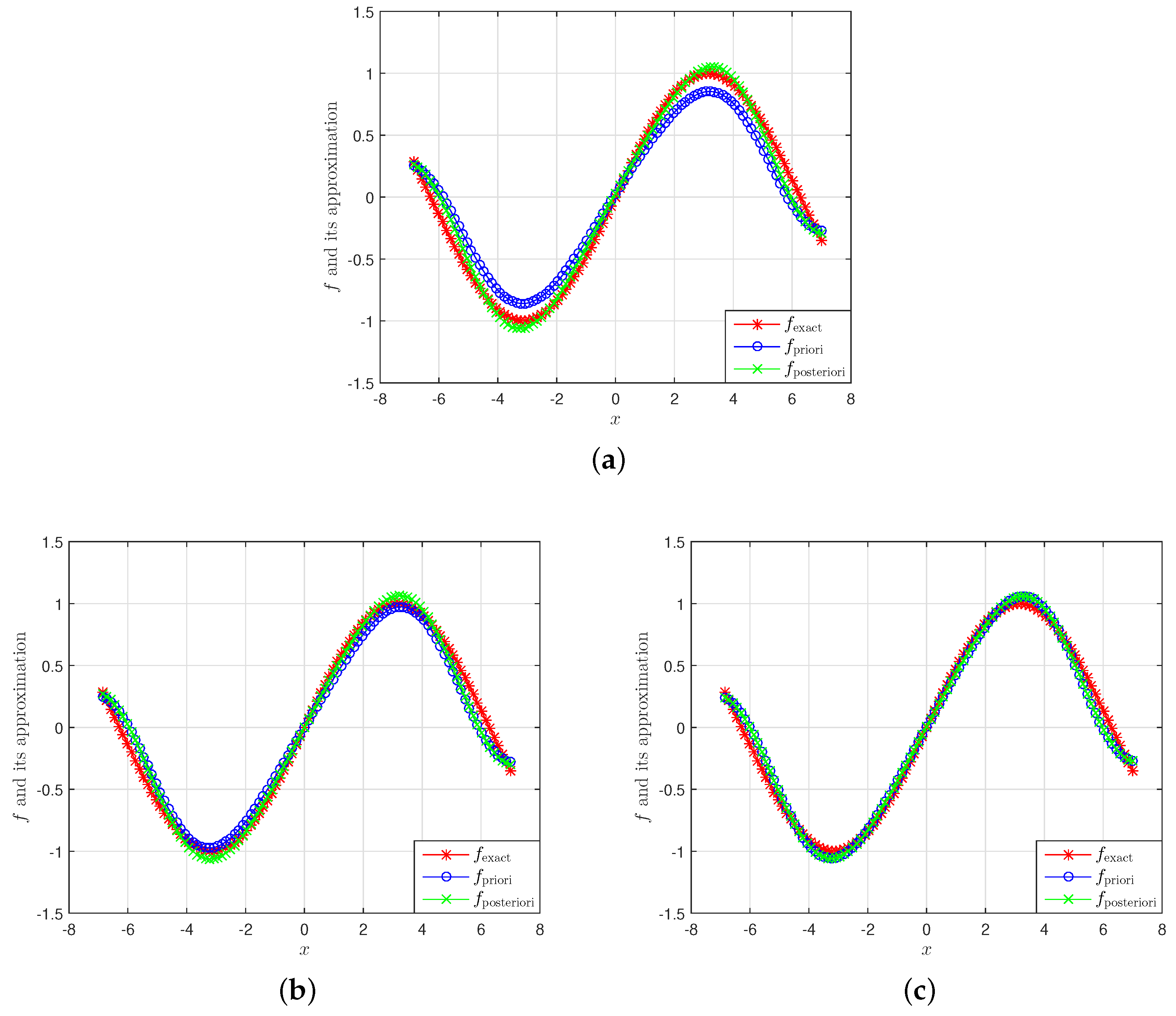
5. Numerical Experiments

In this section, in order to illustrate the usefulness of the proposed methods, we consider the numerical examples intended. We carry out numerically above regularization methods to verify our proposed methods. The numerical examples with $T=1$, and $\beta =0.4$, $\beta =0.95$ are shown in this section, respectively. In the following, we give an example which had the exact expression of the solutions $\left(u\right(x,t),f(x\left)\right)$. We use the computations in Matlab codes which are given by Podlubny [18] for computing the generalized Mittag-Leffler function and the accuracy control in computing is ${10}^{-10}$. We will do the numerical tests with $x\in [-7,7]$ and $\eta =1.1$. The couple of $({\varphi }_{\epsilon },g_{\epsilon })$, which are determined below, play as measured data with a random noise as follows:

$$\begin{array}{c}\hfill {\varphi }_{\epsilon }(·)=\varphi (·)+\epsilon \left(2\mathrm{rand}(.)-1\right),g_{\epsilon }(·)=g(·)+\epsilon \left(2\mathrm{rand}(.)-1\right).\end{array}$$

(71)

Following Reference [9], we know the function $rand(·)$ generates arrays of random numbers whose elements are normally distributed with mean 0, variance ${\sigma }^2=1$ and standard deviation $\sigma =1$, and it gives rand(size(.)) and rand(size(.)) returns an array of random entries that is the same size as g and $\varphi$, respectively. We can easily verify the validity of the inequality:

$$\begin{array}{c}\hfill \parallel {\varphi }_{\epsilon }{-\varphi \parallel }_{C[0,T]}\le \epsilon ,{\parallel g_{\epsilon }-g\parallel }_{{\mathcal{L}}_2\left(\mathbb{R}\right)}\le \epsilon .\end{array}$$

(72)

In this example, we consider particularly a one-dimensional case of the problem (1) for f is an exact data function.

$$\begin{array}{c}\hfill \left\{\begin{array}{c}\frac{{\partial }^{\beta }u(x,t)}{\partial t^{\beta }}=u_{xx}(x,t)+\varphi \left(t\right)f\left(x\right),(x,t)\in \mathbb{R}\times (0,T],\hfill \\ u(x,0)=0,x\in \mathbb{R},\hfill \\ u(x,1)=g\left(x\right),x\in \mathbb{R}·\hfill \end{array}\right.\end{array}$$

(73)

In this example, we choose the following solution

$$u(x,t)=\left(E_{\beta ,1}\left(t^{\beta }\right)-E_{\beta ,1}(-t^{\beta })\right)sin\left(\frac{x}{2}\right).$$

(74)

Then a simple computation yields

$$\varphi \left(t\right)=\frac{5}{4}{E}_{\beta ,1}\left(t^{\beta }\right)+\frac{3}{4}{E}_{\beta ,1}(-t^{\beta }).$$

(75)

and $f\left(x\right)=sin\left(\frac{x}{2}\right)$. Moreover, we have $u(x,0)=u_0\left(x\right)=0$ and

$$\begin{array}{c}\hfill u(x,1)=u_1\left(x\right)=g\left(x\right)=\left(E_{\beta ,1}\left(1\right)-E_{\beta ,1}(-1)\right)sin\left(\frac{x}{2}\right).\end{array}$$

(76)

Next, for computing the integral in the latter equality, see Reference [19], we use the fact that

$$\begin{array}{c}\hfill \underset{0}{\overset{x}{\int }}{u}^{\kappa -1}{E}_{\beta ,\kappa }\left(y{u}^{\beta }\right){(x-u)}^{\beta -1}{E}_{\beta ,\beta }\left(z{(x-u)}^{\beta }\right)du=\frac{y{E}_{\beta ,\kappa +\beta }\left(y{x}^{\beta }\right)-z{E}_{\beta ,\beta +\kappa }\left(z{x}^{\beta }\right)}{y-z}{x}^{\beta +\kappa +1}·\end{array}$$

(77)

From ${\varphi }_{\epsilon }(.)=\varphi (.)+\epsilon \left(2\mathrm{rand}(.)-1\right)$, we have

$$\begin{array}{cc}\hfill \underset{0}{\overset{1}{\int }}{s}^{\beta -1}{E}_{\beta ,\beta }(-{\xi }^2{s}^{\beta }){\varphi }_{\epsilon }(1-s)ds& =\underset{0}{\overset{1}{\int }}{s}^{\beta -1}{E}_{\beta ,\beta }(-{\xi }^2{s}^{\beta })\varphi (1-s)ds\hfill \\ \hfill & +\epsilon \left(2\mathrm{rand}(.)-1\right)\underset{0}{\overset{1}{\int }}{s}^{\beta -1}{E}_{\beta ,\beta }(-{\xi }^2{s}^{\beta })ds·\hfill \end{array}$$

(78)

Combining (72), (75) and (78), we have

$$\begin{array}{cc}\hfill \underset{0}{\overset{1}{\int }}{s}^{\beta -1}{E}_{\beta ,\beta }(-{\xi }^2{s}^{\beta -1}){\varphi }_{\epsilon }(1-s)ds=& \frac{5}{4}\left(\frac{E_{\beta ,\beta +1}\left(1\right)+{\xi }^2{E}_{\beta ,\beta +1}(-{\xi }^2)}{1+{\xi }^2}\right)\hfill \\ & -\frac{3}{4}\left(\frac{E_{\beta ,\beta +1}(-1)-{\xi }^2{E}_{\beta ,\beta +1}(-{\xi }^2)}{-1+{\xi }^2}\right)\hfill \\ & +\frac{\epsilon \left(2\mathrm{rand}(.)-1\right)}{{\xi }^2}\left(1-E_{\beta ,1}(-{\xi }^2)\right).\hfill \end{array}$$

(79)

In general, the numerical methods referenced by References [20,21] are summarized in three steps as follows.

Step 1: Choose N to generate the spatial and temporal discretization in such a manner as:

$$\begin{array}{c}\hfill x_i=i\Delta x,\Delta x=\frac{\pi }{N},i=\overline{0,N}.\end{array}$$

(80)

Obviously, the higher value of N will provide numerical results that are more accurate and stable. Here we choose $N=100$ is satisfied.

Step 2: Setting $f_{\epsilon ,\alpha }\left(x_i\right)=f_{\epsilon ,\alpha }^i$ and $f\left(x_i\right)=f^i$, constructing two vectors contained all discrete values of $f_{\epsilon ,\alpha }$ and f denoted by ${\Lambda }_{\epsilon ,\alpha }$ and $\Psi$, respectively.

$$\begin{array}{cc}\hfill & {\Lambda }_{\epsilon ,\alpha }=[f_{\epsilon ,\alpha }^0{f}_{\epsilon ,\alpha }^1...f_{\epsilon ,\alpha }^Q]\in {\mathbb{R}}^{Q+1},\hfill \\ \hfill & \Psi =[f^0{f}^1...f^{Q-1}{f}^Q]\in {\mathbb{R}}^{Q+1}·\hfill \end{array}$$

(81)

Step 3: The estimation is defined:

Relative error estimation:

$$\begin{array}{c}\hfill E_1=\frac{\sqrt{{\displaystyle \sum _{i=1}^N}{|f_{\epsilon ,\alpha }\left(x_i\right)-f\left(x_i\right)|}_{{\mathcal{L}}_2(-7,7)}^2}}{\sqrt{{\displaystyle \sum _{i=1}^N}{\left|f\left(x_i\right)\right|}_{{\mathcal{L}}_2(-7,7)}^2}}·\end{array}$$

(82)

Absolute error estimation:

$$\begin{array}{c}\hfill E_2=\sqrt{\frac{1}{N}\sum _{i=1}^N{|f_{\epsilon ,\alpha }\left(x_i\right)-f\left(x_i\right)|}_{{\mathcal{L}}_2(-7,7)}^2}·\end{array}$$

(83)

Figure 1 shows a 2D figures between the sought and its regularized solutions for $N=100$ and $\beta =0.95$. All figures are presented with $\epsilon =0.1$, $\epsilon =0.01$ and $\epsilon =0.001$, respectively.

In

Table 1. The error estimation between the exact and regularized solutions of this example at $\beta =0.95$ with $N=100$.

$\mathit{\epsilon }$	${\mathit{E}}_1^{{\mathit{\beta }}_{\mathit{pri}}}$	${\mathit{E}}_1^{{\mathit{\beta }}_{\mathit{pos}}}$	${\mathit{E}}_2^{{\mathit{\beta }}_{\mathit{pri}}}$	${\mathit{E}}_2^{{\mathit{\beta }}_{\mathit{pos}}}$
0.1	0.279660141830880	0.163452531664322	0.188256991900635	0.110030273632189
0.01	0.167130513450332	0.146077554813055	0.112506156619184	0.098334073898654
0.001	0.144054212078375	0.144599158066180	0.096972033479447	0.097338871212350

and

Table 2. The error estimation between the exact and regularized solutions with the different values of $\beta$, $\epsilon =0.01$ and $N=100$.

$\mathit{\beta }$	${\mathit{E}}_1^{{\mathit{\beta }}_{\mathit{pri}}}$	${\mathit{E}}_1^{{\mathit{\beta }}_{\mathit{pos}}}$	${\mathit{E}}_2^{{\mathit{\beta }}_{\mathit{pri}}}$	${\mathit{E}}_2^{{\mathit{\beta }}_{\mathit{pos}}}$
0.2	0.156401672575436	0.176079016470940	0.078962919638416	0.092189970426402
0.4	0.146364358305196	0.165153671589525	0.073895354649786	0.086469770247512
0.6	0.136338164832119	0.153413164488168	0.068833404246973	0.080322774289912
0.8	0.124692172130227	0.140316883268202	0.062953661590221	0.073465933522836

of this example, we show the error estimation both the priori and the posteriori within case $N=100$, that is, in Table 1 we show the error estimation for both the priori and the posteriori at $\beta =0.95$ with $\epsilon \in \{0.1,0.01,0.001\}$, respectively. In Table 2, we show the relative error estimation and absolute error estimation both the priori and the posteriori with $\epsilon =0.01$ with the different values of $\beta \in \{0.2,0.4,0.6,0.8\}$, when $\epsilon$ is fixed and the mesh resolutions are increased, the regularized solution convergence is better than that of the exact solution. From observing the results from the tables and figures above, we conclude that when $\epsilon$ tends to zero, the regularized solution approaches the exact solution.

6. Conclusions

In this study, by using the mollification regularization method, we solved the inverse problem and recovered the source term for time fractional diffusion equation with the time dependent coefficient. In the theoretical results, which we have shown, we obtained the error estimates of both a priori and a posteriori parameter choice rule methods based on a priori condition. In addition, in the numerical results, it shows that the regularized solutions are converged to the exact solution. Furthermore, it also shows that the smaller error of the input data, the better the convergence results.

References

1. Malyshev, I. An inverse source problem for heat equation. J. Math. Anal. Appl. 1989, 142, 206–218. [Google Scholar] [CrossRef] [Green Version]
2. Geng, F.; Lin, Y. Application of the variational iteration method to inverse heat source problems. Comput. Math. Appl. 2009, 58, 2098–2102. [Google Scholar] [CrossRef] [Green Version]
3. Shidfar, A.; Babaei, A.; Molabahrami, A. Solving the inverse problem of identifying an unknown source term in a parabolic equation. Comput. Math. Appl. 2010, 60, 1209–1213. [Google Scholar] [CrossRef] [Green Version]
4. Barkai, E.; Metzler, R.; Klafter, J. From continuous time random walks to the fractional Fokker-Planck equation. Phys. Rev. E 2000, 61, 132–138. [Google Scholar] [CrossRef] [PubMed]
5. Chaves, A. Fractional diffusion equation to describe Levy flights. Phys. Lett. A 1998, 239, 13–16. [Google Scholar] [CrossRef]
6. Gorenflo, R.; Mainardi, F.; Scalas, E.; Raberto, M. Fractional calculus and continuoustime finance, the diffusion limit. In Mathematical Finance. Trends in Mathematics; Birkhuser: Basel, Switzerland, 2001; pp. 171–180. [Google Scholar]
7. Sakamoto, K.; Yamamoto, M. Initial value/boundary value problems for fractional diffusion-wave equations and applications to some inverse problems. J. Math. Anal. Appl. 2011, 382, 426–447. [Google Scholar] [CrossRef] [Green Version]
8. Zhang, Z.Q.; Wei, T. Identifying an unknown source in time-fractional diffusion equation by a truncation method. Appl. Math. Comput. 2013, 219, 5972–5983. [Google Scholar] [CrossRef]
9. Yang, F.; Fu, C.L. The quasi-reversibility regularization method for identifying the unknown source for time fractional diffusion equation. Appl. Math. Modell. 2015, 39, 1500–1512. [Google Scholar] [CrossRef]
10. Wei, T.; Wang, J.G. A modified Quasi-Boundary Value method for an inverse source problem of the time fractional diffusion equation. Appl. Numer. Math. 2014, 78, 95–111. [Google Scholar] [CrossRef]
11. Yang, F.; Fu, C.L.; Li, X.X. A mollification regularization method for identifying the time-dependent heat source problem. J. Engine Math. 2016, 100, 67–80. [Google Scholar] [CrossRef]
12. Wei, T.; Wang, J.G. Quasi-reversibility method to identify a space-dependent source for the time-fractional diffusion equation. Appl. Math. Modell. 2015, 39, 6139–6149. [Google Scholar] [CrossRef]
13. Nguyen, H.T.; Le, D.L.; Nguyen, V.T. Regularized solution of an inverse source problem for the time fractional diffusion equation. Appl. Math. Modell. 2016, 40, 8244–8264. [Google Scholar] [CrossRef]
14. Podlubny, I. Fractional Differential Equations; Academic Press: San Diego, CA, USA, 1999. [Google Scholar]
15. Samko, S.G.; Kilbas, A.A.; Marichev, O.I. Fractional Integrals and Derivatives: Theory and Application; Gordon and Breach: New York, NY, USA, 1993. [Google Scholar]
16. Yang, F.; Fu, C.L. A mollification regularization method for the inverse spatial-dependent heat source problem. J. Comput. Appl. Math. 2014, 255, 555–567. [Google Scholar] [CrossRef]
17. Kirsch, A. An Introduction to the Mathematical Theory of Inverse Problem; Applied Mathematical Sciences; Springer Science Business Media: Berlin/Heidelberg, Germany, 2011. [Google Scholar]
18. Podlubny, I.; Kacenak, M. Mittag-Leffler Function. The MATLAB Routine. 2006. Available online: http://www.mathworks.com/matlabcentral/fileexchange (accessed on 19 September 2019).
19. Mathai, A.M.; Haubold, H.J. Mittag Leffler function and Fractional Calculus. In Special Functions for Applied Scientists; Springer: New York, NY, USA, 2008; Chapter 2. [Google Scholar]
20. Meerschaert, M.; Tadjeran, C. Finite difference approximations for two-sided spacefractional partial differential equations. Appl. Numer. Math. 2006, 56, 80–90. [Google Scholar] [CrossRef]
21. Bu, W.; Liu, X.; Tang, Y.; Jiang, Y. Finite element multigrid method for multiterm time fractional advection-diffusion equations. Int. J. Model. Simul. Sci. Comput. 2015, 6, 1540001. [Google Scholar] [CrossRef]
Figure 1. A comparison between the exact and regularized solutions for k = 1 , β = 0.95 with N = 100 . (a) ε = 0.1 . (b) ε = 0.01 . (c) ε = 0.001 .
Mathematics 07 01048 g001