Comparing Direct and Indirect Transmission in a Simple Model of Veterinary Disease

Abstract

Foodborne diseases are a longstanding worldwide public health concern. Modeling the transmission pathways of foodborne pathogens accurately and effectively can aid in understanding the spread of pathogens and facilitate decision making for intervention. A new compartmental model is reported that integrates the effects of both direct and indirect transmission. Depending on the choice of epidemiological parameters, the model can be tuned to be purely direct, purely indirect, or used to explore the dynamics in an intermediate regime. Steady state analysis of the model and limiting cases are studied. A numerical simulation is employed to study the impact of different epidemiological parameters and dose response. Direct transmission can surpass the effect of indirect transmission for the same range of parameter values and result in an earlier epidemic. The rate at which the pathogens are removed from the environment can lead to a faster epidemic. The environmental contamination can decrease the time to reach the steady state depending on the dose response. These results can inform policy makers for control strategies to reduce foodborne pathogen transmission.

1. Introduction

Foodborne diseases have become a growing concern in public health globally. In the US, one in every six persons is affected by foodborne disease every year [1]. In the European Union, over 320,000 cases are reported each year [2]. The protection from food-borne zoonoses starts at the farm level. Understanding the transmission of foodborne zoonoses can aid in analysis, assessing risks, and making recommendations for public health officials. Mathematical models can identify intervention strategies and enhance the decision-making process by providing scientific understanding of the spread of the pathogens and their control.

Transmission is a key element that constitutes the basis of the mathematical model. Transmission can be captured by the identification of states. Thus, selection of states to represent the epidemiology of the disease is crucial. There are models that include infectious transient shedder, latent infectious, infectious low shedder, infectious high shedder, clinically infectious, sub-clinically infectious, and carrier states to cover different levels of transmission [3,4,5]. Adding more states increases the complexity of the model by requiring accurate estimate of additional epidemiological parameters. Thus, simple models that capture the general transmission dynamics with few states can be valuable for decision making, provided the simple model does not obscure important aspects of transmission.

Two important possible channels of transmission for foodborne disease have been well studied. Foodborne pathogens can be directly transmitted from animal to animal (fecal-oral infections, infections spread through direct contact) or indirectly via free-living bacteria present in the environment (indirect contact) [3]. A Susceptible-Infected (S-I) model for direct transmission assumes the transmission can be described as animal to animal. In poultry flocks, for example, if susceptible birds immediately consume contaminated feces from infectious birds, an S-I contact model may be appropriate. However, transmission of some foodborne pathogens such as Campylobacter may require explicitly modeling of the accumulation of contaminated waste. Transmission of Campylobacter can occur indirectly through contaminated feces, contaminated water, or other environmental pathways [6]. If the environmental contamination builds up over time, or if the rate of transmission depends on a dose-response effect, then a simple S-I model may be inadequate.

Van Gerwe et al. [7] illustrate the direct contact transmission rate of Campylobacter among broilers. Environmental transmission can be represented by fecal shedding to the internal environment within a farm, followed by ingestion. Lurette et al. [4] give an example of indirect contact-based transmission, with models of the spread of Salmonella in pig production where the main route of the transmission is indirect transmission via free-living Salmonella in the pen. As environmental sources of infection build up, the probability of transmission may be nonlinear. Risk assessment of foodborne zoonoses and dose-response relationships of pathogens have been studied. The effects of age, colonization, and different treatment methodologies have been investigated [8,9]. A systematic analysis of environmental contamination seems to be missing and would be valuable, suggesting the need for further controlled experiments.

It is important to understand the relative importance of direct vs. indirect transmission, and to understand which (if either) dominates for different organisms as a function of farming practice. This understanding could advise intervention strategies, provide insight into sensitive steps in the production process that place animals under stress, and possibly suggest improvements to factory farming protocols.

Finally, depending on the time of animal harvest, infection in animal populations might not reach steady state. In this case, analytic steady state solution of mathematical models will not capture the infection dynamics at time of harvest and numerical solutions can be of great value.

This paper focuses on poultry diseases. The farming protocols for poultry production are highly variable when compared to corresponding protocols for beef and pork. Poultry production depends on both local practice and on the end product of the poultry. The time to raise poultry varies from 3 weeks (for poussins) to 15 months (for heavy hens) with an average of 6–7 weeks [10,11]. The production system varies from country to country. While the US and Russia are focused on integrated poultry production systems that allow them to control feed, rearing, and processing, Europe still has less integrated systems [12]. Thinning, that is, partial depopulation in the broiler house, is widespread in Europe. However it is rare in the US [13]. Thinning has been shown to increase the risk of foodborne disease [13,14]. Additionally, timing of thinning has been addressed for one of the factors in the pathogen status at slaughter [15]. Differences in the rearing practices (all in/all out vs. multiple batch system) are also another factor for foodborne disease [12,16].

Models studying veterinary diseases mostly focus on understanding the transmission rates and the population wide impacts of interventions. Van Wagenberg et al. [17], Doerr et al. [18], Conlan et al. [12], Van Gerwe et al. [19], and Ross [20] are valuable examples of this in modeling foodborne pathogens. Cousins et al. [21] and Liao et al. [22] study the human disease transmission of zoonotic diseases. Rushton et al. [23] analyze the risk factors for Campylobacter transmission. Sibanda et al. [24] provide a good overview of the farm practices on Campylobacter management. These studies focus on mainly one type of transmission.

In this paper, we propose a general framework that captures any combination of direct and indirect transmission of foodborne diseases at the farm level. A compartmental model with three states is employed. We discuss the steady state solution to this general framework along with its limiting cases. We also show how the model can be generalized to capture the effects of dose response. A numerical simulation is developed to study the population dynamics at the time of harvest and to conduct sensitivity analysis on the epidemiological parameters. The numerical solution is found deterministically, although the implementation also supports use of a stochastic solver. We propose that this framework, combined with future controlled experiments, can help identify where particular production facilities operate in the space of contact vs. indirect transmission, which description is most appropriate for different micro parasitic infections, and what intervention strategies may be most effective.

2. Materials and Methods

2.1. Extension of S-I Model

An extension of the S-I model is developed to include environmental contamination in addition to direct transmission. Once an animal is contaminated by the pathogen, there is no recovery from the pathogen. The population size is assumed to be constant over the time horizon. Figure 1 gives the graphical representation of the model, where:

• $N$ is the population size;
• S and I represent the number of susceptible and infected animals in the system so that $N=S+I;$
• $Q$ describes the amount of infectious environmental contamination (e.g., animal waste or contaminated water);
• $\beta$ represents the rate of direct contact-based transmission;
• $ϵ$ represents the rate at which new infections are produced via contaminated agents in the environment (Q);
• $\alpha$ is the rate at which infectious individuals create new contaminated agents (Q); and
• $k$ is the rate at which the environment is cleared of waste (by dissipation or active cleaning).

The following ordinary differential equations summarize the model:

$$\begin{gathered} \frac{dS}{dt}=-\beta \frac{SI}{N}-ϵ\frac{SQ}{N}+\mu I \\ \frac{dI}{dt}=-\frac{dS}{dt}=\beta \frac{SI}{N}+ϵ\frac{SQ}{N}-\mu I \\ \frac{dQ}{dt}=-kQ+\alpha I \end{gathered}$$

(1)

The mass action term $\beta \frac{SI}{N}$ is the new incidence of infections caused by contact-based infection, while the term $ϵ\frac{SQ}{N}$ describes new infections resulting from exposure to the contaminated environmental agents. The rate of change in the susceptible and the infectious population are the same except for their sign. The first term in the environment rate change accounts for the removal from the environment, while the last term in this equation defines the rate at which environmental contamination is created by infectious individuals.

We note that Equation (1) defines frequency dependent transmission. One could adopt a density dependent form where the mass action term would be written as $\beta SI$, which can be valuable for some veterinary diseases. Note that since $\beta$ and $N$ are constants, we could combine them as a new parameter ${\beta }^{\prime }\equiv \beta /N$, and express our results as density dependent rather than frequency dependent (simply rescaling the constant).

The differential Equation (1) is most appropriate as a model of continuous production or where flocks (or herds) are thinned at a characteristic rate, $\mu$. In particular we note that $\mu$ does not represent a mortality rate but rather sets the natural timescale of production. For all in/all out production, the same equations can be used with initial state $I=0$, and final state determined by integrating the equations to the time of final harvest or slaughter. The current model does not include a recovered state because it is assumes that animals do not recover on the production timescales. However, for pathogens where recovery is possible, it can be easily added as an extension to this model.

2.2. Analysis in Steady State, Analytic Solution

In steady state, there would be no change in the infected number of animals and the amount of environmental contamination, so that the derivatives of these quantities are zero:

dI/dt = 0,dQ/dt = 0

Thus, the following is obtained for the environmental contamination term from the third differential equation above:

$$Q^{\ast }=\frac{\alpha }{k}{I}^{\ast }$$

(2)

By substituting $S=N-I$ and inserting Equation (2) into the second differential equation above:

$$0=\left[\beta -\frac{ϵ\alpha }{Nk}{I}^{\ast }-\mu \right]I^{\ast }-\frac{\beta }{N}{I}^{{\ast }^2}+\frac{ϵ\alpha }{k}{I}^{\ast }$$

(3)

Here $I^{\ast }$ = 0 is a trivial solution to Equation (3).

For $I^{\ast }\ne 0$, dividing Equation (3) by $I^{\ast }$ yields:

$$\frac{I^{\ast }}{N}\left[\beta +\frac{ϵ\alpha }{k}\right]=\beta +\frac{ϵ\alpha }{k}-\mu$$

(4)

Rearranging the terms in Equation (4), an expression of prevalence is obtained in terms of a reproductive number R₀:

$$\frac{I^{\ast }}{N}=\frac{\beta +\frac{ϵ\alpha }{k}-\mu }{\beta +\frac{ϵ\alpha }{k}}=1-\frac{\mu }{\beta +\frac{ϵ\alpha }{k}}=1-\frac{1}{R_0}$$

where

$$R_0=\frac{\beta +\frac{ϵ\alpha }{k}}{\mu }.$$

(5)

To get a better sense of the behavior of these quantities, we consider how $Q$ behaves when $\frac{dI}{dt}$ = 0 (the definition of steady state), and how $I$ behaves when $\frac{dQ}{dt}=0.$ The relations obtained hold approximately when these conditions hold approximately, that is, when $\frac{dI}{dt}$ is very small but not zero, and similarly for $\frac{dQ}{dt}$.

When $\frac{dI}{dt}$ = 0, but $\frac{dQ}{dt}$ is not held to zero, then

$$Q_1=C{e}^{-kt}+\frac{\alpha }{k}I$$

is a solution for $Q$, where $C$ is an arbitrary constant, since:

$$\frac{d{Q}_1}{dt}=C\left(-k\right)e^{-kt}= -k{Q}_1+\alpha I$$

If we assume $\frac{dQ}{dt}=0$, so that $Q_1=\frac{\alpha }{k}I$ is a solution for $Q$, then we have:

$$\frac{dI}{dt}=\beta \frac{SI}{N}+ϵ\frac{\frac{S\alpha I}{k}}{N}-\mu I=\frac{SI}{N}\left(\beta +\frac{ϵ\alpha }{k}\right)-\mu I$$

That is,

$$\frac{dI}{dt}\approx \frac{SI}{N}\mu R_o-\mu I=\mu I\left(R_{eff}-1\right)$$

(6)

with $R_{eff}\equiv \frac{S}{N}{R}_0$ when $\frac{dQ}{dt}=0$.

We note also that in general

$$Q_2=C{e}^{-kt}+\frac{\alpha }{k}(I-\frac{I^{\prime }}{k}+\frac{I^{″}}{k^2}-\frac{I^{‴}}{k^3}\dots )$$

(7)

is a solution for $Q$. Here $I^{\prime }=\frac{dI}{dt}, I^{″}=\frac{d^{2}I}{d{t}^2},$ and so on. This is readily verified by substituting into

$$\frac{dQ}{dt}=-kQ+\alpha I$$

2.3. Limiting Cases Outside Steady State

In this section, we study the limiting cases to understand the disease state analytically outside steady state. Although $I^{\prime }=\frac{dI}{dt}$ probably is not exactly maximum at $I=S=N/2,$ the contribution of $\beta SI/N$ to $I^{\prime }$ is maximized under that condition, and approximating $Q$ under the assumption that $I^{\prime }=0$ is likely to fail at $I=S=N/2$. However, if $I^{\prime }$ is nearly maximum, then $I^{″}$ is nearly zero, so it is informative to explore the solution under the assumption that $I^{″}$ is small, making the approximation $Q\approx \frac{\alpha }{k}I-\frac{\alpha }{k^2}{I}^{\prime }$ plausible, via truncation of Equation (7) and choosing $C=0$. This is not a substitute for a numerical solution of the true dynamics, but is a simplification that allows us to estimate the disease state away from steady state and where the rate of epidemic growth is maximal. Assuming $I^{″}$ is small, so that $Q\approx \frac{\alpha }{k}I-\frac{\alpha }{k^2}{I}^{\prime }$, then $I^{\prime }=\frac{\beta SI}{N}+\frac{ϵSQ}{N}-\mu I \approx \frac{\beta SI}{N}+\frac{ϵS}{N}\left(\frac{\alpha }{k}I-\frac{\alpha }{k^2}{I}^{\prime }\right)-\mu I$ and so, adding $\frac{Sϵ\alpha }{N{k}^2}{I}^{\prime }$ to both sides and dividing:

$$I^{\prime }\approx \frac{\frac{SI}{N}\mu R_0-\mu I}{\left(1+\frac{Sϵ\alpha }{N{k}^2}\right)} =\frac{\mu I\left(R_{eff}-1\right)}{\left(1+\frac{Sϵ\alpha }{N{k}^2}\right)}$$

(8)

That is, up to the scaling by $\frac{1}{1+\frac{Sϵ\alpha }{N{k}^2}},$ the equation for $I^{\prime }=dI/dt$ when $I^{\prime }$ is maximal (or more generally, at a critical point) is the same as when $\frac{dQ}{dt}$ is zero, and the scaling is close to 1 when $S=I=N/2$ and $k$ is large, so that $\frac{Sϵ\alpha }{N{k}^2}=\frac{ϵ\alpha }{2k^2}\ll 1$.

2.4. Modeling Dose Response

Infection rates for some foodborne pathogens like Campylobacter have also been studied in terms of a dose-response model [25]. A dose-response or exposure-response model is appropriate when the transmission rate varies based changing levels of exposure (or dose). Dose-response effects for direct transmission have been developed using a nonlinear mass action term of the form ${\beta }^{\prime }\frac{S}{N}{\left(I\right)}^p$ [26]. With an exponent with p > 1, transmission is attenuated for small I and amplified for large I (the threshold infectious concentration is a constant absorbed in ${\beta }^{\prime }$).

It is straightforward to extend this nonlinear dose-response expression for indirect transmission. The contact infection term becomes $ϵ\frac{S}{N}{\left(\frac{Q}{Q_0}\right)}^{\nu }.$ Determining a specific value for $\nu$ requires new experimental data, but it is possible to derive the steady state behavior in closed form.

With this dose-response model, the first and second differential equations become:

$$\begin{gathered} \frac{dS}{dt}=-\beta \frac{SI}{N}-ϵ\frac{S}{N}{\left(\frac{Q}{Q_0}\right)}^{\nu }+\mu I \\ \frac{dI}{dt}=\beta \frac{SI}{N}+ϵ\frac{S}{N}{\left(\frac{Q}{Q_0}\right)}^{\nu }-\mu I \end{gathered}$$

(9)

where $\nu >1$ and $Q_0$ is the threshold dose for the environmental contamination. With exponent $\nu >1,$ the rate of infection is attenuated for low Q and amplified at high Q. By dimensional analysis we expect:

$$R_{eff}~\frac{\beta +\frac{ϵ}{Q_o^{\nu }}{\left(\frac{\alpha }{k}\right)}^{\nu }}{\mu }$$

(10)

For $\nu =1$, Equation (9) reduces to Equation (1). The critical dose, Q₀, is a constant that rescales $ϵ$. Combining constants, one could define:

$${ϵ}^{\prime }=ϵ{\left(\frac{1}{Q_0}\right)}^{\nu }$$

(11)

Low critical dose (and high $\nu$) serves to amplify the rate of infection from environmental contamination at long times.

General values of $\nu$ require a numerical solution. For $\nu =2$, we can solve for the steady state $I_2^{\ast }$ by setting $\frac{dI}{dt} and \frac{dQ}{dt}$ to zero, via Equation (9) for $I$ and Equation (1) for $Q$. From Equation (1), we have $Q=\left(\frac{\alpha }{k}\right)I$, and from Equation (9), and substituting $S=N-I$, we have $\beta \frac{\left(N-I\right)I}{N}+ϵ\frac{N-I}{N}{\left(\frac{\left(\frac{\alpha }{k}\right)I}{Q_0}\right)}^2-\mu I=0$.

Dividing out an $I$ factor, and setting $z\equiv 1-\frac{I}{N}$ and $\gamma \equiv ϵ{\left(\frac{\left(\frac{\alpha }{k}\right)}{Q_0}\right)}^2$, after dividing through by $N,$ we have $\frac{\beta }{N}z+\gamma z\left(1-z\right)-\mu \left(1-z\right)=0$.

That is,

$$\gamma z^2-\left(\frac{\beta }{N}+\gamma +\mu \right)z+\mu =0$$

So that in steady state the endemic level of infection becomes:

$$I_2^{\ast }= N\left(1-\frac{\frac{\beta }{N}+\gamma +\mu \pm \sqrt{{\left(\frac{\beta }{N}+\gamma +\mu \right)}^2-4\gamma \mu }}{2\gamma }\right).$$

We will not attempt any further simplification, but observe that this closed-form expression is readily computable.

2.5. Numerical Simulation

The deterministic numerical solution described here was first implemented and tested in MATLAB. The results reported come from the original implementation. The same algorithm was then re-implemented in Java and made available as open source through the Eclipse Foundations Spatio Temporal Epidemiological Modeler project [27] so the source code is open and available to all. The implementation in STEM allows the same model to be run either deterministically or stochastically. To study the system dynamics, the ordinary differential equations were integrated using a variable step Runge–Kutta Method. Different sensitivity analyses are employed to investigate the infections in steady state and at the time of harvest, as well as to investigate the effect of important epidemiological parameters. From Equation (5) we note that there are two primary contributors to the reproductive number:

$$R_0=R_{direct}+R_{indirect}$$

For direct contact, $R_{direct}=\raisebox{1ex}{$\beta $}\!\left/ \!\raisebox{-1ex}{$\mu $}\right.$, as for any basic SI model. For indirect contact, $R_{indirect}=\frac{ϵ\alpha }{\mu k}$. Accordingly, we chose epidemiological parameters to explore reproductive numbers in the range of $0<R_0<3.6,$ with equal contributions from both direct and indirect transmission. The values and ranges used are shown in

Table 1. Epidemiological parameters were chosen to explore a range of reproductive number with equivalent contribution possible from direct and/or indirect transmission. The epidemiological parameters are known to vary with strain [9], but the range of values listed in the table are based on typical values from the literature [6,7,8,13,17].

Parameter	Value of Range [a,b]	Contribution to Reproductive Number	Range [a,b]
$\alpha$ [day−1]	0.1	$R_{indirect}=\frac{ϵ\alpha }{\mu k}$	[0,3.6]
$ϵ$ [day−1]	[0,0.12]
$k$ [day−1]	0.1 [17]	$R_{direct}=\raisebox{1ex}{$\beta $}\!\left/ \!\raisebox{-1ex}{$\mu $}\right.$	[0,3.6]
$\beta$ [day−1]	[0,0.12] [7]
$\mu$ [day−1]	1/30 [13]	-
N	1

. Later we will also study the sensitivity of $R_{indirect}$ to relative variations in $\alpha , ϵ, \mathrm{and} k.$ For the purposes of this simulation, we consider the timescales characteristic of poultry production where flocks may be harvested in less than 90 days.

3. Results

In this section, we present the results of the numerical simulation. In Figure 2, we compare the analytic steady state solution obtained in Section 2 with the numerical simulation at long time (t = 1000 days). The figure is a heat map of the fraction of infectious animals as a function of $R_{direct}=\raisebox{1ex}{$\beta $}\!\left/ \!\raisebox{-1ex}{$\mu $}\right.$, and $R_{indirect}=\frac{ϵ\alpha }{\mu k}$ with epidemiological parameters listed in Table 1. At long time, the numerical simulation agrees well with the expected steady state behavior. For $R_0<1,$ there is no epidemic ($I=0$ shown in blue), with a sharp transition to $I=1$ (red) for $R_0>1$. We observe that the effects of the contact-based infection and the environment-based infection at long times are equivalent.

However, as discussed above, portions of a poultry flock may be selected for slaughter in as little as 30 days with full “harvest” in less than 100 days. On this timescale the epidemic curve may still be far from steady state. Figure 3a shows a heat map of the fraction of infectious animals as a function of $R_{direct}=\raisebox{1ex}{$\beta $}\!\left/ \!\raisebox{-1ex}{$\mu $}\right.$, $R_{indirect}=\frac{ϵ\alpha }{\mu k}$, at t = 100 days using the same epidemiological parameters. The same data is presented as a 3D surface plot in Figure 3b. The fact that the system is far from steady state is evidenced by both the broad transition region and the fact that the epidemic is observed for higher values of $R_0$ at short time. The transition is no longer symmetric in $R_{direct}$ and $R_{indirect}.$ Saturation of the infectious population is observed for $R_{direct} >\sim 2.0$, whereas the infraction for infectious production system dominated by indirect transmission would not exhibit saturation until $R_{indirect} >\sim 3.0$ with the parameters shown in Table 1. This figure can be used to understand the impact of thinning practices in the farms by changing the parameters of use.

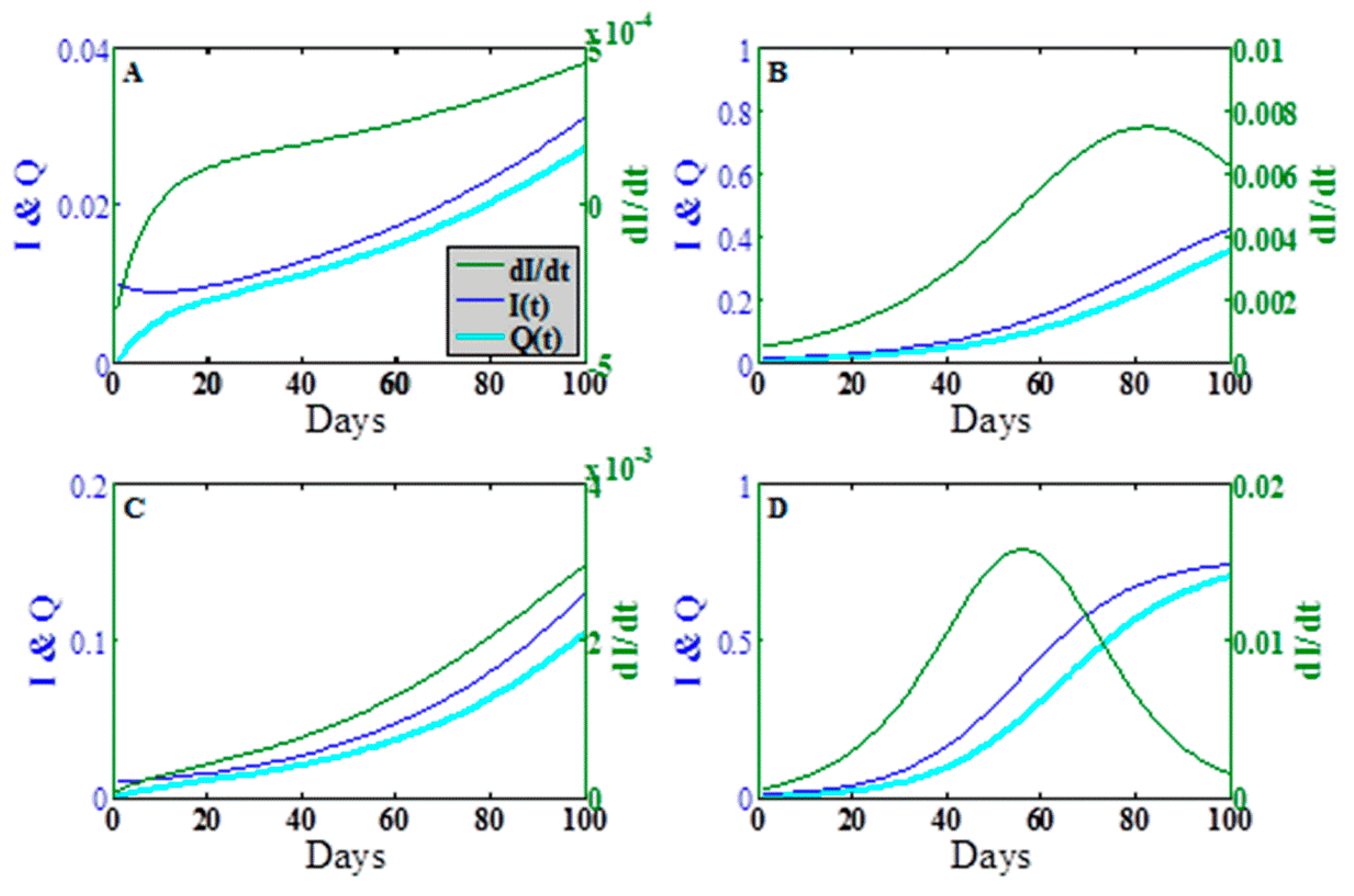
To explore the dynamic behavior in greater detail, we plot in Figure 4 the epidemic wave for the fraction infectious $I\left(t\right),$ the concentration $Q\left(t\right),$ and the rate of change $dI/dt$ in the time period $0\le t\le 100$ days at the points designated A, B, C, D in Figure 3a. Points A, B, and C show the early onset of the epidemic wave contact dominated transmission, indirect transmission limit, and mixed transmission modes, respectively. Point D shows the full epidemic wave for $R_{direct} \mathrm{and} R_{indirect}$, both large.

The asymmetry of the transition in Figure 4a,b indicates that the approach of the dynamics to steady state for direct vs. indirect transmission can vary dramatically, especially over the short time scales characteristic of food production. 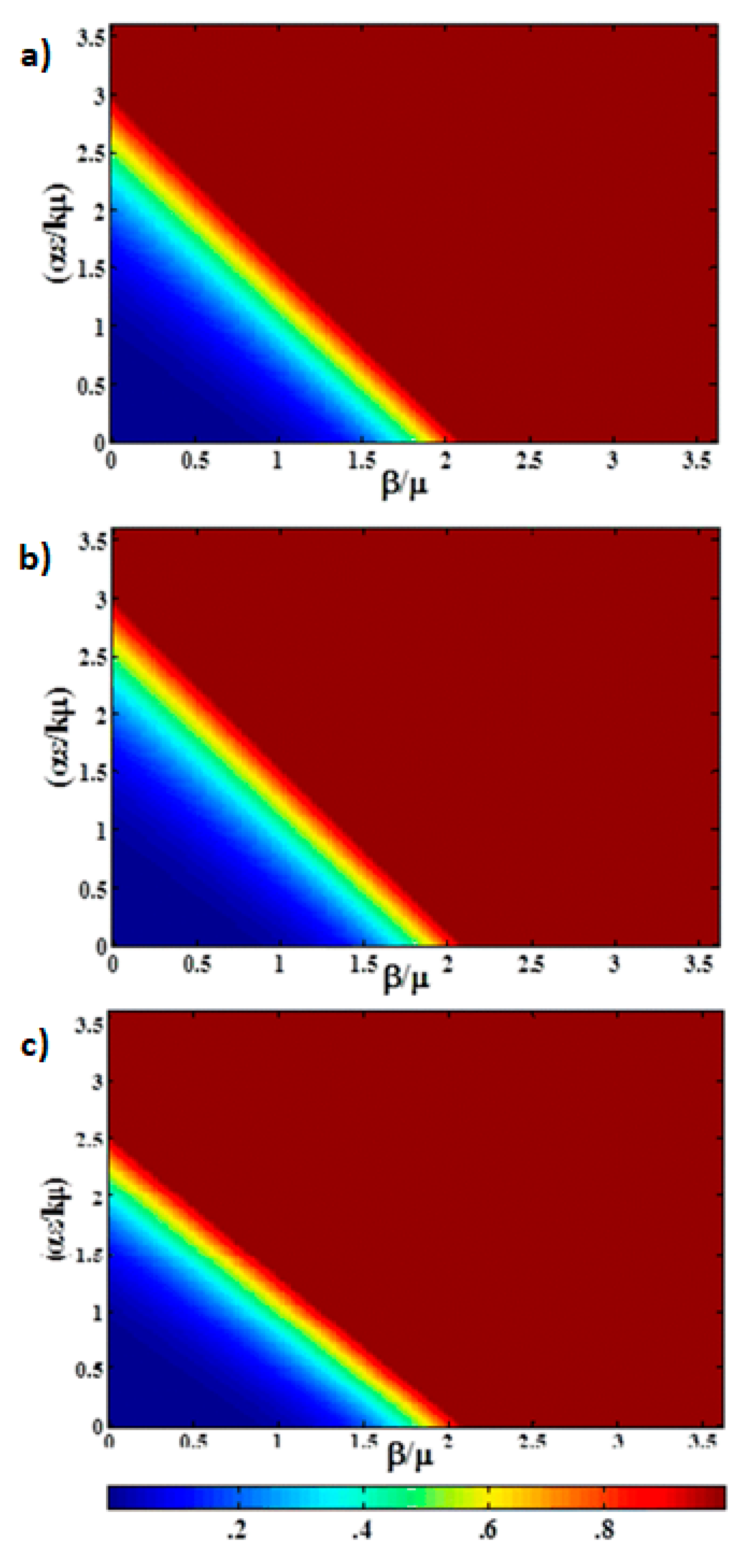Furthermore, the epidemic time scales for indirect transmission depend not only on the intrinsic epidemiological parameters $ϵ,\alpha , \mathrm{and} \mu$, but also on the clearing or cleaning rate k which may vary with production practices. Thus, we next study the sensitivity analysis for various parameters. In Figure 5, we show the sensitivity of the infectious fraction as a function of $ϵ,\alpha , \mathrm{and} k$ for the same range of $0< R_{indirect}<3.6.$ Figure 5a, varying $R_{indirect}$ by varying $ϵ$, is identical to Figure 5b where $\alpha$ is varied. As expected from Equation (1) in Section 2.1, rescaling the parameter $ϵ$ (the new infection rate from exposure to contaminated environmental agents) is equivalent to rescaling the parameter $\alpha$ (the rate at which environmental contamination is produced by infectious individuals). The product of the two parameters determines the numerator for the indirect contribution to the reproductive number, so their effect on $R_{indirect}$ is mathematically equivalent. However, doubling the rate at which new infection occurs from exposure to contaminated environmental agents, while also doubling k (to maintain the same range of $R_{indirect}$), accelerates the epidemic, bringing it closer to steady state at t = 100 (days) as the transition shifts from $\frac{ϵ\alpha }{\mu k}~2.5 \mathrm{to} \frac{ϵ\alpha }{\mu k}~2.0$. This figure can be used to understand the impact of the different farm practices, such as cleaning and disinfection, in prevalence reduction, especially when they are combined with other practices. Additional sensitivity analysis involving initial conditions at t = 100 is provided in Appendix A. Figure A1 in Appendix A shows that as the number of infectious in the initial population increases, the saturation for the infectious population occurs earlier, as expected.

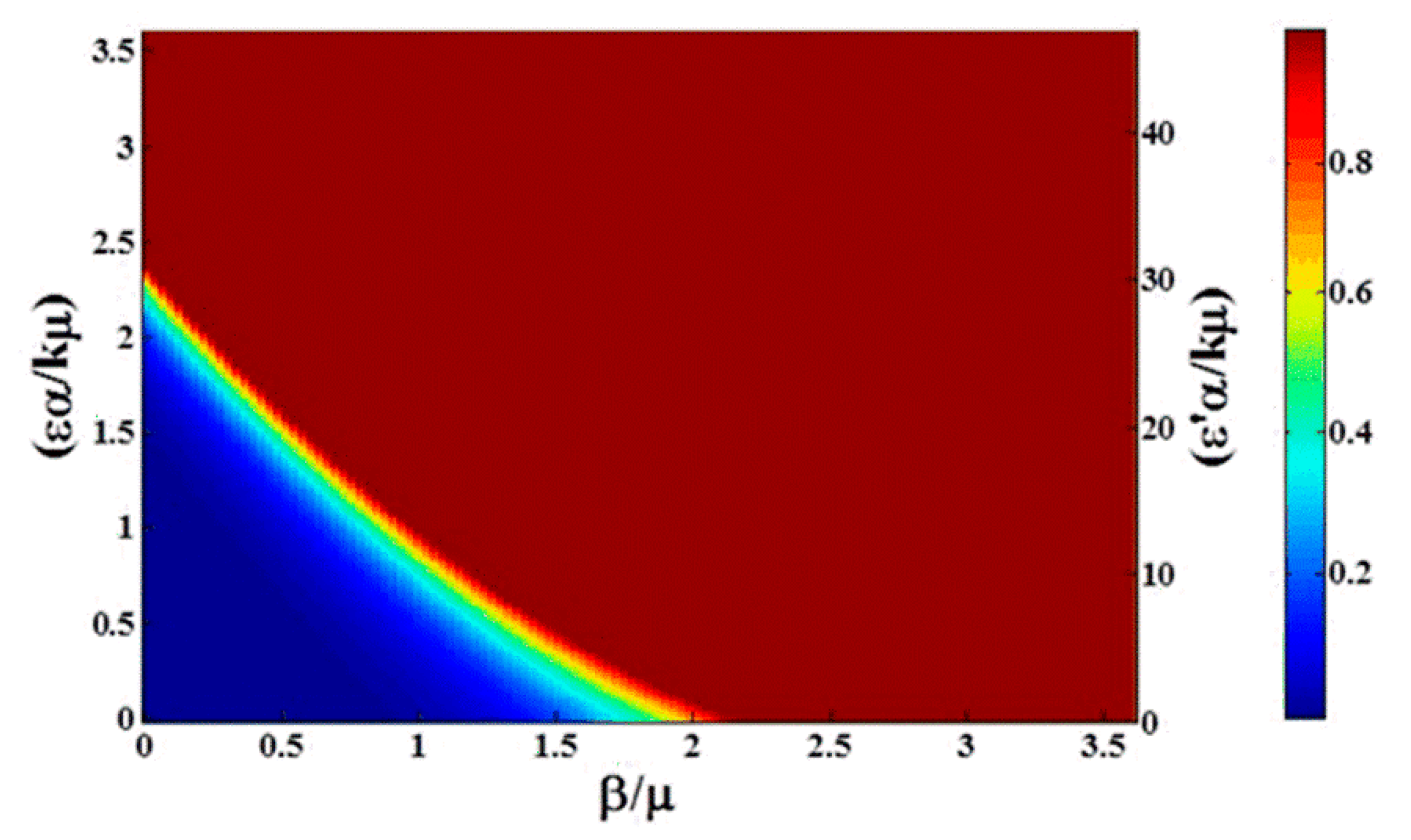
Effect of the dose response is demonstrated in Figure 6. Compared to Figure 3a, while there is still some asymmetry in the transition, the time to reach the steady state changes significantly. With low critical dose ($Q_0<1 )$ and high nonlinearity $(\nu >1)$, at t = 100 (days) the transition to a fully infectious population is both accelerated and sharpened. On the right-hand axis, we see the population becomes fully infectious for $\frac{ϵ\alpha }{\mu k}~2.0$, and the width of the transition in units of $\frac{ϵ\alpha }{\mu k}$ decreases from near 1 (Figure 2) to about 0.25 (Figure 6). Note the curvature of the contour lines in Figure 5. The right-hand axis in the figure is labeled with $\frac{{ϵ}^{\prime }\alpha }{\mu k}$, indicating explicitly the amplification in the rate of infection from environmental contamination due to the critical dose (Equation (11)). This can be helpful in predicting the impact of dose response for diseases where, once the bacterium is introduced to the environment, it spreads among the whole population very quickly, such as Campylobacter [13].

4. Discussions

A simple model is formulated to account for two different routes of veterinary infection: direct and indirect transmission. Mathematical analysis of the model in the steady state is accompanied by a numerical situation when the animal population has not reached steady state at the time of harvest. A dose-response version of the indirect transmission term is also included. The relative importance of the two routes to infection may depend strongly on farming practice in addition to the disease organism.

The general differential Equation (10) captures any combination of direct vs. indirect transmission, with and without dose response. It is certainly possible that some micro parasitic infections such as Campylobacter can transmit within a flock by more than one mechanism (i.e., the epidemiology may be driven by a combination of mechanisms). While it is ideal to have precise values for all the epidemiological parameters, experiments to determine the relative values of these parameters, and the relative contribution of each possible transmission pathway, can aid in planning the most effective interventions. For example, is the rapid spread of Campylobacter throughout an entire flock after thinning a result of stress weakening resistance and enhancing direct transmission, or is it a consequence of disturbed environmental contamination triggering a dose response in the remaining flock? Controlled production experiments that focus mainly on identifying the relative values of direct transmission rate $\left(\beta \right)$ and the rate at which new infections are produced via contaminated agents in the environment $\left(ϵ\right)$ would aid in learning the relative importance of transmission pathways and, therefore, the likely effect of proactive changes to farming practice. For example, controlled experiments could test the impact of cleaning flock containment areas before thinning, cleaning of containment areas with no thinning, sampling of individuals for testing throughout production, drinking water treatment and methodology, and ventilation rate throughout production, combined with monitoring of contaminated feces and water dispensers.

Together with data from controlled experiments, this simple yet flexible mode may aid in understanding the effectiveness of interventions for controlling the pathogens. For instance, the rate at which the environment is cleared of waste can parameterize the impact of cleaning strategies. As an open source model implemented in the Eclipse Framework, in the future the model can easily be extended to support the study of other interventions such as vaccination. Modeling the impact of vaccination would simply involve inclusion of a recovered or “removed” state, R, to the existing model. Another potential addition can be extending the current study to include the meta-population.