1. Introduction
In 1998, Shulgin et al. [
1], highlighted the potential of pulse vaccination strategy in eradicating some epidemics at relatively low values of vaccination compared to conventional strategies as theoretically proven also in [
2]. A theoretical examination of these results has been published after in [
3]. In the first mentioned reference and more recently in paper of Yang and Xiao in [
4], the authors discussed the effectiveness and importance of such vaccination regimes by referring to many theoretical and applicable results in the literature, namely the work of De Quadros et al. [
5] in case of poliomyelitis, and work of Albert Bruce Sabin in [
6] in cases of measles.
In 2001, Brauer et al. in [
7], referred to the pulse vaccination suggested in [
1,
2,
3] as a novel theoretical way to avoid recurring outbreaks of an epidemic. After the promising results presented in these references, many researchers showed more interest in the study of the complexity of epidemic models that involved this type of control measures, as in work of Alberto d’Onofrio in [
8] where it was numerically observed through the use of SEIR model that pulse vaccination program is slightly more efficient than the traditional continuous one, Zhou and Liu in [
9] with similar results in case of SIS model, Zeng and Chen in [
10] where it is understood that SIRS model becomes much more complex under such vaccination policies while these authors concluded the same with Sun in [
11] in case of SIR model. Extended studies with other different modeling frameworks have been published after, as in work of Gakkhar and Negi in [
12] where the authors studied the complexity of SIRS system with non-monotonic incidence rate, Zhang and Teng in [
13,
14] where the two references results both indicated that a large pulse vaccination rate will help to eradicate the disease using SEIRS and SIRVS systems respectively, Li and Cui in [
15] who compared between results of constant and pulse vaccination based on a comparison between pulse interval and a critical value of pulsing period, Zhao and Meng in [
16] that treated the application of pulse vaccination to vertically transmitted diseases as considered earlier in other references as in [
17,
18], Pei et al. in [
19] where it had been showed that the quarantine measure helps in eradicating the disease with similar conclusions as in [
13,
14] but through a delayed SEIQR model, Qiao et al. in [
20] exhibiting the potential of pulse vaccination strategy in eliminating viral infectious diseases, see also other interesting literature in [
21,
22,
23,
24].
There have been intensive research papers about optimal vaccination strategies obtained through optimal control methods for many diseases prevention, see ref. [
25] in case of dengue, ref. [
26] for Influenza, refs. [
27,
28] for malaria, ref. [
29] for Hepatitis B, ref. [
30] for Ebola, ref. [
31] for cholera. In these papers, the control is considered to be a continuous function in time, while the optimal control problem is resolved using classical theorems of sufficient and necessary conditions of optimality stated in [
32,
33] respectively. The optimization subject to such epidemic models, has mostly aimed to minimize the control policy cost associated with vaccination; however, as far as we know, there have been no studies that tried to resolve this problem in case of pulses with clearest and simplest methodology for better practicability. This means there is a need for a numerical method that applies exactly most findings of the theoretical calculus related to the necessary conditions of optimality with possibly clear analytical formulation of the sought optimal impulse control and without the help of any type of gradient methods. In 1978, Balquière provided in [
34], an impulsive version for these optimality conditions, but there is still a lack in research for larger interpretation of these results, especially in the numerical part. Here, we try to develop an algorithm that will simplify more the resolution of these problems, often referred to as optimal impulsive control problems [
35]. Further results about existence of solutions to these problems, have been discussed in [
36,
37].
We consider an optimal control problem subject to a state system that involves a finite number of impulse times in which an impulse control function is applied. More concretely, the control will represent the vaccination ratio as a variable in function of time and that is applied to a proportion susceptible to infection, while its optimal values will be sought at each time of vaccine application for better management of the pulse vaccination strategy.
To reach our purpose, we consider a susceptible-infected-removed (SIR) epidemic model with an additional compartment to represent the number of the vaccinated population. The proposed model is in the form of a differential system which contains a parameter that characterizes an impulse vaccination strategy followed for preventing the spread of an epidemic.
Since not every vaccine is necessarily
effective as explained in [
38], we choose to study dynamics of the considered population in this case. Then, an optimal impulse control strategy is suggested for this model using an impulse version of Pontryagin’s maximum principle. Finally, impulse progressive-regressive iterative schemes are used for finding the results.
2. Epidemic Control Model With Short-Term Immunity
2.1. Model Description in Continuous-Time Case and with Constant Control
In this part, we consider an epidemic control model where the vaccination strategy is described using a constant control parameter with the hypothesis that the used vaccines have a limited effect on people who receive it.
We need first to define the following four compartments
- :
the number of people susceptible to infection or who are not yet infected,
- :
the number of susceptible people who are temporary vaccinated so they cannot move to the removed class due to the limited effect of vaccine [
38,
39,
40],
- :
the number of infected people who are capable of spreading the epidemic to those in the susceptible and temporary controlled categories,
- :
the number of removed people from the epidemic.
For all
t belonging to an interval
and when the vaccination policy is only presented by a constant parameter of control
, the model takes the form of the following differential system
with initial conditions
,
,
and
and where
with
, giving the newborn people.
is the fraction of controlled people with “a” modeling the reduced chances of a susceptible individual to be controlled.
Also, with the infection transmission rate, is the natural death rate, is the infection transmission rate even in the presence of with “b” modeling the reduced chances of a temporary controlled individual to be infected, and is the recovery rate.
The population size N is constant because , hence, knowing that .
We note that will denote no vaccination and will denote the use of vaccination with an initial number of susceptible people .
In [
38], the authors devised a discrete-time version of (1) under the reason that in epidemics, data are collected at discrete times, while in [
39,
40], the model has been limited to its following continuous-time version
However, since vaccinations are often neither given continuously, nor at daily or very close discrete times, an impulse version of such models, seems more realistic. This leads us to think about devising an epidemic model that takes into account such considerations while providing theoretical and numerical steps for the resolution of an impulse optimal control problem.
Let first present the model (1) when there is use of pulse vaccinations.
2.2. Model Formulation in Impulsive Case with Control Function
Let , , …, be the times the vaccinations are applied. n is their total number.
Since our goal in this paper is to find the optimal values of pulse vaccination rate
at
, then, we start with converting the continuous-time control
into the discrete summation
. The continuous-time model in (
2) becomes defined by the following system with impulse vaccinations
where
is a type of Dirac-delta function and each term of the summation above realizes the following property
In fact, the summation
in (
3) can be considered to be a sum of weighted Kronecker-delta functions as the term (
4) is a shifted delta function with a specified weight. More generally, the summation as defined here, refers to a bounded discrete signal and the delta function is defined in this case by
while an integral form refers to real continuous-time case and the delta function is defined as
with the famous properties
,
and
, but this is not the case here.
Finally, and contrary to the form of control in (
2),
will be defined as the whole sequence in one single function
and when seeking its optimal values, we will need the values of
.
Thus, we understand the following conditions.
If
, then the system (3) is changed to
and if
, then we can obtain the following equations
where
representing the vaccination time and
the impulse control at this time, while
,
,
and
are defined as the old numbers of susceptible, vaccinated, infected, and removed people respectively, while
,
,
and
defining these same numbers just after
. Thus, (
8) means we have abandoned the old vaccination and used a new vaccination for the number of susceptible people
.
Before the presentation of our optimal control approach, let provide first a result about the stability of these systems when the control parameter is still defined as a constant rate.
3. Basic Reproduction Number
In system (
7) and (
8), since the three first equations are independent of the last equation, the study of stability can be reduced and done for the following system
which has a unique and piecewise continuous solution in
[
41,
42].
If there is no infection, i.e.,
then
, and system (
9) becomes
whose solution on
with
h, the time between two consecutive impulse vaccinations, is
with
and
.
In fact, the first equation in (
10) implies that
as noted earlier in the definition of
in
Section 2. By passage to the integral with letting just
in the right-hand side, we obtain,
, then,
, which gives
. At
, we have
, then,
and by replacing it in
, we obtain the result. As for the second equation, this is simpler after integration and we can find that constant
c is equal to
.
Let
and
, we can solve
,
and find a unique positive periodic solution
of system (
10).
where
Then, we find the basic reproduction number associated with system (
9) as
Based on similar results in [
43,
44,
45,
46,
47], we announce the following theorem
Theorem 1. The disease free periodic solution is globally asymptotically stable if and the disease is permanent if meaning the existence of a positive constant such that any solution of system (9) with initial values satisfies . This theorem shows that system (
9) exhibits similar threshold dynamics to the continuous-time case treated in [
39].
4. Optimal Impulse Control Approach
4.1. Theoretical Framework
In this part of paper, we define our objective by determining the optimal values of the impulse control that minimizes a given criterion, but before this, we present hereafter the theoretical steps for reaching this goal.
With a combination of results in [
48,
49], we try here to derive an analogous necessary conditions of optimality that will be associated with our particular form of the impulsive system (
3) which does not contain any continuous-time control as usually taken into consideration in general theoretical formulation in the literature, but only an impulse control here.
We start then first by presenting a general formulation of our optimal control problem that can be adapted to the form (
7) and (
8) as follows
subject to
where
x is the state variable, a piecewise continuous function of time, and
is the impulse control variable.
n is the number of pulses,
is the instant of the ith pulse and
,
are the instants just before and after the impulse, (i.e.,
,
represent the first and second limit sides of
x respectively). The final time is noted
while
is the instant that comes just after
T.
The system gain is given by , is the gain function associated with the ith pulse, and is the final cost function associated with the system just after T.
Finally, is the continuous change of the state variable through time between pulses points and is the function that represents the instantaneous or finite change of the state variable when there is a pulse.
We admit that is a bounded convex control set, and we impose that and G are continuously differentiable functions in x on and in on , is continuously differentiable in on ,and that g and G are continuous on t. Finally, when there is no pulse, i.e., , we assume that for all x and t.
As we have defined the general formulation of our objective that can be associated with the form of impulsive system (
3), we follow similar steps as in [
50,
51,
52] to obtain the following theorem which states the necessary conditions of optimality associated with our special case of optimal impulse control problem (
15).
Theorem 2. Let be optimal solutions of the maximization problem (15), then there exists an adjoint variable such that the following conditions are satisfied In the points of pulses, we have Proof. In [
34], the author developed a maximum principle theorem for necessary conditions of optimality to resolve the problem (
15) but with a continuous-time control function in the state equation when
. Here, since we have no continuous-time control in system (
7), we proceed in our generalized form as follows.
First, we consider the Hamiltonian function defined by
and the impulse Hamiltonian function defined by
where
represents the adjoint state variable.
Please note that (
16) is equivalent to the existence of the adjoint system in the classical continuous-time version of maximum principle [
33]. As for (
17) and (
18), it is directly obtained from results in [
34] and the only difference here in (
17) is that the sign ≤ is replaced by ≥ because (
15) is presented as a maximization problem. An analogous condition for the Hamiltonian
H is necessary if the state equation also includes a continuous-time control, otherwise, the only sought optimal control here is the impulse one that intervenes when
. In this remark, a function
still has a meaning because instead of defining an optimal trajectory
for both continuous and impulse controls,
will be just associated now to
only. This also implies that another condition may involve both classical and impulse Hamiltonian functions
H and
and which can be defined by
Since we will deal with an autonomous system, the condition (
19) is reduced to
and it means that
H is continuous at all times where
is applied [
49]. □
4.2. Optimal Impulse Control Problem
The most evident objective in epidemic control as defined for models in [
38,
39], concerns the minimization of the number of infected people while minimizing the cost of vaccination. Thus, for our case, we choose to define our objective function to be minimized as
In other words, we are seeking an optimal control
such that
subject to
Or, our optimal pulse control problem can be stated as follows
To resolve problem (
22), we follow these steps.
First, we construct the Hamiltonian
H without control as the function defined as
and second, we construct the impulse Hamiltonian function
defined as
We prefer the notation to just to avoid any ambiguity especially when we will need the derivative of this function with respect to function of infection I.
We can announce the impulse maximum principle as follows.
Theorem 3. Given an impulse optimal control where and which minimizes (20) along with the optimal trajectories , , and associated with the differential system in (22), then there exist adjoint variables , as notations of and which satisfy for the following adjoint differential systemwith the transversality conditions , and we have, Proof. We have the Hamiltonian function
H is defined in (
23) as
Then, using the impulse version of Pontryagin’s maximum principle in [
48], then we have, for
while the transversality conditions defined as minus the derivative of the final gain function with respect to the state variables S,
, I, and R. Since the final gain function in (
20) does not contain any term of these variables, then
,
.
Since the impulse Hamiltonian function
is defined in (
24) as
Then, we have also at
The optimality condition at implies that .
Then, after setting
, we have
By using the bounds of control defined in (
22) and similar detailed calculus as in [
38,
39], we obtain the following characterization
□
5. Numerical Results
As mentioned in introduction, we aim in this numerical part, to propose a numerical method that applies exactly the findings of the last theorem. Since all necessary conditions of optimality along with the characterization of the optimal control, are all found explicitly in this theorem, we do not need any type of gradient method.
In fact, the four steps of numerical calculus associated with the resolution of our impulse optimal control problem (
22)–(
25), are described in Algorithm 1.
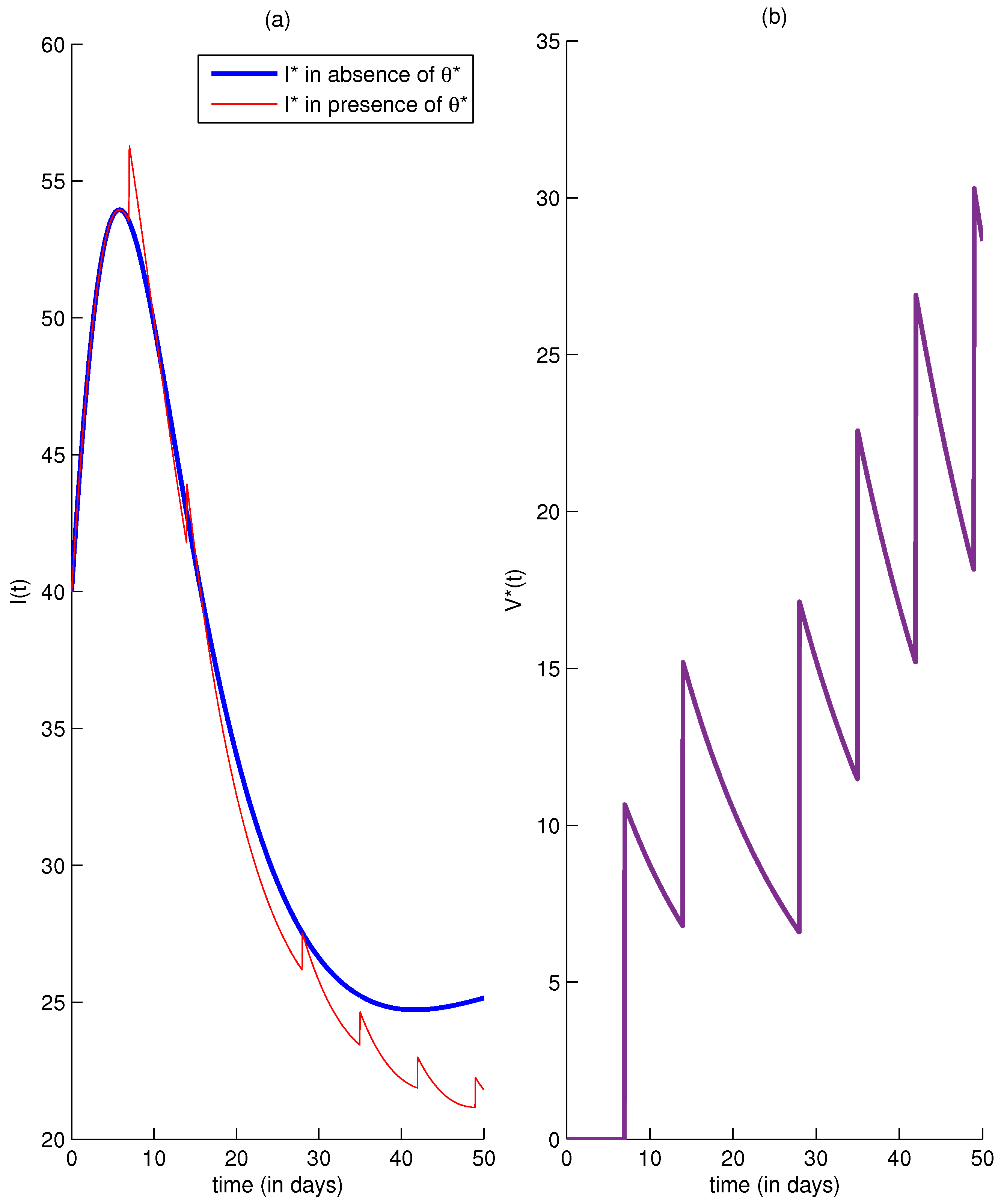
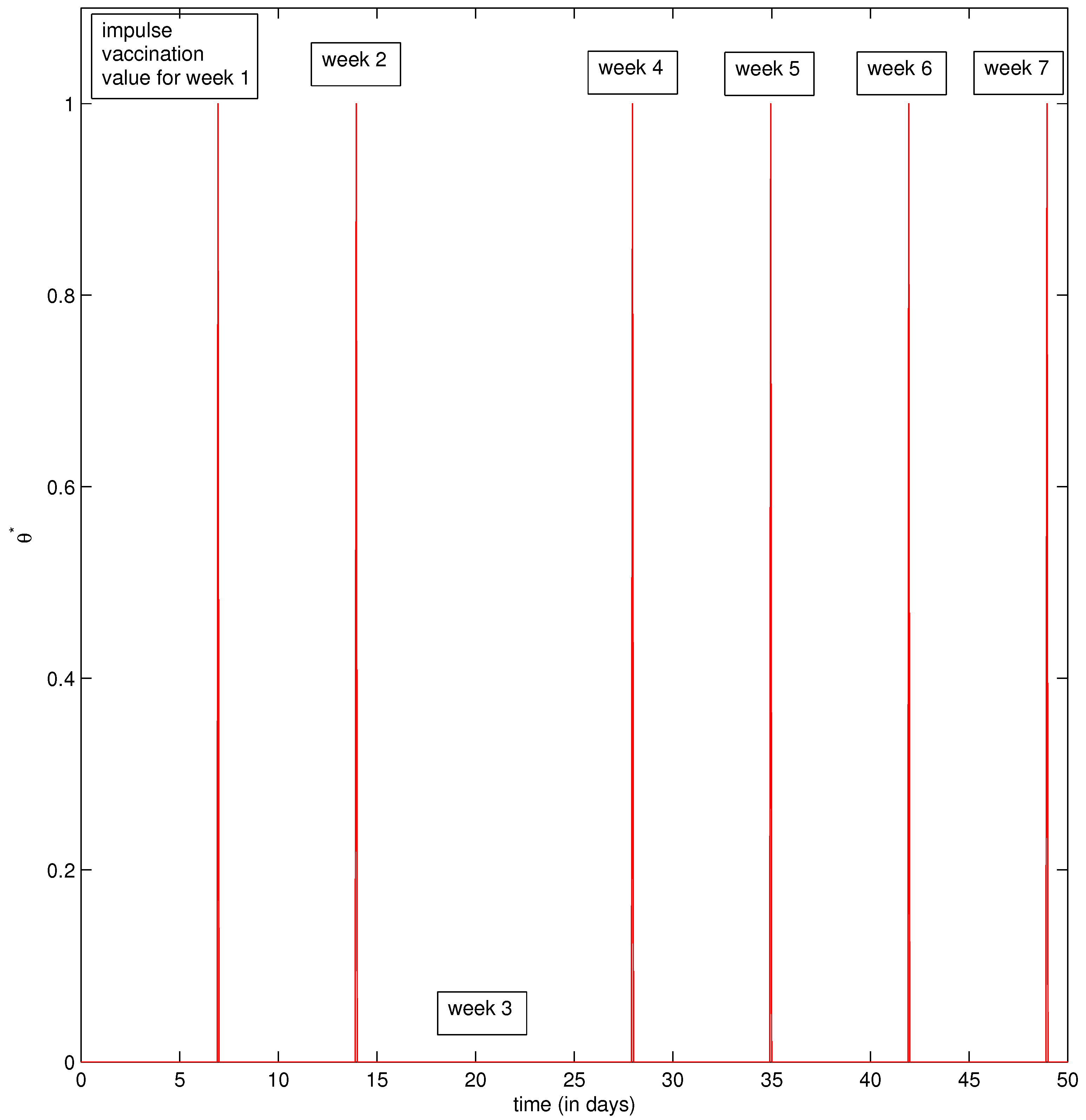
Figure 1 and
Figure 2 depict
dynamics in the absence and presence of control. As for
Figure 3, we exhibit the recommended pulses.
When we talk about the case when there is no vaccination strategy, we mean that we deal with the following continuous-time SIR differential equation
for all time
, and this system clearly describes the continuous spread of the epidemic in a population without any control intervention. The behaviors of
and
for all time
in this case, are presented with the blue curves in the three figures below. As for the case when we follow an impulse vaccination strategy subject to (
22), the behaviors of
and
for all time
, are presented with the red curves.
| Algorithm 1: Resolution steps of the two-point boundary value optimal control problem (22)–(25) |
Step 0: Guess an initial estimation to . Step 1: Use the initial condition , , and and the stocked values by . Find the optimal states , , and which iterate forward in (23) in the two cases when and when . A progressive fourth order Runge-Kutta scheme is incorporated for finding the state solutions from 0 to a fixed number of iterations m. Step 2: Use the stocked values by and the transversality conditions (26). Find the adjoint variables for which iterate backward in (25) when and in (26) when . A regressive fourth order Runge-Kutta scheme is incorporated for finding the costate solutions from m to 0. Step 3: Update the control using new S, V, I, R and for in the characterization of as presented in(27) Step 4: Test the convergence based on the forward-backward sweep method criterion. If the values of the sought variables in this iteration and the final iteration are sufficiently small, check out the recent values as solutions. If the values are not small, go back to Step 1.
|
From most epidemiological data we have revised until now, especially in the case of controllable epidemics that appeared at specific seasons, we concluded that it is preferable to avoid parameters values that can lead to claiming the occurrence of an exponential increase of infection and deny the exponential decrease that just comes after the infection reaches its maximal peak, we also prefer to not analyze the advantage of our approach on fractions, but instead on numbers of individuals. The parameters values that will be considered here, may certainly help to understand this phenomenon. In fact, there was always an urgent control measure which aimed to prevent the spread of epidemics with the best available resources. The problem as mentioned in [
7], is that we cannot be sure that the infection will not appear again since in practice, it is nearly impossible to vaccinate most susceptible individuals of a population because not all people would come to be vaccinated and not all vaccinations are successful [
7,
38,
39,
40]. In the same context, El Kihal et al. discussed other possible reasons such as the constraint of limited resources as in [
38] or infodemics as in [
53]. Thus, a better way to avoid the recurrence of a disease outbreaks, is to follow a control strategy based on pulsed vaccinations.
From
Figure 1a, we can observe that the susceptible number S decreases exponentially towards 37 individuals and this is mostly due to infection plus natural death as it can be understood from the first equation in (
29). In fact, the number of infectives I in
Figure 2a increases exponentially towards an important number of more than 54 individuals in during the first week and decreases thereafter to just 25 individuals in the sixth week because of the natural death and natural recovery as it can also be deduced from second equation of (
29), but this also may be due to another type of control intervention missed here but not sufficient as infection remains important and needs to be controlled.
In
Figure 1a, the optimal state
decreases rapidly towards 38 individuals in the first week and this value is smaller than the one taken by S because of the optimal impulse control intervention. However, once we go more forward in time, the effect of control becomes negligible and this causes a slight increase of
between 10 and 12 days, and then an simultaneous increase of the function
in
Figure 2a in the same period to 57 individuals in the first week but decreases again to 27 people and this implies to some small increases of
compared to S, and we remark once there is a vaccination interruption just after the time of impulse,
does a slight jump again and again causing repeated small decreases of
. Simultaneously, the number of removed people R in
Figure 1b increases to 57 people before the third week because of the natural recovery or any effect of other missed control policy in removing the infectives, while
reaches a value that is higher than this number with a maximal peak equaling to 62 in the third week.
From
Figure 3, we can show that vaccination is recommended in all weeks except on the third time of impulsion. The optimal values of controls take the value 1 as maximal peak in these weeks while it is zero in week 3. In fact, as we can observe from
Figure 1b and
Figure 2a, since R and I functions do not oscillate during days that are
and
but they increase and decrease in this period respectively, then, there is no need to introduce any control in the third week.
The main result we can recapitulate from these first three figures is that all
and
oscillated in all times of pulsed vaccinations, and once a vaccination is stopped, the infection goes up again in repeatedly increases with differentiated peaks, and respectively, the level of recovery goes down many times. As for
in
Figure 2b, it is very small because of the small values
has taken in most times of vaccination.
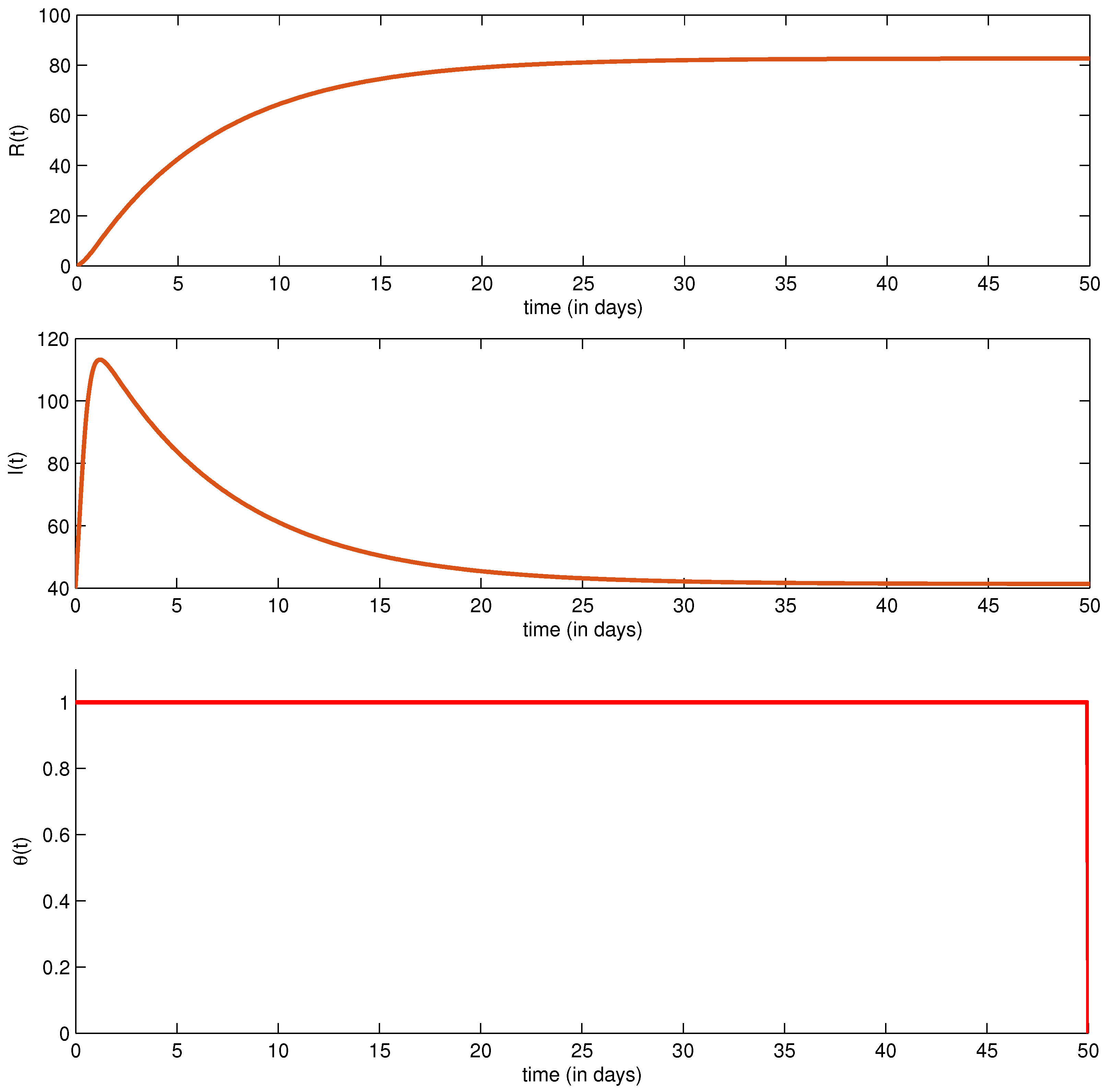
6. Discussion and Conclusions
The introduction of a continuous-time control in system (
29) as done in [
39], would seem less important than the use of an impulse control when it comes to subject of vaccination since we know that vaccines are injected on a discrete basis. In fact, with an optimal impulse control strategy, we may succeed to obtain a reduction in the number of infected people (resp. an augmentation in the number of removed people) without following a control policy at all continuous-time t. From
Figure 4, we remark there are no oscillations in the curves of I and R functions since there is no interruption in the control along
. Although less realistic, the continuous-time control also shows a positive effect on shape of R (resp. on shape of I) as the recovery has stabilized (resp. the infection has decreased) to small values a little before than the cases in
Figure 1b and
Figure 2a. However, vaccination managers would surely choose recommendations of
Figure 4 since the main goal of the minimization problem (
21) with respect to the definition in (
20) has been reached in similar way with even many vaccination rest periods, and this also meets the conclusions of [
8,
9] that impulses are slightly better than administrating vaccines continuously. This is to say there is no need to have an optimal control in its maximal bound suggested overall t as observed in
Figure 4. Talking about the bound 1 as maximal suggested value for the control either in
Figure 4 or
Figure 3, we mention this is due to the number of infected people that despite the decrease, its minimal value is still around 40. Thus, we try to resolve and discuss this problem in the two following figures.
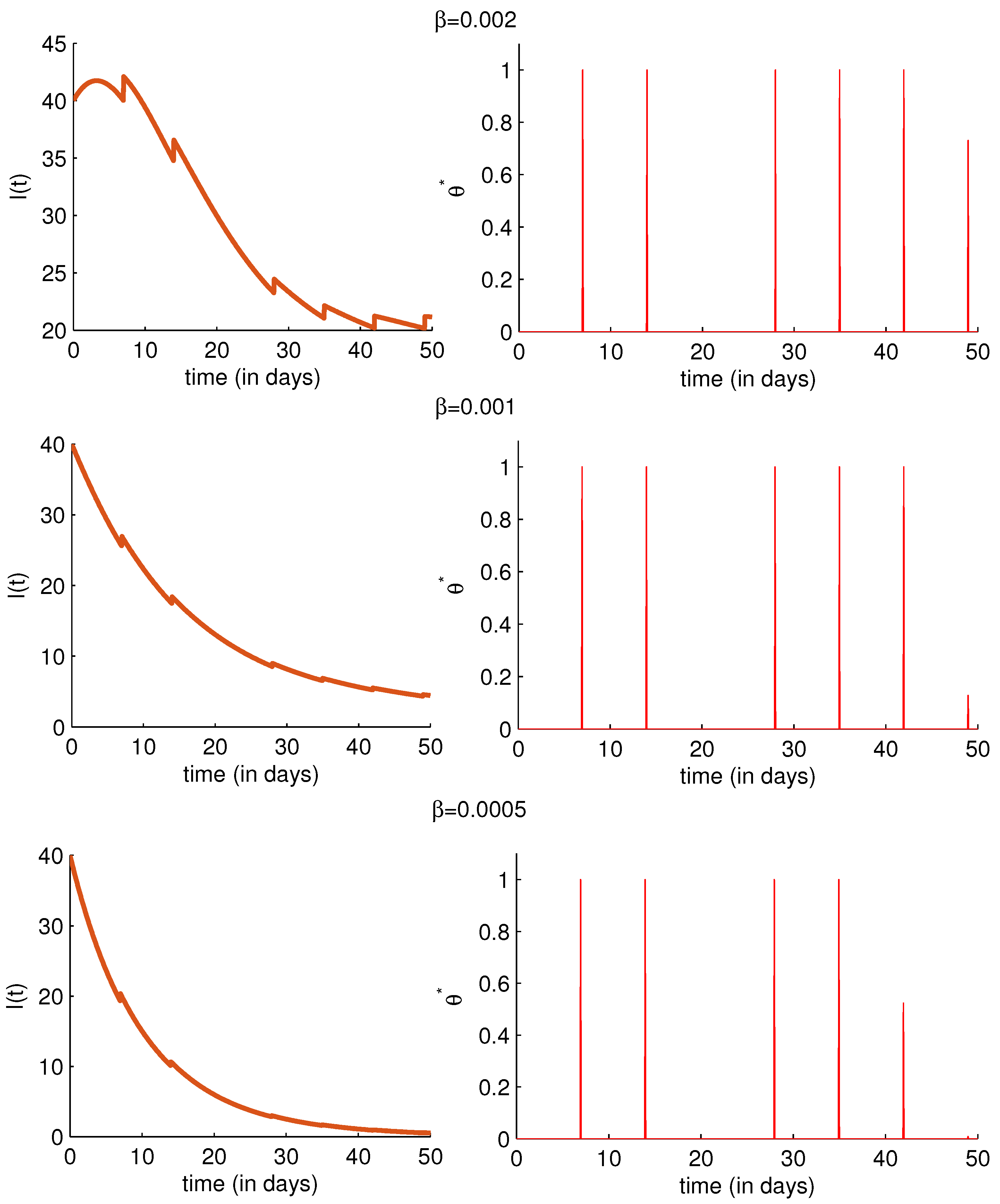
In
Figure 5 and
Figure 6, we discuss the behaviors of
function and the recommended impulse controls when the infection transmission rate
β varies. In
Figure 5, when
, we can observe that the number of infected people decreases now to 20 individuals as minimal value, and simultaneously, the value of the optimal impulse control in the last week is reduced to 0.75. As for the case when
,
decreases to only 5 individuals while the value of the optimal control takes only 0.14 in the last week. In the last case of the same figure, we could now say that infection could be eradicated as long as we move forward in time since
is equal to approximately zero in the 49th day even no impulse control is suggested in this time but only a value of 0.55 in the previous week is sufficient, without forgetting the ones values of other controls in the first weeks.
As we wonder whether there is a possibility to avoid more impulses for lesser costs, we found in
Figure 6 that by affecting smaller values to
β than in the previous figure, this may be achieved. In fact, when
, the infection reaches the zero value in the 35th day while there is no suggested control in the last and sixth weeks with negligible value of the control in week 5 and very small value in week 4, and with the value 1 as maximal peak in the first week only and the value 0.64 in the second one. Similar results are obtained when
with some reduction of 0.1 and 0.2 in the two first weeks, respectively. As for the last case, when
, the two first impulse optimal controls take only 0.22 and 0.08 with no recommendations for other weeks. Thus, we deduce that the more the infection transmission rate is important, the fewer impulse controls are required to introduce and the infection reaches the zero value in minimal time.
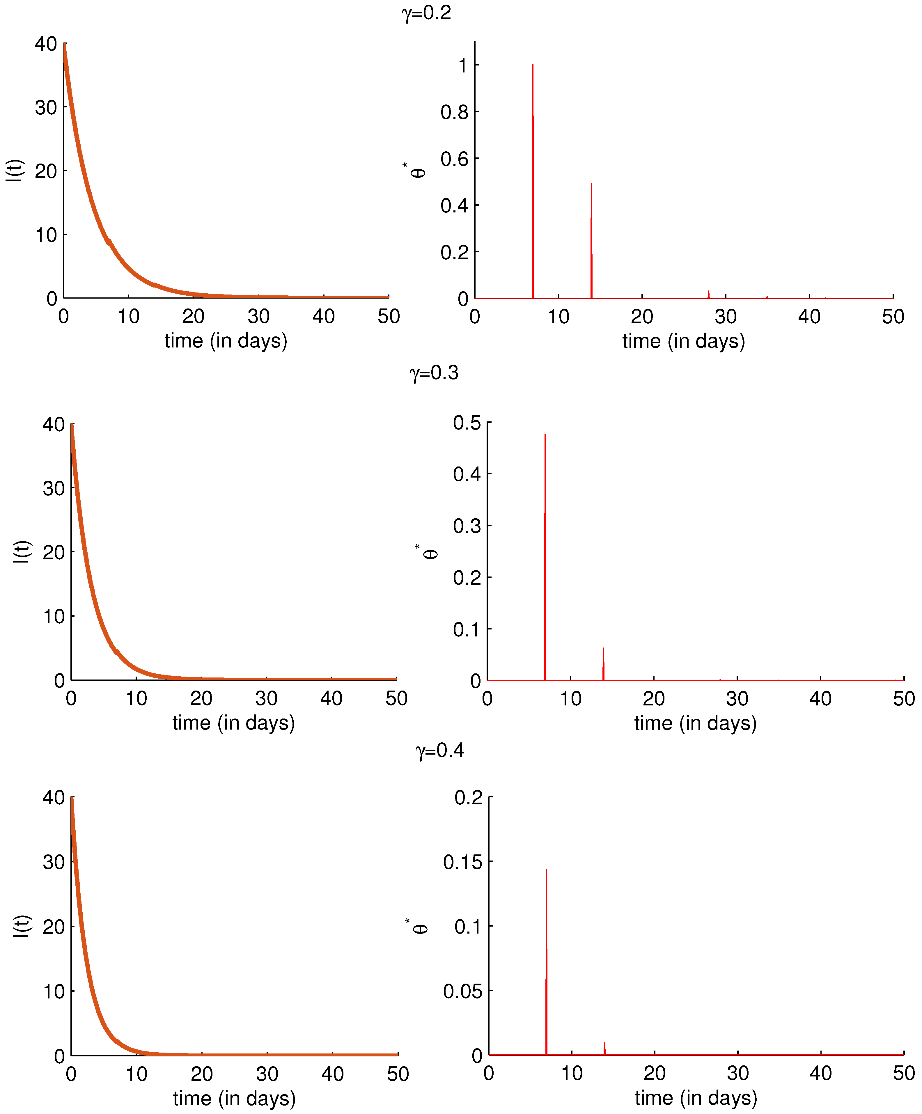
In
Figure 7, we discuss the behaviors of
function and the suggested impulse controls when the recovery rate
γ varies. When
, the infection decreases towards the zero value after only 20 days with the requirement of only two impulse controls taking the values 1 and 0.5 as maximal peaks in the two first weeks, respectively. Now, when
, the infection lasts only 14 days and disappears with the introduction of only two impulse controls taking the values 0.48 and 0.07 in weeks 1 and 2, respectively. In the last case, when
, the infection is eradicated after only 11 days with the effect of only one control in the first week and that takes a very small rate of 0.15 while a second control appears negligible in week 2. Thus, we deduce that the more the recovery rate is important, the fewer impulse controls are recommended while
function may reach 0 even before the second week of intervention.
From all the results exhibited in the last three figures with different values of
γ and
β, we can now agree with the conclusions of [
13,
14,
19] that large pulse vaccination rate will help to eradicate the disease, but this remains correct only if the transmission rate is not very important since in the example of
Figure 1, despite the distinguishable decrease of infection with respect to the case without control, the number of infection remains important even if the optimal control in
Figure 4 takes its maximal bound.
Finally, the optimal control strategy subject to our SVIR hybrid epidemic model, showed promising results when applied for first time in this form to the problem of pulsed vaccinations. Such optimization approaches can be extended to other applications with better description of policies that are not followed on continuous basis but rather introduced just between fixed time intervals. In future work, the potential of this impulse control strategy may also be discussed in case we focus more on most promiscuous individuals only, as deduced through targeted immunization approach suggested in [
54]. Another interesting work that can meet the idea of impulse vaccination, is in [
55] where the authors found that the influential nodes are not vaccinated on continuous basis but just repeatedly.

