Backward Bifurcation and Optimal Control Analysis of a Trypanosoma brucei rhodesiense Model

Abstract

In this paper, a mathematical model for the transmission dynamics of Trypanosoma brucei rhodesiense that incorporates three species—namely, human, animal and vector—is formulated and analyzed. Two controls representing awareness campaigns and insecticide use are investigated in order to minimize the number of infected hosts in the population and the cost of implementation. Qualitative analysis of the model showed that it exhibited backward bifurcation generated by awareness campaigns. From the optimal control analysis we observed that optimal awareness and insecticide use could lead to effective control of the disease even when they were implemented at low intensities. In addition, it was noted that insecticide control had a greater impact on minimizing the spread of the disease compared to awareness campaigns.

1. Introduction

Human African trypanosomiasis (HAT) is one of the neglected tropical diseases (NTDs) that affect humans and animals in sub-Saharan Africa [1]. More than 20 species of Glossina tsetse flies are responsible for the transmission of the two parasites associated with the disease: Trypanosoma brucei rhodesiense and Trypanosoma brucei gambiense [1]. Although these two parasites represent different pathological entities, they are both classified under the term HAT [2]. T.b. gambiense is found in West and Central Africa, while T.b. rhodesiense occurs only in the East and South of the African continent [1]. Global estimates report 70,000 HAT cases (range: 50,000–70,000) based on a total number of 17,500 new cases reported per year worldwide [3]. With more than 60 million in sub-Saharan Africa considered to be at risk of infection, how to prevent, control and possibly eradicate this disease remains one of the important topics from many points of view, including medical science and mathematics.

Since the pioneering work of Kermack and McKendrick [4] on compartment modeling, numerous mathematical models have been proposed to investigate the transmission dynamics of several infectious diseases (e.g., [5,6,7,8,9,10,11] and references therein). These studies and several other models have certainly produced many useful results and improved the existing knowledge on several infectious diseases, such that mathematical modeling has become an important tool in analyzing the spread and control of infectious diseases. In particular, several mathematical models have already been proposed to investigate the complex epidemic and endemic behavior of human African trypanosomiasis [12,13,14,15,16,17,18,19,20,21,22,23,24,25,26,27]. For example, Hargrove et al. [12] modeled the control of trypanosomiasis caused by Trypanosoma brucei rhodesiense in multiple hosts. Their model predicted that treating cattle with insecticide would be generally more effective than treating cattle with drugs. In addition, Moore et al. [14] utilized a system of ordinary differential equations to explore the impact of climate change on Trypanosoma brucei rhodesiense dynamics. Results from their framework suggested that climate change could lead to 46–77 million additional people being at risk of exposure to HAT infection by 2090. These studies and those cited therein have undeniably produced many useful results and improved the existing knowledge on HAT dynamics.

Despite these efforts in the modeling and analysis of Trypanosoma brucei rhodesiense dynamics, several important questions regarding the transmission and control of the disease remain to be answered. For example, to what extent will awareness and insecticide use combined alter short- and long-term transmission and control of HAT? Thanks to Hargrove and co-workers [12], we are now aware that insecticide use has a greater impact on controlling the disease compared with the treatment of cattle with drugs. The key question is, if this intervention were to be combined with awareness campaigns, would this approach yield a significant change in Trypanosoma brucei rhodesiense? This is the key question that this study aimed to explore. There is no doubt that continuous advancement in information and communication technology (ICT) in recent years has greatly improved the level of information dissemination. In addition, media campaigns are known to be useful public health tools globally [28,29]. In particular, mass media campaigns have the potential to alter people’s health behavior in the absence of multiple channels of communication [29,30]. Therefore, as suggested by Leak [31], understanding the impact of these intervention strategies on disease and vector population dynamics is a potential area for modeling and further development of existing models. Motivated by the discussion above, in this paper we seek to use optimal control theory to investigate the effects of awareness campaigns and insecticide use on the spread and control of Trypanosoma brucei rhodesiense. Stone and Chitnis’ [16] model of HAT transmission, which does not incorporate an animal reservoir, does not effectively capture the dynamics of the disease. Hence, we propose a framework that demonstrates interplay between the vectors and multiple host species (human and animals). By incorporating the vectors and multiple hosts, our framework will be isomorphic to some of the earlier studies [12,14,16,23,27].

This paper is organized as follows. In Section 2, the methods and results of the study are presented. in particular, the Trypanosoma brucei rhodesiense model is formulated and analyzed. The analysis included the computation of the basic reproduction number and the existence of model steady states. The impact of two controls—awareness campaigns and insecticide use—as disease control measures against Trypanosoma brucei rhodesiense infection was also investigated. In addition, numerical simulations were conducted to support analytical findings. Finally, discussion and conclusions round up the paper.

2. Methods and Results

2.1. Model Formulation

The proposed model considers two hosts (i.e., animals and humans), subdivided into: susceptible $S_i\left(t\right)$, clinically infected $I_i\left(t\right)$ and removed $R_i\left(t\right)$, for $i=a$ and h-representing the animal and human, respectively. Thus the host population at time t is given by $N_i=S_i\left(t\right)+I_i\left(t\right)+R_i\left(t\right).$ Furthermore, the total tsetse vector population at time, denoted by $N_v\left(t\right)$, constitutes the susceptible $S_v\left(t\right)$ and infectious $I_v\left(t\right)$ populations. Once infected, vectors are assumed to remain infectious for their entire lifetime. Through mass media campaigns humans are assumed to become aware of the disease and those who become aware are assumed to have negligible chances of being infected. Hence, in our framework we introduced a constant rate ${\theta }_h$ to account for the transition of individuals from the susceptible compartment to the removed class. Thus, the removed compartment for humans comprises individuals who were successfully treated and those who have become aware of the disease. With the passage of time these individuals may lose their awareness and become susceptible to infection again. In order to model disease transmission from the host to the vector and vice versa, we propose the following forces of infection:

$$\begin{array}{c}{\displaystyle {\lambda }_h\left(t\right)=\frac{{\beta }_{vh}{I}_v\left(t\right)}{N_v\left(t\right)},{\lambda }_a\left(t\right)=\frac{{\beta }_{va}{I}_v\left(t\right)}{N_v\left(t\right)},{\lambda }_v\left(t\right)=\frac{{\beta }_{hv}{I}_h\left(t\right)}{N_h\left(t\right)}+\frac{{\beta }_{av}{I}_a\left(t\right)}{N_a\left(t\right)},}\hfill \end{array}$$

where parameter ${\beta }_{vi}$ ($i=a,h$) denotes the transmission rate of HAT disease from an infected tsetse vector to a susceptible host i given that effective contact between the two occurs; ${\beta }_{iv}$ represents disease transmission from infected host i to a susceptible vector given that effective contact between the two occurs. In addition, parameters ${\mu }_a$, ${\mu }_h$ and ${\mu }_v$ represent the inflow of new individuals into the susceptible animal, human and vector populations, respectively, through birth, and are assumed to be equal to the natural mortality rates for each population. There is no vertical transmission of the disease in either the host or vector. Infected animals and humans recover at rates ${\alpha }_a$ and ${\alpha }_h$, respectively, and they become susceptible to infection at rates ${\gamma }_a$ and ${\gamma }_h$, respectively.

The proposed model is summarized by the following equations, where the prime ${(}^{\prime })$ denotes the derivative of the component with respect to time:

$$\left\{\begin{array}{ccc}{\displaystyle S_h^{\prime }\left(t\right)}\hfill & =\hfill & {\mu }_h{N}_h\left(t\right)-{\lambda }_h\left(t\right)S_h\left(t\right)-({\mu }_h+{\theta }_h)S_h\left(t\right)+{\gamma }_h{R}_h\left(t\right),\hfill \\ {\displaystyle I_h^{\prime }\left(t\right)}\hfill & =\hfill & {\lambda }_h\left(t\right)S_h\left(t\right)-({\mu }_h+{\alpha }_h)I_h\left(t\right),\hfill \\ {\displaystyle R_h^{\prime }\left(t\right)}\hfill & =\hfill & {\theta }_h{S}_h\left(t\right)+{\alpha }_h{I}_h\left(t\right)-({\mu }_h+{\gamma }_h)R_h\left(t\right),\hfill \\ {\displaystyle S_a^{\prime }\left(t\right)}\hfill & =\hfill & {\mu }_a{N}_a\left(t\right)-{\lambda }_a\left(t\right)S_a\left(t\right)-{\mu }_a{S}_a\left(t\right)+{\gamma }_a{R}_a\left(t\right),\hfill \\ {\displaystyle I_a^{\prime }\left(t\right)}\hfill & =\hfill & {\lambda }_a\left(t\right)S_a\left(t\right)-({\mu }_a+{\alpha }_a)I_a\left(t\right),\hfill \\ {\displaystyle R_a^{\prime }\left(t\right)}\hfill & =\hfill & {\alpha }_a{I}_a\left(t\right)-({\mu }_a+{\gamma }_a)R_a\left(t\right),\hfill \\ {\displaystyle S_v^{\prime }\left(t\right)}\hfill & =\hfill & {\mu }_v{N}_v\left(t\right)-{\lambda }_v\left(t\right)S_v\left(t\right)-{\mu }_v{S}_v\left(t\right),\hfill \\ {\displaystyle I_v^{\prime }\left(t\right)}\hfill & =\hfill & {\lambda }_v\left(t\right)S_v\left(t\right)-{\mu }_v{I}_v\left(t\right).\hfill \end{array}\right.$$

(1)

Table 1. Description of parameters used in system (1). HAT: human African trypanosomiasis.

Symbol	Description	Value	Units
${\beta }_{hv}$	Transmission rate of HAT disease from infected human to susceptible vector	$0.011715$	day${}^{-1}$	[14]
${\beta }_{av}$	Transmission rate of HAT disease from infected animal to susceptible vector	$0.011715$	day${}^{-1}$	[14]
${\beta }_{vh}$	Transmission rate of HAT disease from infected vector to susceptible human	$0.002739$	day${}^{-1}$	[14]
${\beta }_{va}$	Transmission rate of HAT disease from infected vector to susceptible animal	$0.002739$	day${}^{-1}$	[14]
${\gamma }_h$	Progression rate of human population from recovered to susceptible class	${\displaystyle \frac{1}{90}}$	day${}^{-1}$	[23]
${\gamma }_a$	Progression rate of animal population from recovered to susceptible class	${\displaystyle \frac{1}{75}}$	day${}^{-1}$	[23]
${\theta }_h$	Rate at which humans become aware of the disease	0.2	day${}^{-1}$
${\mu }_h$	Natural mortality rate of human population	${\displaystyle \frac{1}{365\times 50}}$	day${}^{-1}$	[23]
${\mu }_a$	Natural mortality rate of animal population	${\displaystyle \frac{1}{365\times 15}}$	day${}^{-1}$	[23]
${\mu }_v$	Natural mortality rate of vector population	${\displaystyle \frac{1}{33}}$	day${}^{-1}$	[23]
${\alpha }_h$	Recovery rate of infected human	${\displaystyle \frac{1}{30}}$	day${}^{-1}$	[23]
${\alpha }_a$	Recovery rate of infected animal	${\displaystyle \frac{1}{25}}$	day${}^{-1}$	[23]

presents the model parameters and their baseline values. The baseline values for these parameters were adopted from the work of Moore et al. [14] and Ndondo et al. [23]. In their studies, Moore et al. [14] and Ndondo et al. [23] proposed mathematical models with interplay between the vectors and multiple host species. In particular, the host species considered were humans and animals (cattle), hence the parameter values from these studies can also be used in this study.

From (1) we have $N_i^{\prime }\left(t\right)=0$ for $i=a,h,v$, hence without loss of generality we can use a dimensionless system to explore the dynamics of the disease. Now, to normalize the populations, let

$$\begin{array}{ccc}{s}_h\left(t\right)\hfill & =& \frac{S_h\left(t\right)}{N_h},i_h\left(t\right)=\frac{I_h\left(t\right)}{N_h},r_h\left(t\right)=\frac{R_h\left(t\right)}{N_h},s_a\left(t\right)=\frac{S_a\left(t\right)}{N_a},\hfill \\ i_a\left(t\right)\hfill & =& \frac{I_a\left(t\right)}{N_a},r_a\left(t\right)=\frac{R_a\left(t\right)}{N_a},s_v\left(t\right)=\frac{S_v\left(t\right)}{N_v},i_v\left(t\right)=\frac{I_v\left(t\right)}{N_v}.\hfill \end{array}$$

Therefore, the dimensionless system has the form:

$$\left\{\begin{array}{ccc}{s}_h^{\prime }\left(t\right)\hfill & =\hfill & {\mu }_h-{\beta }_{vh}{i}_v\left(t\right)s_h\left(t\right)-({\mu }_h+{\theta }_h)s_h\left(t\right)+{\gamma }_h{r}_h\left(t\right),\hfill \\ i_h^{\prime }\left(t\right)\hfill & =\hfill & {\beta }_{vh}{i}_v\left(t\right)s_h\left(t\right)-({\mu }_h+{\alpha }_h)i_h\left(t\right),\hfill \\ r_h^{\prime }\left(t\right)\hfill & =\hfill & {\theta }_h{s}_h\left(t\right)+{\alpha }_h{i}_h\left(t\right)-({\mu }_h+{\gamma }_h)r_h\left(t\right),\hfill \\ s_a^{\prime }\left(t\right)\hfill & =\hfill & {\mu }_a-{\beta }_{va}{i}_v\left(t\right)s_a\left(t\right)-{\mu }_a{s}_a\left(t\right)+{\gamma }_a{r}_a\left(t\right),\hfill \\ i_a^{\prime }\left(t\right)\hfill & =\hfill & {\beta }_{va}{i}_v\left(t\right)s_a\left(t\right)-({\mu }_a+{\alpha }_a)i_a\left(t\right),\hfill \\ r_a^{\prime }\left(t\right)\hfill & =\hfill & {\alpha }_a{i}_a\left(t\right)-({\mu }_a+{\gamma }_a)r_a\left(t\right),\hfill \\ s_v^{\prime }\left(t\right)\hfill & =\hfill & {\mu }_v-\left({\beta }_{hv}{i}_h\left(t\right)+{\beta }_{av}{i}_a\left(t\right)\right)s_v\left(t\right)-{\mu }_v{s}_v\left(t\right),\hfill \\ i_v^{\prime }\left(t\right)\hfill & =\hfill & \left({\beta }_{hv}{i}_h\left(t\right)+{\beta }_{av}{i}_a\left(t\right)\right)s_v\left(t\right)-{\mu }_v{i}_v\left(t\right).\hfill \end{array}\right.$$

(2)

Furthermore, by using the relations $r_h\left(t\right)=1-s_h\left(t\right)-i_h\left(t\right)$, $s_a=1-i_a\left(t\right)-r_a\left(t\right)$ and $s_v=1-i_v\left(t\right)$, system (2) reduces to

$$\left\{\begin{array}{cc}{s}^{\prime }\left(t\right)\hfill & ={\mu }_h-{\beta }_{vh}{i}_v\left(t\right)s_h\left(t\right)-({\mu }_h+{\theta }_h)s_h\left(t\right)+{\gamma }_h(1-s_h\left(t\right)-i_h\left(t\right)),\hfill \\ i_h^{\prime }\left(t\right)\hfill & ={\beta }_{vh}{i}_v\left(t\right)s_h\left(t\right)-({\mu }_h+{\alpha }_h)i_h\left(t\right),\hfill \\ i_a^{\prime }\left(t\right)\hfill & ={\beta }_{va}{i}_v(1-i_a\left(t\right)-r_a\left(t\right))-({\mu }_a+{\alpha }_a)i_a\left(t\right),\hfill \\ r_a^{\prime }\left(t\right)\hfill & ={\alpha }_a{i}_a\left(t\right)-({\mu }_a+{\gamma }_a)r_a\left(t\right),\hfill \\ i_v^{\prime }\left(t\right)\hfill & =\left({\beta }_{hv}{i}_h\left(t\right)+{\beta }_{av}{i}_a\left(t\right)\right)(1-i_v\left(t\right))-{\mu }_v{i}_v\left(t\right).\hfill \end{array}\right.$$

(3)

2.2. Positivity and Boundedness of Solutions

Model (3) is epidemiologically and mathematically well-posed in the domain:

$$\Omega =\left\{\begin{array}{c}\left(s_h,i_h,i_a,r_a,i_v\right)\in {\mathbb{R}}_{+}^5|s_h,i_h\ge 0,s_h+i_h\le 1,i_a,r_a\ge 0,i_a+r_a\le 1,0\le i_v\le 1\hfill \end{array}\right\}.$$

The domain, $\Omega$, is valid epidemiologically as the normalized populations, $s_h$, $i_h$, $i_a$, $r_a$ and $i_v$, are all non-negative and have sums over their species type that are less than or equal to unity.

Theorem 1.

Assuming that the initial conditions lie in Ω, the system of equations for the HAT model (3) has a unique solution that exists and remains in Ω for all time $t\ge 0.$

Proof. 

The right-hand side of model (3) is continuous with continuous partial derivatives in $\Omega$, so system (3) has a unique solution. In what follows we demonstrate that $\Omega$ is forward-invariant. It can easily be observed from (3) that if $s_h=0$, then $s_h^{\prime }\left(t\right)={\mu }_h+{\gamma }_h(1-i_h\left(t\right))\ge 0$; if $i_h=0$, then $i_h^{\prime }\left(t\right)={\beta }_{vh}{i}_v\left(t\right)s_h\left(t\right)\ge 0$; if $i_a=0$, then $i_a^{\prime }\left(t\right)={\beta }_{va}{i}_v\left(t\right)(1-r_a\left(t\right))\ge 0$; if $r_a=0$, then $r_a^{\prime }\left(t\right)={\alpha }_a{i}_a\left(t\right)\ge 0$; and if $i_v=0$, then $i_v^{\prime }=({\beta }_{hv}{i}_h\left(t\right)+{\beta }_{av}{i}_a\left(t\right))\ge 0.$ It is also true that if $s_h\left(t\right)+i_h\left(t\right)=1$ then $s_h^{\prime }\left(t\right)+i_h^{\prime }\left(t\right)<0$, if $i_a\left(t\right)+r_a\left(t\right)=1$ then $i_a^{\prime }\left(t\right)+r_a^{\prime }\left(t\right)<0$ and if $i_v\left(t\right)=1$ then $i_v^{\prime }\left(t\right)<0.$ Therefore, none of the orbits can leave $\Omega$ and a unique solution exists for all time. □

2.3. The Basic Reproduction Number

In the absence of the disease in the community, model (3) admits a trivial equilibrium also known as the disease-free equilibrium (DFE), denoted by ${\mathcal{E}}^0$ and given by

$${\mathcal{E}}^0=\left(s_h^0,i_h^0,i_a^0,r_a^0,i_v^0\right)=\left(\frac{({\mu }_h+{\gamma }_h)}{({\mu }_h+{\theta }_h+{\gamma }_h)},0,0,0,0\right).$$

Next, we determine the power of the disease to invade the population by computing the reproduction number ${\mathcal{R}}_0.$ Here, the basic reproduction number ${\mathcal{R}}_0$ is defined as the expected number of secondary cases (vector, animal or humans) produced in a completely susceptible population, by one infectious individual (tsetse, animal or human, respectively) during its lifetime as infectious. To determine ${\mathcal{R}}_0$, we follow the next-generation matrix approach and notations in [32]. Thus, the non-negative matrix $\mathcal{F}$ that denotes the generation of new infection and the non-singular matrix $\mathcal{V}$ that denotes the disease transfer among compartments evaluated at ${\mathcal{E}}^0$ are respectively given by:

$$\begin{array}{c}\mathcal{F}=\left(\begin{array}{ccc}0& 0& {\displaystyle \frac{{\beta }_{vh}({\mu }_h+{\gamma }_h)}{({\mu }_h+{\gamma }_h+{\theta }_h)}}\\ 0& 0& {\displaystyle {\beta }_{va}}\\ {\displaystyle {\beta }_{hv}}& {\displaystyle {\beta }_{av}}& 0\end{array}\right)\mathrm{and}\mathcal{V}=\left(\begin{array}{ccc}{\mu }_h+{\alpha }_h& 0& 0\\ 0& {\mu }_a+{\alpha }_a& 0\\ 0& 0& {\mu }_v\end{array}\right).\hfill \end{array}$$

It follows that the basic reproductive number is the spectral radius of the next-generation matrix (i.e., $\rho \left(\mathcal{F}{\mathcal{V}}^{-1}\right)$), and is given by

$$\begin{array}{cc}{\mathcal{R}}_0\hfill & =\sqrt{\left(\frac{{\beta }_{vh}{\beta }_{vh}({\mu }_h+{\gamma }_h)}{{\mu }_v({\mu }_h+{\alpha }_h)({\mu }_h+{\gamma }_h+{\theta }_h)}\right)+\left(\frac{{\beta }_{av}{\beta }_{va}}{{\mu }_v({\mu }_a+{\alpha }_a)}\right)}\hfill \\ & =\sqrt{{\mathcal{R}}_{0h}+{\mathcal{R}}_{0a}},\hfill \end{array}$$

where ${\mathcal{R}}_{0h}$ represents the basic reproduction number of the human–vector infection and ${\mathcal{R}}_{0a}$ is the basic reproduction number of animal–vector infection.

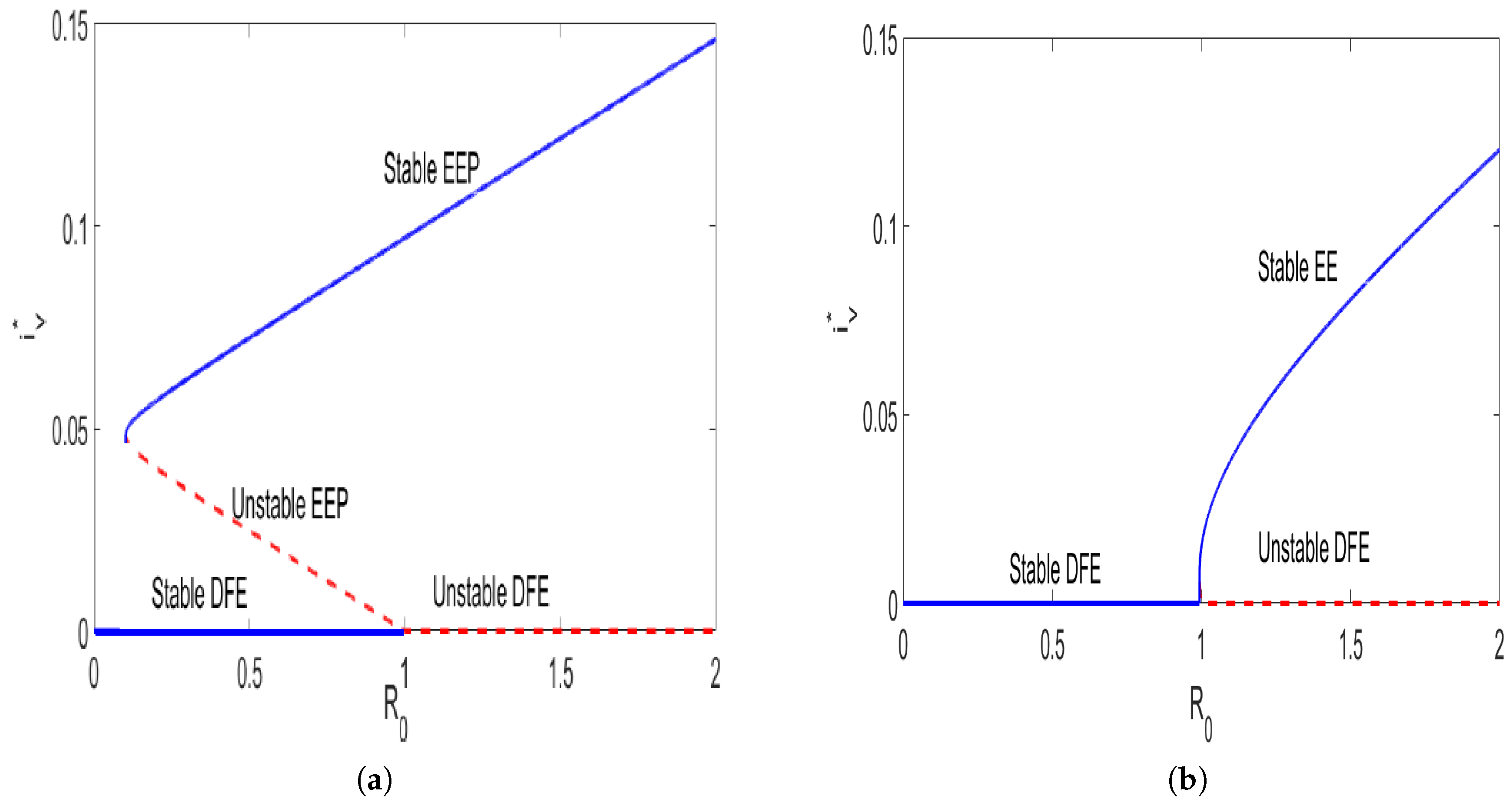
2.4. Existence and Uniqueness of the Endemic Equilibria

Let ${\mathcal{E}}^{*}=(s_h^{*},i_h^{*},i_a^{*},r_a^{*},i_v^{*})$ be any endemic equilibrium of model (3). Solving the first four equations of system (3) in terms of $i_v^{*}$ one gets the following results:

$$\left\{\begin{array}{ccc}{\displaystyle s_h^{*}}\hfill & =\hfill & {\displaystyle \frac{m_2{m}_3}{m_2(m_1+{\gamma }_h)+{\beta }_{vh}{i}_v^{*}(m_2+{\gamma }_h)},i_h^{*}=\frac{{\beta }_{vh}{i}_v^{*}{m}_3}{m_2(m_1+{\gamma }_h)+{\beta }_{vh}{i}_v^{*}(m_2+{\gamma }_h)},}\hfill \\ {\displaystyle i_a^{*}}\hfill & =\hfill & {\displaystyle \frac{{\beta }_{va}{i}_v^{*}{m}_5}{m_4{m}_5+{\beta }_{va}{i}_v^{*}({\alpha }_a+m_5)},r_a^{*}=\frac{{\beta }_{va}{i}_v^{*}{\alpha }_a}{m_4{m}_5+{\beta }_{va}{i}_v^{*}({\alpha }_a+m_5)},}\hfill \end{array}\right.$$

with

$$\begin{array}{ccc}{m}_1\hfill & =& ({\mu }_h+{\theta }_h),m_2=(\mu +{\alpha }_h),m_3=({\mu }_h+{\gamma }_h),\hfill \\ m_4\hfill & =& ({\mu }_a+{\alpha }_a),m_5=({\mu }_a+{\gamma }_a).\hfill \end{array}$$

Substituting $i_h^{*}$ and $i_a^{*}$ into the last equation of (3) yields

$$\begin{array}{c}g\left(i_v^{*}\right)=A{\left(i_v^{*}\right)}^2+B{i}_v^{*}+C=0,\hfill \end{array}$$

(4)

where

$$\begin{array}{ccc}A\hfill & =& {\beta }_{vh}{\beta }_{va}[m_2({\alpha }_a{\mu }_v+m_5({\mu }_v+{\beta }_{av}))+{\beta }_{hv}{m}_3({\alpha }_a+m_5)+{\gamma }_h({\alpha }_a{\mu }_v+m_5({\mu }_v+{\beta }_{av}))],\hfill \\ B\hfill & =& {\beta }_{va}(m_1{m}_2({\mu }_v{\alpha }_a+m_5({\mu }_v+{\beta }_{av}))-{\beta }_{vh}{\beta }_{hv}{m}_3({\beta }_{va}({\alpha }_a+m_5)-m_4{m}_5)\hfill \\ & & -{\beta }_{vh}{m}_5{\gamma }_h({\beta }_{av}{\beta }_{va}-m_4{\mu }_v)+m_2(m_4{m}_5{\mu }_v{\beta }_{vh}+{\beta }_{va}({\mu }_v{\alpha }_a{\gamma }_h+m_5({\mu }_v{\gamma }_h+{\beta }_{av}({\gamma }_h-{\beta }_{vh})))),\hfill \\ & & -{\beta }_{vh}({\beta }_{hv}+{\beta }_{av})\left)\right)]+{\alpha }_h{m}_4{\beta }_{vh}(m_3({\mu }_v+{\delta }_v)-{\beta }_{va}{\beta }_{av}),\hfill \\ C\hfill & =& m_2{m}_4{m}_5{\mu }_v(m_1+{\gamma }_h)(1-{\mathcal{R}}_0^2).\hfill \end{array}$$

Based on the fact that all parameters in (3) are positive for $t\ge 0$, it follows from (4) that $A>0$. Furthermore, $C>0$ when ${\mathcal{R}}_0<1$. Therefore the number of possible positive real roots the polynomial (4) hinges on the signs of B and C. By applying the Descartes rule of signs on the quadratic equation $g\left(i_v^{*}\right)=0$, given in (4), we list the various possibilities for the roots of $g\left(i_v^{*}\right)$ in

Table 2. Number of possible positive real roots of $g\left(i_v^{*}\right)$ given in (4) for ${\mathcal{R}}_0<1$ and ${\mathcal{R}}_0>1$.

Case	A	B	C	Reproduction Number	No. of Sign Changes	No. of Possible Positive Real Roots
1	+	+	+	${\mathcal{R}}_0<1$	0	0
2	+	+	-	${\mathcal{R}}_0>1$	1	1
3	+	-	+	${\mathcal{R}}_0<1$	2	0,2
4	+	-	-	${\mathcal{R}}_0>1$	1	1

.

Based on the different possibilities presented in Table 2, we have the following results:

Theorem 2.

The model (3) admits:

(i) 

A unique endemic equilibrium ${\mathcal{E}}^{*}$ if ${\mathcal{R}}_0>1$ and cases 2 and 4 are satisfied;

(ii) 

More than one endemic equilibrium if ${\mathcal{R}}_0<1$ and part of case 3 holds;

(iii) 

No endemic equilibrium if ${\mathcal{R}}_0<1$, and cases 1 and part of case 3 are satisfied.

The occurrence of a backward bifurcation, where a stable disease-free equilibrium coexists with a stable endemic equilibrium, is a common phenomenon in vector-borne disease models—more often for model that incorporates disease-related death for the host [33]. Since model (3) has disease-related death for both animals and humans, in what follows we check if the model does indeed have a backward bifurcation. To investigate the possibility of this phenomenon, the discriminant of Equation (4) is set to zero ($B^2-4AC=0)$ and solved to determine the critical value of ${\mathcal{R}}_0$, denoted by ${\mathcal{R}}_{0c}$, as follows:

$$\begin{array}{c}{\mathcal{R}}_{0c}=\sqrt{1-\frac{B^2}{4A{m}_2{m}_4{m}_5{m}_6(m_1+{\gamma }_h)}}.\hfill \end{array}$$

(5)

Numerical illustration in Figure 1 were performed using data in Table 1 in order to demonstrate that if ${\mathcal{R}}_0<1$ model (3) exhibits a backward bifurcation and for ${\mathcal{R}}_0>1$ the model admits a forward bifurcation. We have also noted that the switch occurs when ${\theta }_h=0.764$, thus, ${\mathcal{R}}_{0c}=0.139<1.$ Overall, we conclude that the model has two endemic equilibria—one stable and the other unstable. As ${\mathcal{R}}_0$ approaches one, the unstable endemic equilibrium loses its nature and coalesces with the disease-free equilibrium at ${\mathcal{R}}_0=1.$

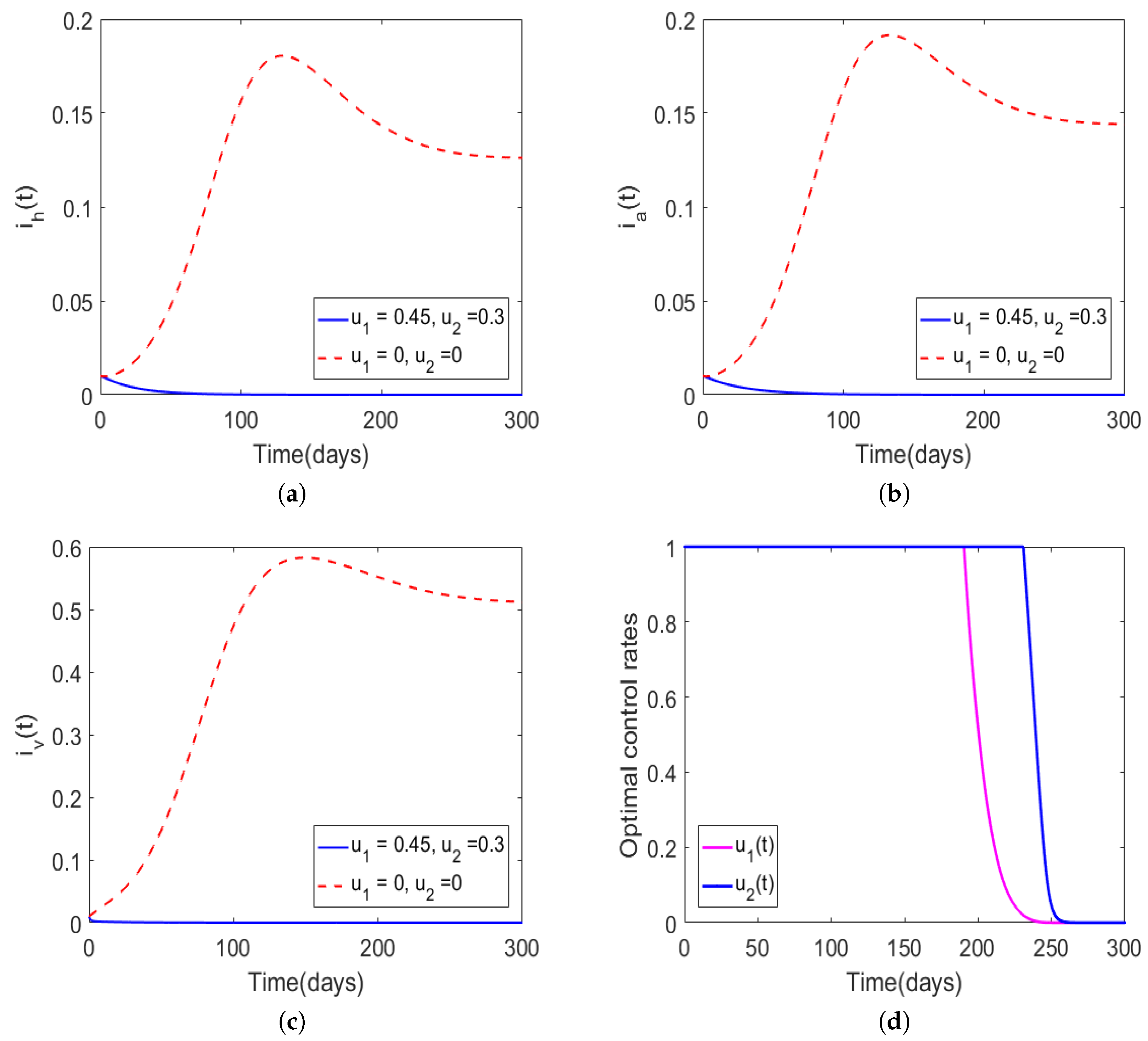
2.5. Optimal Control

Although there is no vaccine or drug for prophylaxis against African trypanosomiasis, there are other preventative and treatment options. HAT preventative strategies aim to minimize contact between the hosts and vectors. Humans can minimize contact with the tsetse vector by: using insect repellents, avoiding bushy areas, and wearing long-sleeved garments of medium-weight material in neutral colors that blend with the background environment. Spraying domesticated animals with insecticides also minimizes contact between the vector and the animals. Drugs can also be used to treat infected host species. Above all, the success of both preventative and corrective mechanisms revolves around the level of awareness of the human population. Through awareness, humans can effectively reduce contact between the vectors and multiple species. Thus, in this section we explore the impact of time-dependent awareness campaigns and time-dependent insecticides use on the dynamics of Trypanosoma brucei rhodesiense.

In order to investigate the effects of the aforementioned optimal control strategy, we reformulate system (3) to include time-dependent media campaigns $u_1\left(t\right)$ and insecticide use $u_2\left(t\right)$. The controls, $u_1\left(t\right)$ and $u_2\left(t\right)$, are functions of time and will be assigned reasonable upper and lower bounds. Furthermore, we also introduce an additional constant parameter $\delta$ to account for tsetse insecticide-induced mortality at the maximum possible rate. Using the same variable and parameter names as in (3), the system of differential equations describing our model with controls is:

$$\left\{\begin{array}{cc}{s}_h^{\prime }\left(t\right)\hfill & ={\mu }_h-{\beta }_{vh}{i}_v\left(t\right)s_h\left(t\right)-({\mu }_h+u_1\left(t\right){\theta }_h)s_h\left(t\right)+{\gamma }_h(1-s_h\left(t\right)-i_h\left(t\right)),\hfill \\ i_h^{\prime }\left(t\right)\hfill & ={\beta }_{vh}{i}_v\left(t\right)s_h\left(t\right)-({\mu }_h+{\alpha }_h+d_h)i_h\left(t\right),\hfill \\ i_a^{\prime }\left(t\right)\hfill & ={\beta }_{va}{i}_v\left(t\right)(1-i_a\left(t\right)-r_a\left(t\right))-({\mu }_a+{\alpha }_a+d_a)i_a\left(t\right),\hfill \\ r_a^{\prime }\left(t\right)\hfill & ={\alpha }_a\left(t\right)i_a\left(t\right)-({\mu }_a+{\gamma }_a)r_a\left(t\right),\hfill \\ i_v^{\prime }\left(t\right)\hfill & =\left({\beta }_{hv}{i}_h\left(t\right)+{\beta }_{av}{i}_a\left(t\right)\right)(1-i_v\left(t\right))-({\mu }_v+u_2\left(t\right){\delta }_v)i_v\left(t\right).\hfill \end{array}\right.$$

(6)

A successful control is one that minimizes the proportion of infected host (humans and animal), while minimizing the costs associated with these efforts. Thus, our goal is to find a control pair $(u_1^{*},u_2^{*})$ that minimizes the proportion of infected host over a finite time interval $[0,t_f]$ at minimal cost. Mathematically, the objective functional is proposed as follows:

$$\begin{array}{c}J(u_1\left(t\right),u_2\left(t\right))={\int }_0^{t_f}\left(c_1{i}_h\left(t\right)+c_2{i}_a\left(t\right)+\frac{w_1}{2}{u}_1^2\left(t\right)+\frac{w_2}{2}{u}_2^2\left(t\right)\right)dt,\hfill \end{array}$$

(7)

subject to the constraints of the ODEs in system (6) and where $c_1,c_2,w_1$ and $w_2$ are positive constants also known as the balancing coefficients and their goal is to transfer the integral into monetary quantity over a finite time interval $[0,t_f].$ In (7) control efforts are assumed to be nonlinear-quadratic, since a quadratic structure in the control has mathematical advantages, such as: if the control set is compact and convex it follows that the Hamiltonian attains its minimum over the control set at a unique point [34]. The optimal control problem becomes seeking an optimal function, $(u_1^{*}\left(t\right),u_2^{*}\left(t\right))$, such that

$$\begin{array}{c}J(u_1^{*}\left(t\right),u_2^{*}\left(t\right))=\underset{(u_1,u_2)\in U}{inf}J(u_1\left(t\right),u_2\left(t\right))\hfill \end{array}$$

(8)

for the admissible set $U=\{(u_1\left(t\right),u_2\left(t\right))\in {\left(L^{\infty }(0,t_f)\right)}^2:0\le u_i\left(t\right)\le q_i;q_i\in {\mathbb{R}}^{+},i=1,2\}$, where $q_i$ denotes the upper bound of the controls.

2.5.1. Existence and Uniqueness Results

The following theorem proves the existence of the optimal controls.

Theorem 3.

There exists an optimal control pair $(u_1^{*},u_2^{*})\in U$ with corresponding non-negative states $(s_h^{*},i_h^{*},i_a^{*},r_a^{*},i_v^{*})$ that minimizes the objective functional $J(u_1\left(t\right),u_2\left(t\right))$.

Proof. 

The uniform boundedness and the positivity of the controls and state variables over the finite interval $[0,t_f]$ imply that there exists a minimizing sequence $(u_1^n\left(t\right),u_2^n\left(t\right))$ such that

$$\underset{n\to \infty }{lim}J(u_1^n\left(t\right),u_2^n\left(t\right))=\underset{(u_1\left(t\right),u_2\left(t\right))\in U}{inf}J(u_1\left(t\right),u_2\left(t\right)).$$

Let the corresponding sequence of state variables be denoted by $(s_h,i_h,i_a,r_a,i_v).$ Furthermore, the boundedness of all the state and control variables implies that all the derivatives of the state variables are also bounded. Hence, it follows that all state variables are Lipschitz continuous with the same Lipschitz constant. Thus, the sequence $(s_h,i_h,i_a,r_a,i_v)$ is uniformly equicontinuous in $[0,t_f]$. By the Arzela–Ascoli Theorem [35], it follows that the state sequence has a subsequence that converges uniformly to $(s_h,i_h,i_a,r_a,i_v)$ in $[0,t_f]$.

In addition, we can establish that the control sequence $u^n=(u_1^n\left(t\right),u_2^n\left(t\right))$ has a subsequence that converges weakly in $L^2(0,t_f).$ Let $(u_1^{*},u_2^{*})\in U$ be such that $u_i^n\rightharpoonup u_i^{*}$ weakly in $L^2(0,t_f)$ for $i=1,2.$ Applying the lower semi-continuity of norms in weak $L^2$, one gets

$$\parallel u_i^{*}{\parallel }_{L^2}^2\le \underset{n\to \infty }{lim}inf{\parallel u_i^n\left(t\right)\parallel }_{L^2}^2,\mathrm{for}i=1,2.$$

Hence,

$$\begin{array}{ccc}J(u_1^{*},u_2^{*})\hfill & \le & \underset{n\to \infty }{lim}{\int }_0^{t_f}\left(c_1{i}_h^n\left(t\right)+c_2{i}_a^n\left(t\right)+\frac{w_1}{2}{u}_1^n\left(t\right)+\frac{w_2}{2}{u}_2^n\left(t\right)\right)dt\hfill \\ & =& \underset{n\to \infty }{lim}J(u_1^n,u_2^n).\hfill \end{array}$$

Therefore we conclude that there exists a pair of controls $(u_1^{*},u_2^{*})$ that minimizes the objective functional $J(u_1\left(t\right),u_2\left(t\right)).$ □

In what follows we characterize the optimal control pair by utilizing Pontryagin’s Maximum Principle [36].

2.5.2. Characterization of an Optimal Control Pair

Since there exists an optimal control pair for minimizing the functional (7) subject to the constraints of the ODEs in system (6), we now apply Pontryagin’s Maximum Principle [36] to derive the necessary conditions for this optimal control pair. Thus, system (6) is converted into an equivalent problem, namely, the problem of minimizing the Hamiltonian $H\left(t\right)$ given by:

$$\begin{array}{ccc}H\left(t\right)\hfill & =& c_1{i}_h\left(t\right)+c_2{i}_a\left(t\right)+\frac{w_1}{2}{u}_1^2\left(t\right)+\frac{w_2}{2}{u}_2^2\left(t\right)\hfill \\ & & +{\lambda }_1\left(t\right)\left[{\mu }_h-{\beta }_{vh}{i}_v\left(t\right)s_h\left(t\right)-({\mu }_h+u_1\left(t\right){\theta }_h)s_h\left(t\right)+{\gamma }_h(1-s_h\left(t\right)-i_h\left(t\right))\right]\hfill \\ & & +{\lambda }_2\left(t\right)\left[{\beta }_{vh}{i}_v\left(t\right)s_h\left(t\right)-({\mu }_h+{\alpha }_h+d_h)i_h\left(t\right)\right]\hfill \\ & & +{\lambda }_3\left(t\right)\left[{\beta }_{va}{i}_v\left(t\right)(1-i_a\left(t\right)-r_a\left(t\right))-({\mu }_a+{\alpha }_a+d_a)i_a\left(t\right)\right]\hfill \\ & & +{\lambda }_4\left(t\right)\left[{\alpha }_a{i}_a\left(t\right)-({\mu }_a+{\gamma }_a)r_a\left(t\right)\right]\hfill \\ & & +{\lambda }_5\left(t\right)\left[\left({\beta }_{hv}{i}_h\left(t\right)+{\beta }_{av}{i}_a\left(t\right)\right)(1-i_v\left(t\right))-({\mu }_v+u_2\left(t\right){\delta }_v)i_v\left(t\right)\right].\hfill \end{array}$$

Given an optimal control pair $(u_1^{*},u_2^{*})$ and solutions $(s_h,i_h,i_a,r_a,i_v)$, of the corresponding states system (6) there exist adjoint functions ${\lambda }_i\left(t\right)$, ($i=1,2,3,4,5$) [37], satisfying

$$\begin{array}{ccc}{\lambda }_1^{\prime }\left(t\right)\hfill & =& {\lambda }_1\left(t\right)({\mu }_h+u_1\left(t\right){\theta }_h+{\gamma }_h+{\beta }_{vh}{i}_v\left(t\right))-{\lambda }_2\left(t\right){\beta }_{vh}{i}_v\left(t\right),\hfill \\ {\lambda }_2^{\prime }\left(t\right)\hfill & =& -c_1+{\lambda }_1\left(t\right){\gamma }_h+{\lambda }_2\left(t\right)({\mu }_h+{\alpha }_h+d_h)-{\lambda }_5\left(t\right){\beta }_{hv}(1-i_h\left(t\right)),\hfill \\ {\lambda }_3^{\prime }\left(t\right)\hfill & =& -c_2+{\lambda }_3\left(t\right)({\mu }_a+{\alpha }_a+{\beta }_{va}{i}_v\left(t\right))-{\lambda }_4\left(t\right){\alpha }_a-{\lambda }_5\left(t\right){\beta }_{av}(1-i_v\left(t\right)),\hfill \\ {\lambda }_4^{\prime }\left(t\right)\hfill & =& {\lambda }_3\left(t\right){\beta }_{va}{i}_v\left(t\right)+{\lambda }_4\left(t\right)({\mu }_a+{\gamma }_a),\hfill \\ {\lambda }_5^{\prime }\left(t\right)\hfill & =& ({\lambda }_1\left(t\right)-{\lambda }_2\left(t\right)){\beta }_{vh}-{\lambda }_3\left(t\right){\beta }_{va}(1-i_a\left(t\right)-r_a\left(t\right))+{\lambda }_5\left(t\right)({\mu }_v+u_2\left(t\right)\delta +{\beta }_{hv}{i}_h\left(t\right)+{\beta }_{av}{i}_a\left(t\right)),\hfill \end{array}$$

with transversality conditions ${\lambda }_j\left(t_f\right)=0$ for $j=1,2,3,4,5$. Furthermore, the optimal solutions of the Hamiltonian are determined by taking the partial derivatives of the function $H\left(t\right)$ in (9) with respect to control functions $u_1$ and $u_2$, followed by setting the resultant equation to zero and then solving for $u_1^{*}$ and $u_2^{*}$, as follows:

$$\begin{array}{ccc}{\displaystyle \frac{\partial H}{\partial u_1}}\hfill & =& {\displaystyle u_1^{*}{w}_1-{\lambda }_1{\theta }_h{s}_h,\mathrm{and}\frac{\partial H}{\partial u_2}=u_2^{*}{w}_2-{\lambda }_5{\delta }_v{i}_v.}\hfill \end{array}$$

(9)

Setting (9) to zero and solving for $u_1^{*}$ and $u_2^{*}$, one gets

$$\begin{array}{c}{u}_1^{*}=\frac{{\theta }_h{s}_h{\lambda }_1}{w_1},u_2^{*}=\frac{{\delta }_v{i}_v{\lambda }_5}{w_2}.\hfill \end{array}$$

Using the standard arguments and the bounds for the controls, we obtain the characterization of this optimal pair as follows:

$$\begin{array}{ccc}{u}_1\left(t\right)\hfill & =& {\displaystyle min\left\{q_1,max\left(0,\frac{{\theta }_h{s}_h{\lambda }_1}{w_1}\right)\right\},u_2\left(t\right)=min\left\{q_2,max\left(0,\frac{{\delta }_v{i}_v\left(t\right){\lambda }_5}{w_2}\right)\right\}.}\hfill \end{array}$$

In what follows, we numerically investigate the impact of awareness campaigns and insecticide use using the forward–backward sweep algorithm as outlined in [37]. We set $c_1=2c_2$, implying that the minimization of the infected humans has more importance/weight compared to that of infected animals. Furthermore, we assumed that the intensity of implementation of awareness campaigns was always higher than that of insecticide use since excessive insecticide use is associated with ecological side effects, hence their usage should always be kept as low as possible [38]. Thus, $u_1$ was assumed to be greater than $u_2$. It was also hypothetically assumed that the cost of insecticide use was higher than awareness campaign costs. The initial population levels were set as follows: $s_h=0.99$, $i_h=0.01$, $r_h=0$, $i_a=0.01$, $r_a=0$, $i_v=0.01$, that is, each species comprised 1% of the infected population and no recoveries for the hosts. Also, we assumed that ${\delta }_v=1$ per day. The total number of new infections generated within the human population in the presence and absence of optimal control is:

$$T_h={\int }_0^{t_f}\left({\beta }_{vh}{i}_v\left(t\right)N_v{s}_v\left(t\right)N_h\right)dt.$$

Similarly, the total number of new infections generated within the animal population in the presence and absence of optimal control is:

$$T_a={\int }_0^{t_f}\left({\beta }_{va}{i}_v\left(t\right)N_v(1-i_a\left(t\right)-r_a\left(t\right))N_a\right)dt,$$

where $N_h$, $N_a$ and $N_v$ are constants and are equivalent to 100,000, 10,000 and 50,000, respectively. Figure 2 shows the dynamics of Trypanosoma brucei rhodesiense with $u_1=0.45$ and $u_2=0.3.$ We can observe that in the presence of optimal intervention strategies, the proportion of infectious hosts and vectors would never exceed the initial assumed population levels (1%). In particular, in the presence of optimal awareness and insecticides use, the population levels for the hosts and vectors converged to the disease-free equilibrium suggesting that the aforementioned optimal control mechanisms could lead to disease eradication. Precisely, we noted that in the presence of optimal control, the total numbers of new infections for the human and animal populations generated over 300 days were $2.5635\times {10}^5$, $9.7\times {10}^4$, respectively, and the total cost was $J=6.5028\times {10}^4.$ However, in the absence of optimal controls (i.e., $u_1=u_2=0$), one can observe that the disease persisted. In Figure 2d, we observe that the control profiles of $u_1$ and $u_2$ started at the maximum, and they remained there for approximately 200 and 250 days, respectively, suggesting that awareness campaigns could essentially be ceased after 200 days of implementation while insecticides use needed to be maintained at maximum strength for an additional 50 days.

Figure 3 shows the optimal control profiles for $u_1$ and $u_2$ when the upper bounds for these controls were less than unity (i.e., $q_1=0.5$ and $q_2=0.3$), with initial guesses of the controls set to $u_1=0.45$ and $u_2=0.3$. We again see that both $u_1$ and $u_2$ started from their maxima, and they stayed at the maximum strength for much longer periods of time than the previous case (compared to Figure 2), due to the reduced intensity bounds. When the upper bounds of the controls were reduced, the population levels for all the infected species would converge to zero within the defined time interval, $t_f=300$ (the figures were omitted since their behavior was analogous to that of Figure 2). We also note that by reducing the bounds for the controls, the total cost $J(=5.3582\times {10}^4)$ was reduced $17.6$%, compared to that of Figure 2.

Numerical results in Figure 4 show the dynamics of Trypanosoma brucei rhodesiense disease when the population of infectious vectors was 3% and the hosts’ infectious populations were 1% each, and the controls had the following bounds set to $q_1=0.5$, $q_2=0.3$ and the initial guesses of the controls were set to $u_1=0.45$ and $u_2=0.3$. Again, we can note that the population levels would converge to the disease-free equilibrium in the presence of optimal control, whereas in the absence of optimal control the disease persisted. The total numbers of new infections for the human and animal populations generated over 300 days were $3.7167\times {10}^5$ and $1.1232\times {10}^4$, respectively, and the total cost was $J=5.4726\times {10}^4.$ In Figure 4d, we note that the control profiles for $u_1$ and $u_2$ exhibited a similar behavior to the one illustrated in Figure 3. Comparing the results in Figure 2 and Figure 4, one can observe that even if the total number of new infections for the hosts increased due to an increase in the infectious vector population, the total cost would still be lower by approximately 15.8%.

Next, we determined the impact of extremely low-intensity controls on Trypanosoma brucei rhodesiense disease dynamics (Figure 5). We set the initial guess for the controls to $u_1=0.15$, $u_2=0.01$, and the upper bounds of the controls were set to $q_1=0.15$ and $q_2=0.01.$ Furthermore, the we set the initial population levels and the weight constants to $i_h=i_a=0.01$, $i_v=0.03$, $r_h=r_a=0$, $s_h=1-i_h-r_h$, $s_a=1-i_a-r_a$, $s_v=1-i_v$, $w_1=10$, and $w_2=100$. Although the Figures of the population level effects are not displayed, since their behavior was similar to that of Figure 4, we can report that in the presence of optimal control the infected population levels would converge to the disease-free equilibrium and the reverse would occur in the absence of optimal control. The total numbers of new infections for the human and animal populations generated over 300 days were $4.8695\times {10}^5$ and $1.2764\times {10}^4$, respectively, and the total cost was $J=5.4519\times {10}^4.$ From these simulation results, we see that for effective disease management the control profiles would have to be maintained at their maximum intensity for most of the implementation period. Despite the fact that we considered the insecticide control as more expensive than the awareness control, we note that this control had to be maintained at its maximum intensity for a slightly more time even after the awareness control was dropped.

Next, we determined the number of new infections averted by the implementation of optimal control. This was determined by taking the difference between the total numbers of new infections observed in the absence of optimal control and those recorded when optimal control was implemented. The results are displayed in

Table 3. Infection reduction due to the implementation of optimal control.

Case	Host	Total Number of New Infections Observed with Optimal Control	Infections Averted Due to Implementation of Optimal Control
Figure 2	Human population	$2.5635\times {10}^5$	$1.0097\times {10}^7$
	Animal population	$9.7000\times {10}^4$	$7.7141\times {10}^7$
Figure 4	Human population	$3.7197\times {10}^5$	$1.04943\times {10}^7$
	Animal population	$1.1232\times {10}^4$	$7.7226\times {10}^7$
Figure 5	Human population	$4.8695\times {10}^5$	$1.03791\times {10}^7$
	Animal population	$1.2764\times {10}^4$	$7.7224\times {10}^7$

. The total numbers of new infections generated in the human and animal populations in the absence of optimal control were $1.0866\times {10}^7$ and $7.7237\times {10}^7$, respectively.

From Table 3, we see that the number of infections averted was extremely high even when the intensity of the optimal controls was low, and this clearly shows the strength of optimal control strategies in minimizing the spread of the disease.

3. Concluding Remarks

In this paper, a mathematical model for Trypanosoma brucei rhodesiense transmission was proposed and analyzed. The framework incorporated three species: human, animal, and vector populations. In addition, the impact of optimal awareness campaigns and insecticides use to minimize the populations of infected humans and animals at minimal cost was investigated. The preliminary analysis of the proposed model revealed that the system always had a unique and positively bounded solution for all $t\ge 0.$ Qualitative analysis of the model showed that it admitted a backward bifurcation generated by awareness campaigns. In particular, the backward bifurcation occurred whenever the reproduction number was less than unity and the awareness campaign rate, whereas for ${\mathcal{R}}_0>1$ the model exhibited a forward bifurcation.

Meanwhile, the basic Trypanosoma brucei rhodesiense model was extended to investigate the impact of optimal awareness and insecticide use to minimize the population of infected humans and animals at minimal cost. Analysis of the optimal model was done with the population levels for the hosts (humans and animals) fixed at 1% while the vector population was varied from 1% to 3%. In addition, in the entire analysis, the intensity of awareness campaigns was assumed to be higher than that of insecticide use since the excessive use of insecticides has some residual effects. Although the insecticide intensity was assumed to be low, the associated cost for this control was regarded to be higher than that of awareness campaigns. Furthermore, the minimization of the infected humans was considered to be more important than that of infected animals. Optimal control results indicate that optimal control awareness campaigns and insecticides use have the potential to eliminate the disease in the community, whereas in the absence of optimal control the disease may not be reduced to levels close to zero. We observed that when the bounds of the control were high the associated costs were also high, and the reverse was true. In particular, we observed that reducing the upper bound of $u_1$ from 1 to 0.5 and $u_2$ from 1 to 0.3 could lead to a reduction in costs by 17.6%. Overall, the study demonstrated that optimal awareness and insecticide use have the potential to reduce the population levels of infected species to levels close to zero, and for this to be attained the insecticide control has to be implemented for a slightly longer period compared to the awareness control. In addition, the results from this study suggest that the use of insecticides to control the spread of the disease could have more impact. The strength of using insecticides to control the transmission dynamics of the disease was also noted in the work of Hagrove et al. [12]. Utilizing a mathematical model, Hagrove et al. [12] demonstrated that using insecticides to treat cattle would have a greater impact on controlling the transmission of the disease compared treatment of cattle with drugs.

This work is not exhaustive. In future we hope to explore the dynamics of the disease by using a model with varying total populations for the species, since the constant population approach used in this study does not adequately capture the dynamics of the disease for long periods of time. We will also extend this work to explore the effects of climatic conditions on the long-term dynamics of the disease.

References

1. World Health Organization. Human African trypanosomiasis (sleeping sickness): Epidemiological update. Wkly. Epidemiol. Rec. 2018, 81, 71–80. [Google Scholar]
2. Franco, J.R.; Simarro, P.P.; Diarra, A.; Jannin, J.G. Epidemiology of human African trypanosomiasis. Clin. Epidemiol. 2014, 6, 257–275. [Google Scholar]
3. Lutumba, P.; Makieya, E.; Shaw, A.; Meheus, F.; Boelaert, M. Human African Trypanosomiasis in a Rural Community, Democratic Republic of Congo. Emerging Infectious Diseases. Available online: www.cdc.gov/eid (accessed on 8 May 2012).
4. Kermack, W.O.; McKendrick, A.G. A contribution to the mathematical theory of epidemics. Proc. Soc. Lond. Ser. Math. Phys. Eng. Sci. 1927, 115, 700–721. [Google Scholar] [CrossRef] [Green Version]
5. Mushayabasa, S.; Posny, D.; Wang, J. Modeling the intrinsic dynamics of foot–and–mouth disease. Math. Biosci. Eng. 2016, 13, 425–442. [Google Scholar] [CrossRef] [PubMed]
6. Okosun, K.O.; Ouifki, R.; Marcus, N. Optimal control analysis of a malaria disease transmission model that includes treatment and vaccination with waning immunity. BioSystems 2011, 106, 136–145. [Google Scholar] [CrossRef] [PubMed]
7. Cai, L.; Li, X.; Tuncer, N.; Martcheva, M.; Lashari, A. Optimal control of a malaria model with asymptomatic class and superinfection. Math. Biosci. 2017, 288, 94–108. [Google Scholar] [CrossRef] [PubMed]
8. Kalinda, C.; Mushayabasa, S.; Chimbari, J.M.; Mukaratirwa, S. Optimal control applied to a temperature dependent schistosomiasis model. Biosystems 2017, 175, 47–56. [Google Scholar] [CrossRef]
9. Lolika, O.P.; Mushayabasa, S. On the role of short-term animal movements on the persistence of brucellosis. Mathematics 2018, 6, 154. [Google Scholar] [CrossRef]
10. Chitnis, N.; Hyman, J.M.; Cushing, J.M. Determining important parameters in the spread of malaria through the sensitivity analysis of a mathematical model. Bull. Math. Biol. 2018, 70, 1272–1296. [Google Scholar] [CrossRef]
11. Mushayabasa, S.; Bhunu, C.P. Modelling the impact of early therapy for latent tuberculosis patients and its optimal control analysis. J. Biol. Phys. 2013, 39, 723–747. [Google Scholar] [CrossRef]
12. Hargrove, J.W.; Ouifki, R.; Kajunguri, D.; Vale, G.A.; Torr, S.J. Modeling the control of trypanosomiasis using trypanocides or insecticide-treated livestock. PLoS Negl. Trop. Dis. 2012, 6, e1615. [Google Scholar] [CrossRef] [PubMed]
13. Kajunguri, D.; Hargrove, J.W.; Ouifki, R.; Mugisha, J.Y.T.; Coleman, P.G.; Welburn, S.C. Modelling the use of insecticide-treated cattle to control tsetse and Trypanosoma brucei rhodiense in a multi-host population. Bull. Math. Biol. 2014, 76, 673–696. [Google Scholar] [CrossRef] [PubMed]
14. Moore, S.; Shrestha, S.; Tomlinson, K.W.; Vuong, H. Predicting the effect of climate change on African trypanosomiasis: Integrating epidemiology with parasite and vector biology. J. R. Soc. Interface 2012, 9, 817–830. [Google Scholar] [CrossRef] [PubMed]
15. Peck, S.L.; Bouyer, J. Mathematical modeling, spatial complexity, and critical decisions in tsetse control. J. Econ. Entomol. 2012, 105, 1477–1486. [Google Scholar] [CrossRef]
16. Stone, C.M.; Chitnis, N. Implications of Heterogeneous Biting Exposure and Animal Hosts on Trypanosomiasis brucei gambiense Transmission and Control. Plos Comput. Biol. 2015, 11, e1004514. [Google Scholar] [CrossRef]
17. Artzrouni, M.; Gouteux, J.-P. Estimating tsetse population parameters: Application of a mathematical model with density-dependence. Med. Vet. Entomol. 2003, 17, 272–279. [Google Scholar] [CrossRef]
18. Artzrouni, M.; Gouteux, J.-P. A model of Gambian sleeping sickness with open vector populations. Math. Med. Biol. 2001, 18, 99–117. [Google Scholar] [CrossRef]
19. Artzrouni, M.; Gouteux, J.-P. Population dynamics of sleeping sickness: A microsimulation. Simul. Gaming 2001, 32, 215–227. [Google Scholar] [CrossRef]
20. Artzrouni, M.; Gouteux, J.-P. A compartmental model of sleeping sickness in Central Africa. J. Biol. Syst. 1996, 4, 459–477. [Google Scholar] [CrossRef]
21. Rogers, D.J. A general model for the African trypanosomiases. Parasitology 1998, 97, 193–212. [Google Scholar] [CrossRef]
22. Rock, K.S.; Ndeffo-Mbah, M.L.; Castaño, S. Assessing strategies against Gambiense sleeping sickness through mathematical modeling. Clin. Infect. Dis. 2018, 66, S286–S292. [Google Scholar] [CrossRef] [PubMed]
23. Ndondo, A.M.; Munganga, J.M.W.; Mwambakana, J.N.; Saad-Roy, M.C.; Van den Driessche, P.; Walo, O.R. Analysis of a model of gambiense sleeping sickness in human and cattle. J. Biol. Dyn. 2016, 10, 347–365. [Google Scholar] [CrossRef] [PubMed]
24. Gilbert, J.A.; Medlock, J.; Townsend, J.P.; Aksoy, S.; Mbah, M.N.; Galvani, A.P. Determinants of Human African Trypanosomiasis Elimination via Paratransgenesis. PLoS Negl. Trop. Dis. 2016, 10, e0004465. [Google Scholar] [CrossRef] [PubMed]
25. Rock, K.S.; Torr, S.J.; Lumbala, C.; Keeling, M.J. Predicting the impact of intervention strategies for sleeping sickness in two high-endemicity health zones of the Democratic Republic of Congo. PLoS Negl. Trop. Dis. 2017, 11, e0005162. [Google Scholar] [CrossRef] [PubMed]
26. Rock, K.S.; Torr, S.J.; Lumbala, C.; Keeling, M.J. Quantitative evaluation of the strategy to eliminate human African trypanosomiasis in the Democratic Republic of Congo. Parasit. Vectors 2015, 8, 532. [Google Scholar] [CrossRef] [Green Version]
27. Rock, K.S.; Stone, C.M.; Hastings, I.M.; Keeling, M.J.; Torr, S.J.; Chitnis, N. Mathematical models of human African trypanosomiasis epidemiology. Adv. Parasitol. 2015, 87, 53–133. [Google Scholar]
28. Randolph, W.; Viswanath, K. Lessons learned from public health mass media campaigns: marketing health in a crowded media world. Annu. Rev Public Health 2004, 25, 419–437. [Google Scholar] [CrossRef]
29. Apollonio, D.E.; Malone, R.E. Turning negative into positive: Public health mass media campaigns and negative advertising. Health Educ. Res. 2009, 24, 483–495. [Google Scholar] [CrossRef]
30. Noar, S.M. A 10-year retrospective of research in health mass media campaigns: where do we go from here? J. Health Commun. 2006, 11, 21–42. [Google Scholar] [CrossRef]
31. Leak, S.G.A. Tsetse vector population dynamics: ILRAD’s Requirements. In Modelling Vector-Borne and Other Parasitic Diseases; Hansen, J.W., Perry, B.D., Eds.; International Livestock Research Institute (ILRI): Nairobi, Kenya, 1994; p. 36. Available online: https://books.google.co.zw/books?isbn=9290552972 (accessed on 8 May 2012).
32. van den Driessche, P.; Watmough, J. Reproduction number and subthreshold endemic equilibria for compartment models of disease transmission. Math. Biosci. 2002, 180, 29–48. [Google Scholar] [CrossRef]
33. Gumel, A.B. Causes of backward bifurcation in some epidemiological models. J. Math. Anal. Appl. 2012, 395, 355–365. [Google Scholar] [CrossRef]
34. Silva, C.J.; Maurer, H.; Torres, D.F.M. Optimal control of a tuberculosis model with state and control delays. Math. Biosci. Eng. 2017, 14, 321–337. [Google Scholar] [CrossRef] [PubMed]
35. Lukes, D.L. Differential Equations: Classical to Controlled, Mathematics in Science and Engineering; Academic Press: New York, NY, USA, 1982; Volume 162. [Google Scholar]
36. Pontryagin, L.S.; Boltyanskii, V.T.; Gamkrelidze, R.V.; Mishcheuko, E.F. The Mathematical Theory of Optimal Processes; Wiley: New York, NY, USA, 1962. [Google Scholar]
37. Lenhart, S.; Workman, J.T. Optimal Control Applied to Biological Models; Chapman and Hall/CRC: London, UK, 2007. [Google Scholar]
38. Chávez, J.P.; Götz, T.; Siegmund, S.; Wijaya, K.P. Wijaya An SIR-Dengue transmission model with seasonal effects and impulsive control. Math. Biosci. 2017, 1, 29–39. [Google Scholar] [CrossRef] [PubMed]
Figure 1. Graphical results illustrating the possible bifurcations for model (3) for different values of awareness campaigns θ h . The figures were generated with parameter values taken from Table 1. Parameters different from those listed in Table 1 are β h v = β a v = 0.65 , β v h = β v a = 0.4 . In (a) we set θ h = 0.764 and in (b) θ h = 0.857 . For R 0 < 1 , the model has two endemic equilibria: one stable and the other unstable. As R 0 approaches one the unstable endemic equilibrium loses its nature and coalesces with the disease-free equilibrium at R 0 = 1 . Therefore, we conclude that the model admits a backward bifurcation whenever R 0 < 1 and a forward bifurcation for R 0 > 1 .
Mathematics 07 00971 g001
Figure 2. Simulations of model (6) with initial guess for the controls set to u 1 = 0.45 , u 2 = 0.3 and the bounds of the controls were q 1 = q 2 = 1 . The weight constants were set as w 1 = 10 , w 2 = 100 , and the model parameter values were adopted from Table 1. The solid curves in (ac) represent the proportion of infectious humans, infectious animals, and infectious tsetse vectors, respectively, in the presence of time-dependent control, and the dotted lines denote the absence of optimal control. The optimal control rates are shown in (d).
Mathematics 07 00971 g002
Figure 3. Numerical results illustrating the impact of the bounds for the control rates, with the initial guess for the controls set to u 1 = 0.45 and u 2 = 0.3 , and the bounds for these controls fixed to q 1 = 0.5 and q 2 = 0.3 . The remainder of the model parameter values are as in Table 1.
Mathematics 07 00971 g003
Figure 4. Simulations of model (6) with the initial guesses for the control set to u 1 = 0.45 , u 2 = 0.3 , and the bounds for the controls set to q 1 = 0.5 and q 2 = 0.3 . The rest of the model parameter values were adopted from Table 1. The solid curves in (ac) represent the proportion of infectious humans, infectious animals, and infectious tsetse vectors, respectively, in the presence of time-dependent control and the dotted lines denote the absence of optimal control. The optimal control rates are shown in (d).
Mathematics 07 00971 g004
Figure 5. Numerical results illustrating the impact of the bounds for the control rates. The initial guess for the control were u 1 = 0.15 and u 2 = 0.01 , the upper bounds of the controls were q 1 = 0.15 and q 2 = 0.01 . The weights constants were set to w 1 = 10 and w 2 = 100 and the rest of the model parameter values were as in Table 1.
Mathematics 07 00971 g005