A New X-Bar Control Chart for Using Neutrosophic Exponentially Weighted Moving Average


Abstract
1. Introduction
2. The Proposed NEWMA Statistics
3. The Proposed NEWMA X-Bar Control Chart
- Choose a random sample of size and compute statistics.
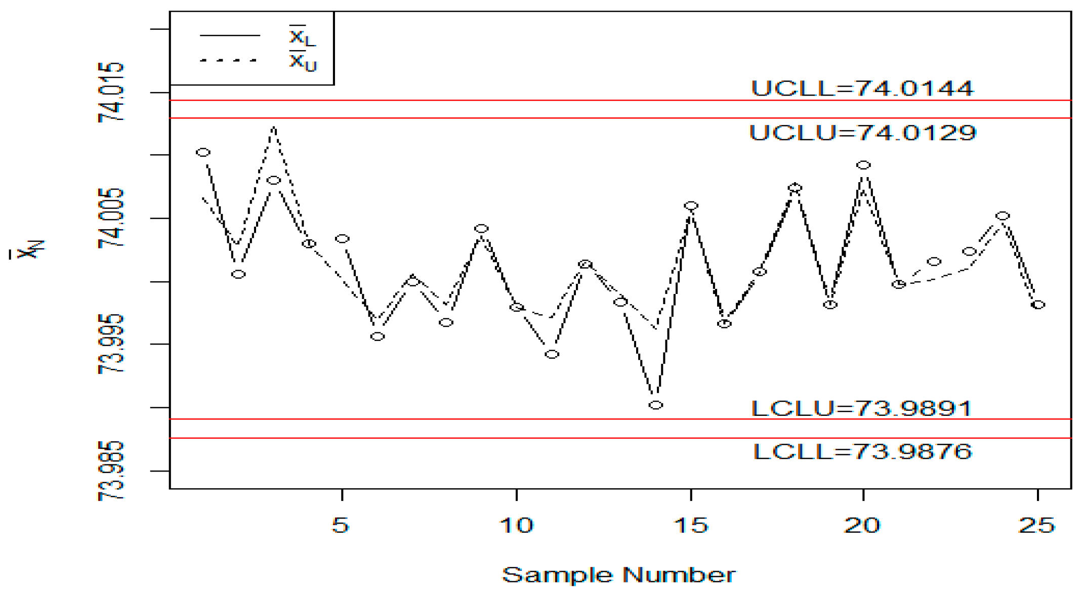
- Declare the process is an in-control state if ; otherwise, it is in an out-of-control state. Note here that and are the neutrosophic lower and upper control limits.
4. The Proposed Neutrosophic Monte Carlo Simulation (NMCS)
4.1. For In-Control State
4.2. For Shifted Process
5. Comparative Studies
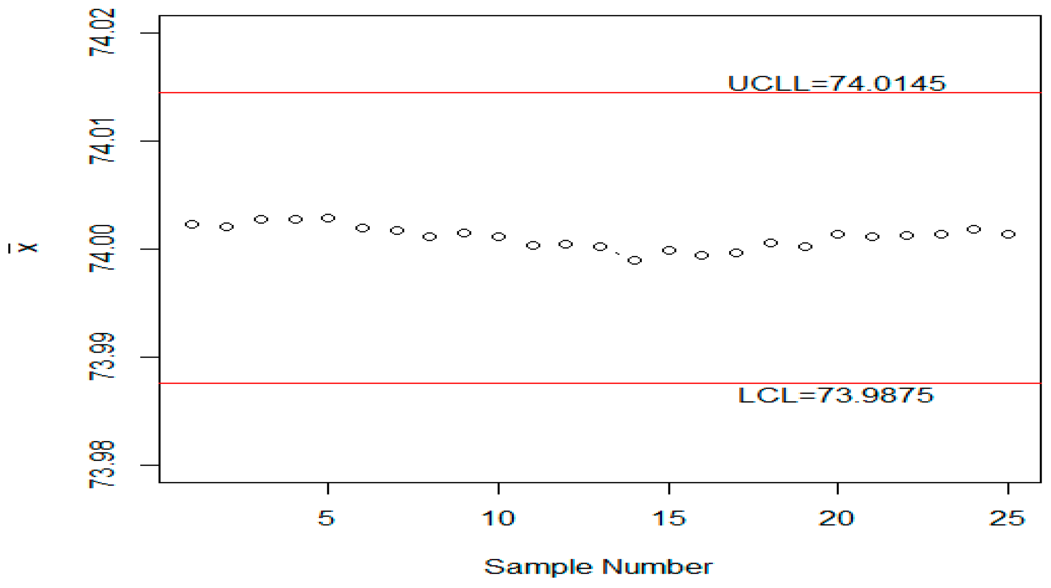
6. Application
7. Concluding Remarks
Author Contributions
Funding
Acknowledgments
Conflicts of Interest
References
- Senturk, S.; Erginel, N. Development of fuzzy X¯∼-R∼ and X¯∼-S∼ control charts using α-cuts. Inf. Sci. 2009, 179, 1542–1551. [Google Scholar] [CrossRef]
- Hart, M.K.; Lee, K.Y.; Hart, R.F.; Robertson, J.W. Application of Attribute Control Charts to Risk-Adjusted Data for Monitoring and Improving Health Care Performance. Qual. Manag. Healthc. 2003, 12, 5–19. [Google Scholar] [CrossRef]
- Bai, D.; Lee, K. Variable sampling interval X control charts with an improved switching rule. Int. J. Prod. Econ. 2002, 76, 189–199. [Google Scholar] [CrossRef]
- Castagliola, P.; Celano, G.; Fichera, S.; Nunnari, V. A variable sample size S2-EWMA control chart for monitoring the process variance. Int. J. Reliab. Qual. Saf. Eng. 2008, 15, 181–201. [Google Scholar] [CrossRef]
- Panthong, C.; Pongpullponsak, A. Non-Normality and the Fuzzy Theory for Variable Parameters Control Charts. Thai J. Math. 2016, 14, 203–213. [Google Scholar]
- Pereira, P.; Seghatchian, J.; Caldeira, B.; Xavier, S.; de Sousa, G. Statistical methods to the control of the production of blood components: Principles and control charts for variables. Transfus. Apher. Sci. 2018, 57, 132–142. [Google Scholar] [CrossRef]
- Roberts, S. Control chart tests based on geometric moving averages. Technometrics 1959, 1, 239–250. [Google Scholar] [CrossRef]
- Haq, A. An improved mean deviation exponentially weighted moving average control chart to monitor process dispersion under ranked set sampling. J. Stat. Comput. Simul. 2014, 84, 2011–2024. [Google Scholar] [CrossRef]
- Haq, A.; Brown, J.; Moltchanova, E. New exponentially weighted moving average control charts for monitoring process mean and process dispersion. Qual. Reliab. Eng. Int. 2015, 31, 877–901. [Google Scholar] [CrossRef]
- Haq, A.; Brown, J.; Moltchanova, E.; Al-Omari, A.I. Effect of measurement error on exponentially weighted moving average control charts under ranked set sampling schemes. J. Stat. Comput. Simul. 2015, 85, 1224–1246. [Google Scholar] [CrossRef]
- Abbasi, S.A.; Riaz, M.; Miller, A.; Ahmad, S.; Nazir, H.Z. EWMA dispersion control charts for normal and non-normal processes. Qual. Reliab. Eng. Int. 2015, 31, 1691–1704. [Google Scholar] [CrossRef]
- Abbasi, S.A. Exponentially weighted moving average chart and two-component measurement error. Qual. Reliab. Eng. Int. 2016, 32, 499–504. [Google Scholar] [CrossRef]
- Sanusi, R.A.; Riaz, M.; Adegoke, N.A.; Xie, M. An EWMA monitoring scheme with a single auxiliary variable for industrial processes. Comput. Ind. Eng. 2017, 114, 1–10. [Google Scholar] [CrossRef]
- Montgomery, D.C. Introduction to Statistical Quality Control; John Wiley & Sons: Hoboken, NJ, USA, 2007. [Google Scholar]
- Arshad, W.; Abbas, N.; Riaz, M.; Hussain, Z. Simultaneous use of runs rules and auxiliary information with exponentially weighted moving average control charts. Qual. Reliab. Eng. Int. 2017, 33, 323–336. [Google Scholar] [CrossRef]
- Adeoti, O.A. A new double exponentially weighted moving average control chart using repetitive sampling. Int. J. Qual. Reliab. Manag. 2018, 35, 387–404. [Google Scholar] [CrossRef]
- Adeoti, O.A.; Malela-Majika, J.-C. Double exponentially weighted moving average control chart with supplementary runs-rules. Qual. Technol. Quant. Manag. 2019, 1–24. [Google Scholar] [CrossRef]
- Hunter, J.S. The exponentially weighted moving average. J. Qual. Technol. 1986, 18, 203–210. [Google Scholar] [CrossRef]
- Lucas, J.M.; Saccucci, M.S. Exponentially weighted moving average control schemes: Properties and enhancements. Technometrics 1990, 32, 1–12. [Google Scholar] [CrossRef]
- Khademi, M.; Amirzadeh, V. Fuzzy rules for fuzzy $\overline{X}$ and $R$ control charts. Iran. J. Fuzzy Syst. 2014, 11, 55–66. [Google Scholar]
- Faraz, A.; Moghadam, M.B. Fuzzy control chart a better alternative for Shewhart average chart. Qual. Quant. 2007, 41, 375–385. [Google Scholar] [CrossRef]
- Zarandi, M.F.; Alaeddini, A.; Turksen, I. A hybrid fuzzy adaptive sampling–run rules for Shewhart control charts. Inf. Sci. 2008, 178, 1152–1170. [Google Scholar] [CrossRef]
- Faraz, A.; Kazemzadeh, R.B.; Moghadam, M.B.; Bazdar, A. Constructing a fuzzy Shewhart control chart for variables when uncertainty and randomness are combined. Qual. Quant. 2010, 44, 905–914. [Google Scholar] [CrossRef]
- Wang, D.; Hryniewicz, O. A fuzzy nonparametric Shewhart chart based on the bootstrap approach. Int. J. Appl. Math. Comput. Sci. 2015, 25, 389–401. [Google Scholar] [CrossRef]
- Kahraman, C.; Gülbay, M.; Boltürk, E. Fuzzy Shewhart Control Charts, Fuzzy Statistical Decision-Making; Springer: Berlin/Heidelberg, Germany, 2016; pp. 263–280. [Google Scholar]
- Khan, M.Z.; Khan, M.F.; Aslam, M.; Niaki, S.T.A.; Mughal, A.R. A Fuzzy EWMA Attribute Control Chart to Monitor Process Mean. Information 2018, 9, 312. [Google Scholar] [CrossRef]
- Smarandache, F. Neutrosophic Logic-A Generalization of the Intuitionistic Fuzzy Logic. Multispace Multistructure Neutrosophic Transdiscipl. 2010, 4, 396. [Google Scholar] [CrossRef]
- Smarandache, F. Introduction to Neutrosophic Statistics; Sitech & Education: Columbus, OH, USA, 2014. [Google Scholar]
- Chen, J.; Ye, J.; Du, S. Scale effect and anisotropy analyzed for neutrosophic numbers of rock joint roughness coefficient based on neutrosophic statistics. Symmetry 2017, 9, 208. [Google Scholar] [CrossRef]
- Chen, J.; Ye, J.; Du, S.; Yong, R. Expressions of rock joint roughness coefficient using neutrosophic interval statistical numbers. Symmetry 2017, 9, 123. [Google Scholar] [CrossRef]
- Aslam, M. A New Sampling Plan Using Neutrosophic Process Loss Consideration. Symmetry 2018, 10, 132. [Google Scholar] [CrossRef]
- Aslam, M.; Bantan, R.A.; Khan, N. Design of a new attribute control chart under neutrosophic statistics. Int. J. Fuzzy Syst. 2019, 21, 433–440. [Google Scholar] [CrossRef]
- Aslam, M.; Khan, N.; Khan, M. Monitoring the Variability in the Process Using Neutrosophic Statistical Interval Method. Symmetry 2018, 10, 562. [Google Scholar] [CrossRef]
- Aslam, M.; Khan, N. A new variable control chart using neutrosophic interval method-an application to automobile industry. J. Intell. Fuzzy Syst. 2019, 36, 2615–2623. [Google Scholar] [CrossRef]
- Aslam, M.; Khan, N.; Albassam, M. Control Chart for Failure-Censored Reliability Tests under Uncertainty Environment. Symmetry 2018, 10, 690. [Google Scholar] [CrossRef]
- Aslam, M. Attribute Control Chart Using the Repetitive Sampling under Neutrosophic System. IEEE Access 2019, 7, 15367–15374. [Google Scholar] [CrossRef]
- Aslam, M. Control Chart for Variance using Repetitive Sampling under Neutrosophic Statistical Interval System. IEEE Access 2019, 7, 25253–25262. [Google Scholar] [CrossRef]
- Şentürk, S.; Erginel, N.; Kaya, İ.; Kahraman, C. Fuzzy exponentially weighted moving average control chart for univariate data with a real case application. Appl. Soft Comput. 2014, 22, 1–10. [Google Scholar] [CrossRef]


| [2.565,2.675] | [2.655,2.765] | |||
|---|---|---|---|---|
| NARL | NSD | NARL | NSD | |
| 0 | [306.19,301.49] | [288.72,289.56] | [368.28,376.77] | [345.26,354.91] |
| 0.05 | [220.34,202.5] | [206.84,195.15] | [270.32,248.92] | [257.15,238.27] |
| 0.1 | [121.84,99.72] | [109.75,93.06] | [141.33,117.16] | [130.78,106.3] |
| 0.15 | [71.34,53.39] | [61.32,45.2] | [80.28,61.22] | [68.96,53.3] |
| 0.2 | [45.6,33.38] | [36.07,25.93] | [50.59,36.58] | [39.41,28.44] |
| 0.25 | [32.02,22.68] | [22.98,15.89] | [34.7,24.71] | [24.42,17.5] |
| 0.3 | [24.18,16.77] | [15.29,10.67] | [25.78,18.28] | [16.59,11.86] |
| 0.4 | [15.69,10.75] | [8.58,5.6] | [16.62,11.53] | [9.06,6.2] |
| 0.5 | [11.67,8] | [5.47,3.69] | [12.24,8.19] | [5.83,3.66] |
| 0.6 | [9.16,6.21] | [3.86,2.47] | [9.57,6.52] | [4,2.59] |
| 0.7 | [7.56,5.17] | [2.9,1.89] | [7.91,5.35] | [3.01,1.91] |
| 0.8 | [6.42,4.39] | [2.27,1.44] | [6.74,4.59] | [2.34,1.51] |
| 0.9 | [5.67,3.85] | [1.84,1.17] | [5.87,4] | [1.88,1.21] |
| 1 | [5.03,3.43] | [1.53,0.98] | [5.17,3.58] | [1.55,1.02] |
| 1.25 | [3.96,2.75] | [1.07,0.71] | [4.08,2.85] | [1.09,0.72] |
| 1.5 | [3.29,2.31] | [0.79,0.52] | [3.4,2.37] | [0.8,0.55] |
| 1.75 | [2.83,2.05] | [0.65,0.38] | [2.93,2.1] | [0.65,0.39] |
| 2 | [2.5,1.89] | [0.56,0.37] | [2.58,1.94] | [0.57,0.32] |
| 2.5 | [2.09,1.52] | [0.33,0.5] | [2.12,1.59] | [0.34,0.49] |
| 3 | [1.92,1.14] | [0.3,0.35] | [1.96,1.19] | [0.25,0.39] |
| [2.77,2.815] | [2.85,2.888] | |||
|---|---|---|---|---|
| NARL | NSD | NARL | NSD | |
| 0 | [306.29,304.18] | [295.94,294.05] | [368.53,367.73] | [347.63,347.95] |
| 0.05 | [248.13,232.68] | [238.69,228.36] | [303.11,279.09] | [289.54,265.81] |
| 0.1 | [155.07,128.27] | [149.33,122.61] | [187.46,150.35] | [180.34,144.18] |
| 0.15 | [93.67,71.64] | [87.13,66.2] | [110.77,82.51] | [105.67,77.1] |
| 0.2 | [60.15,42.93] | [53.64,38.28] | [69.85,47.94] | [62.94,42.65] |
| 0.25 | [40.47,27.91] | [34.74,23.37] | [45.33,31.22] | [39.11,27.02] |
| 0.3 | [29.38,19.78] | [23.75,15.61] | [32.21,21.34] | [27.03,16.82] |
| 0.4 | [17.27,11.6] | [12.42,7.85] | [18.72,12.15] | [13.34,8.17] |
| 0.5 | [11.66,7.91] | [7.53,4.58] | [12.46,8.32] | [7.82,4.77] |
| 0.6 | [8.69,5.89] | [4.75,2.88] | [9.15,6.18] | [5.16,3.08] |
| 0.7 | [6.85,4.75] | [3.42,2.09] | [7.25,4.91] | [3.63,2.17] |
| 0.8 | [5.68,3.98] | [2.55,1.6] | [5.9,4.1] | [2.66,1.64] |
| 0.9 | [4.85,3.41] | [1.99,1.26] | [5.04,3.51] | [2.04,1.28] |
| 1 | [4.24,3.01] | [1.61,1.02] | [4.38,3.11] | [1.68,1.05] |
| 1.25 | [3.25,2.38] | [1.06,0.69] | [3.36,2.43] | [1.1,0.69] |
| 1.5 | [2.67,2] | [0.77,0.52] | [2.76,2.04] | [0.79,0.52] |
| 1.75 | [2.3,1.74] | [0.59,0.49] | [2.36,1.78] | [0.6,0.49] |
| 2 | [2.04,1.51] | [0.47,0.51] | [2.08,1.56] | [0.48,0.5] |
| 2.5 | [1.7,1.13] | [0.48,0.34] | [1.76,1.17] | [0.46,0.37] |
| 3 | [1.35,1.01] | [0.48,0.12] | [1.41,1.02] | [0.49,0.14] |
| [2.85,2.865] | [2.93,2.945] | |||
|---|---|---|---|---|
| NARL | NSD | NARL | NSD | |
| 0 | [304.15,300.13] | [293.48,289.27] | [376.11,372.72] | [357.13,349.32] |
| 0.05 | [262.23,240.42] | [255.83,239.44] | [324.21,297.07] | [310.4,288.11] |
| 0.1 | [181.48,148.62] | [182.19,145.09] | [219.18,184.26] | [216.15,178.17] |
| 0.15 | [118.58,88.25] | [116.39,85.83] | [143.28,103.88] | [141.14,100.56] |
| 0.2 | [77.25,52.48] | [72.69,49.36] | [90.85,61.51] | [86.42,56.98] |
| 0.25 | [52.6,35.06] | [49.24,31.52] | [60.08,39.45] | [56.86,35.65] |
| 0.3 | [36.38,23.97] | [32.41,20.83] | [41.96,26.95] | [37.69,23.26] |
| 0.4 | [20.61,12.97] | [17.05,10.06] | [23.16,14.29] | [19.08,11.15] |
| 0.5 | [13.37,8.5] | [10.02,5.75] | [14.41,9.22] | [10.91,6.35] |
| 0.6 | [9.35,6.11] | [6.27,3.65] | [10.05,6.31] | [6.73,3.73] |
| 0.7 | [7.06,4.68] | [4.19,2.44] | [7.47,4.94] | [4.44,2.59] |
| 0.8 | [5.63,3.8] | [3.02,1.78] | [5.98,4] | [3.25,1.88] |
| 0.9 | [4.73,3.22] | [2.32,1.39] | [4.92,3.37] | [2.44,1.44] |
| 1 | [4.05,2.82] | [1.81,1.1] | [4.17,2.94] | [1.91,1.15] |
| 1.25 | [3.01,2.18] | [1.15,0.72] | [3.1,2.23] | [1.19,0.73] |
| 1.5 | [2.43,1.79] | [0.8,0.57] | [2.47,1.84] | [0.81,0.58] |
| 1.75 | [2.06,1.51] | [0.62,0.53] | [2.11,1.56] | [0.61,0.53] |
| 2 | [1.8,1.28] | [0.54,0.45] | [1.85,1.33] | [0.54,0.47] |
| 2.5 | [1.41,1.05] | [0.5,0.21] | [1.46,1.05] | [0.51,0.22] |
| 3 | [1.13,1] | [0.34,0.05] | [1.17,1] | [0.38,0.06] |
| [5,8] | [2.658,2.765] | [5,10] | [2.66,2.77] | |
|---|---|---|---|---|
| NARL | NSD | NARL | NSD | |
| 0 | [377.43,374.68] | [353.08,351.51] | [378.24,375.35] | [351.52,352.17] |
| 0.05 | [225.26,200.98] | [211.29,190.39] | [222.54,184.41] | [214.36,176.53] |
| 0.1 | [100.64,81.77] | [88.74,75.56] | [100.83,66.16] | [88.44,57.36] |
| 0.15 | [52.67,40.17] | [42.89,32.77] | [53.58,33.15] | [42.82,25.6] |
| 0.2 | [32.94,24.23] | [23.17,17.19] | [33.03,19.79] | [23.32,12.94] |
| 0.25 | [23.34,16.54] | [14.33,10.43] | [23.03,13.78] | [14.25,8.06] |
| 0.3 | [17.43,12.48] | [9.54,7.04] | [17.43,10.48] | [9.7,5.39] |
| 0.4 | [11.62,8.17] | [5.38,3.74] | [11.7,7.06] | [5.43,2.93] |
| 0.5 | [8.69,6.08] | [3.43,2.32] | [8.75,5.3] | [3.49,1.9] |
| 0.6 | [6.98,4.86] | [2.49,1.64] | [6.97,4.25] | [2.46,1.33] |
| 0.7 | [5.83,4.07] | [1.83,1.24] | [5.84,3.61] | [1.9,1.03] |
| 0.8 | [5.05,3.52] | [1.49,0.99] | [5.03,3.14] | [1.47,0.84] |
| 0.9 | [4.39,3.11] | [1.2,0.83] | [4.41,2.79] | [1.21,0.71] |
| 1 | [3.95,2.79] | [1.01,0.7] | [3.96,2.51] | [1.01,0.6] |
| 1.25 | [3.17,2.26] | [0.74,0.49] | [3.17,2.09] | [0.73,0.38] |
| 1.5 | [2.67,2] | [0.6,0.34] | [2.66,1.87] | [0.59,0.36] |
| 1.75 | [2.3,1.8] | [0.48,0.41] | [2.3,1.61] | [0.48,0.49] |
| 2 | [2.08,1.57] | [0.31,0.49] | [2.08,1.3] | [0.31,0.46] |
| 2.5 | [1.89,1.1] | [0.32,0.3] | [1.88,1.02] | [0.33,0.13] |
| 3 | [1.53,1] | [0.5,0.06] | [1.54,1] | [0.5,0.01] |
| [19] Chart | Shewhart X-Bar Chart Under CS | Proposed Chart | [34] | ||||
|---|---|---|---|---|---|---|---|
| k = 2.715 | k = 3.01 | ||||||
| ARL | SDRL | ARL | SDRL | NARL | NSD | NARL | |
| 0 | 371.865 | 348.837136 | 370.8831 | 354.4075 | [368.28,376.77] | [345.26,354.91] | [370.08,370.11] |
| 0.05 | 278.1253 | 261.774943 | 358.9364 | 340.3296 | [270.32,248.92] | [257.15,238.27] | [356.86,348.52] |
| 0.1 | 150.7524 | 140.816481 | 328.7539 | 317.8932 | [141.33,117.16] | [130.78,106.3] | [321.83,295.53] |
| 0.15 | 86.3401 | 77.451166 | 283.8335 | 280.105 | [80.28,61.22] | [68.96,53.3] | [275.44,233.48] |
| 0.2 | 53.6373 | 44.328357 | 234.1001 | 229.8941 | [50.59,36.58] | [39.41,28.44] | [227.54,177.61] |
| 0.25 | 36.4577 | 28.061015 | 194.5368 | 194.1908 | [34.7,24.71] | [24.42,17.5] | [184.1,133.07] |
| 0.3 | 26.9744 | 18.701549 | 150.8646 | 152.3704 | [25.78,18.28] | [16.59,11.86] | [147.43,99.48] |
| 0.4 | 16.8197 | 9.92102 | 97.1724 | 95.70603 | [16.62,11.53] | [9.06,6.2] | [93.98,56.56] |
| 0.5 | 12.0976 | 6.090614 | 62.5904 | 60.1786 | [12.24,8.19] | [5.83,3.66] | [60.65,33.38] |
| 0.6 | 9.2986 | 4.102965 | 41.1474 | 40.18904 | [9.57,6.52] | [4,2.59] | [40.01,20.55] |
| 0.7 | 7.6389 | 3.122736 | 27.6095 | 26.86251 | [7.91,5.35] | [3.01,1.91] | [27.06,13.21] |
| 0.8 | 6.4074 | 2.341447 | 19.2001 | 18.76261 | [6.74,4.59] | [2.34,1.51] | [18.78,8.85] |
| 0.9 | 5.5639 | 1.885225 | 13.5113 | 12.74982 | [5.87,4] | [1.88,1.21] | [13.37,6.18] |
| 1 | 4.9515 | 1.570858 | 9.811 | 9.239676 | [5.17,3.58] | [1.55,1.02] | [9.76,4.49] |
| Sr# | Sr# | ||||
|---|---|---|---|---|---|
| 1 | [73.99838,73.99999] | [73.99995,74.00009] | 21 | [73.99971,74.00165] | [73.99984,74.00022] |
| 2 | [73.99981,73.9995] | [73.99994,74.00002] | 22 | [73.99993,73.99948] | [73.99985,74.00013] |
| 3 | [74.00099,74.00014] | [74.00003,74.00004] | 23 | [74.00076,74.00065] | [73.99992,74.00019] |
| 4 | [74.00015,73.99811] | [74.00004,73.99981] | 24 | [73.9993,73.99972] | [73.99987,74.00014] |
| 5 | [74.00114,73.99979] | [74.00012,73.9998] | 25 | [73.99958,73.99998] | [73.99985,74.00012] |
| 6 | [74.00067,73.99963] | [74.00017,73.99978] | 26 | [74.00036,74.00098] | [73.99989,74.00022] |
| 7 | [74.00055,74.00081] | [74.0002,73.99991] | 27 | [74.0003,73.99988] | [73.99992,74.00018] |
| 8 | [74.00034,73.99897] | [74.00021,73.99979] | 28 | [74.00039,73.99945] | [73.99996,74.00009] |
| 9 | [73.99929,73.99955] | [74.00014,73.99976] | 29 | [74.00027,74.00025] | [73.99998,74.00011] |
| 10 | [73.99944,73.99988] | [74.00008,73.99978] | 30 | [73.99993,74.00118] | [73.99998,74.00024] |
| 11 | [74.00008,74.00013] | [74.00008,73.99982] | 31 | [74.00062,74.00047] | [74.00003,74.00027] |
| 12 | [73.99965,74.00038] | [74.00005,73.99989] | 32 | [74.00077,74.00038] | [74.00009,74.00028] |
| 13 | [74.00073,73.99959] | [74.0001,73.99985] | 33 | [73.99993,74.00014] | [74.00008,74.00026] |
| 14 | [73.99947,73.99942] | [74.00005,73.9998] | 34 | [74.00065,74.00044] | [74.00012,74.00029] |
| 15 | [73.99962,73.99951] | [74.00002,73.99977] | 35 | [73.99977,74.00121] | [74.00009,74.0004] |
| 16 | [73.99927,74.00025] | [73.99996,73.99982] | 36 | [74.00068,74.00122] | [74.00014,74.00049] |
| 17 | [74.00016,74.00104] | [73.99997,73.99997] | 37 | [74.00078,74.00129] | [74.00019,74.00059] |
| 18 | [74.00039,74.00034] | [74.00001,74.00001] | 38 | [74.00079,73.99968] | [74.00024,74.00048] |
| 19 | [73.99919,74.00029] | [73.99994,74.00005] | 39 | [73.99973,73.99953] | [74.0002,74.00037] |
| 20 | [73.99881,73.99987] | [73.99985,74.00003] | 40 | [74.00126,73.99959] | [74.00028,74.00027] |
| Sr# | Sample | ||||||
|---|---|---|---|---|---|---|---|
| 1 | [74.03,74.03] | [74.002,73.991] | [74.019,74.019] | [73.992,73.992] | [74.008,74.001] | [74.0102,74.0066] | [74.0023,74.0021] |
| 2 | [73.995,73.995] | [73.992,74.003] | [74.001,74.001] | [74.011,74.011] | [74.004,74.004] | [74.0006,74.0028] | [74.0021,74.0021] |
| 3 | [73.988,74.017] | [74.024,74.024] | [74.021,74.021] | [74.005,74.005] | [74.002,73.995] | [74.008,74.0124] | [74.0028,74.0028] |
| 4 | [74.002,74.002] | [73.996,73.996] | [73.993,73.993] | [74.015,74.015] | [74.009,74.009] | [74.003,74.003] | [74.0028,74.0028] |
| 5 | [73.992,73.992] | [74.007,74.007] | [74.015,74.015] | [73.989,73.989] | [74.014,73.998] | [74.0034,74.0002] | [74.0029,74.0013] |
| 6 | [74.009,74.009] | [73.994,74.001] | [73.997,73.997] | [73.985,73.985] | [73.993,73.993] | [73.9956,73.997] | [74.002,74.0008] |
| 7 | [73.995,73.998] | [74.006,74.006] | [73.994,73.994] | [74,74] | [74.005,74.005] | [74,74.0006] | [74.0018,74.0013] |
| 8 | [73.985,73.985] | [74.003,74.01] | [73.993,73.993] | [74.015,74.015] | [73.988,73.988] | [73.9968,73.9982] | [74.0012,74.001] |
| 9 | [74.008,74.005] | [73.995,73.995] | [74.009,74.009] | [74.005,74.005] | [74.004,74.004] | [74.0042,74.0036] | [74.0015,74.0017] |
| 10 | [73.998,73.998] | [74,74] | [73.99,73.99] | [74.007,74.007] | [73.995,73.995] | [73.998,73.998] | [74.0011,74.0013] |
| 11 | [73.994,73.998] | [73.998,73.998] | [73.994,73.994] | [73.995,73.995] | [73.99,74.001] | [73.9942,73.9972] | [74.0003,74.0009] |
| 12 | [74.004,74.004] | [74,74.002] | [74.007,74.005] | [74,74.001] | [73.996,73.996] | [74.0014,74.0016] | [74.0004,74.001] |
| 13 | [73.983,73.993] | [74.002,74.002] | [73.998,73.998] | [73.997,73.997] | [74.012,74.005] | [73.9984,73.999] | [74.0002,74.0011] |
| 14 | [74.006,74.006] | [73.967,73.985] | [73.994,73.994] | [74,74] | [73.984,73.996] | [73.9902,73.9962] | [73.999,74.0006] |
| 15 | [74.012,74.012] | [74.014,74.012] | [73.998,73.998] | [73.999,73.999] | [74.007,74.007] | [74.006,74.0056] | [73.9998,74.0019] |
| 16 | [74,74] | [73.984,73.984] | [74.005,74.005] | [73.998,73.998] | [73.996,73.996] | [73.9966,73.9966] | [73.9994,74.0013] |
| 17 | [73.994,73.994] | [74.012,74.012] | [73.986,73.986] | [74.005,74.005] | [74.007,74.007] | [74.0008,74.0008] | [73.9996,74.0014] |
| 18 | [74.006,74.006] | [74.01,74.011] | [74.018,74.018] | [74.003,74.003] | [74,74.001] | [74.0074,74.0078] | [74.0005,74.0021] |
| 19 | [73.984,73.984] | [74.002,74.002] | [74.003,74.003] | [74.005,74.005] | [73.997,73.997] | [73.9982,73.9982] | [74.0003,74.0011] |
| 20 | [74] | [74.01,74.01] | [74.013,74.009] | [74.02,74.015] | [74.003,74.003] | [74.0092,74.0074] | [74.0013,74.0018] |
| 21 | [73.982,73.982] | [74.001,74.001] | [74.015,74.015] | [74.005,74.005] | [73.996,73.996] | [73.9998,73.9998] | [74.0011,74.0012] |
| 22 | [74.004,74.004] | [73.999,73.999] | [73.99,73.99] | [74.006,74.006] | [74.009,74.002] | [74.0016,74.0002] | [74.0012,74.0011] |
| 23 | [74.01,74.01] | [73.989,73.989] | [73.99,73.99] | [74.009,74.005] | [74.014,74.011] | [74.0024,74.001] | [74.0013,74.0014] |
| 24 | [74.015,74.011] | [74.008,74.008] | [73.993,73.993] | [74,74] | [74.01,74.011] | [74.0052,74.0046] | [74.0018,74.0018] |
| 25 | [73.982,73.982] | [73.984,73.989] | [73.995,73.995] | [74.017,74.012] | [74.013,74.01] | [73.9982,73.9976] | [74.0014,74.001] |
© 2019 by the authors. Licensee MDPI, Basel, Switzerland. This article is an open access article distributed under the terms and conditions of the Creative Commons Attribution (CC BY) license (http://creativecommons.org/licenses/by/4.0/).
Share and Cite
Aslam, M.; AL-Marshadi, A.H.; Khan, N. A New X-Bar Control Chart for Using Neutrosophic Exponentially Weighted Moving Average. Mathematics 2019, 7, 957. https://doi.org/10.3390/math7100957
Aslam M, AL-Marshadi AH, Khan N. A New X-Bar Control Chart for Using Neutrosophic Exponentially Weighted Moving Average. Mathematics. 2019; 7(10):957. https://doi.org/10.3390/math7100957
Chicago/Turabian StyleAslam, Muhammad, Ali Hussein AL-Marshadi, and Nasrullah Khan. 2019. "A New X-Bar Control Chart for Using Neutrosophic Exponentially Weighted Moving Average" Mathematics 7, no. 10: 957. https://doi.org/10.3390/math7100957
APA StyleAslam, M., AL-Marshadi, A. H., & Khan, N. (2019). A New X-Bar Control Chart for Using Neutrosophic Exponentially Weighted Moving Average. Mathematics, 7(10), 957. https://doi.org/10.3390/math7100957