On a Vector Modified Yajima–Oikawa Long-Wave–Short-Wave Equation

Abstract

A vector modified Yajima–Oikawa long-wave–short-wave equation is proposed using the zero-curvature presentation. On the basis of the Riccati equations associated with the Lax pair, a method is developed to construct multi-fold classical and generalized Darboux transformations for the vector modified Yajima–Oikawa long-wave–short-wave equation. As applications of the multi-fold classical Darboux transformations and generalized Darboux transformations, various exact solutions for the vector modified long-wave–short-wave equation are obtained, including soliton, breather, and rogue wave solutions.

1. Introduction

The resonance of a long wave and a short wave occurs in many physical environments. For example, it is a model of the interaction between long gravity waves and capillary waves on the surface of shallow water, and the resonant interaction of ion sound with Langmuir waves in plasma [1,2,3,4]. In 1976, Yajima and Oikawa [5] studied the long-wave–short-wave resonance equation

$$\begin{array}{cc}\hfill & i{q}_t+q_{xx}+rq=0,\hfill \\ \hfill & r_t+{2(|q|}^2{)}_x=0,\hfill \end{array}$$

(1)

which appear in fluid mechanics as well as plasma physics and also describe a resonant interaction between a long wave and short wave when the group velocity of the short wave matches the phase velocity of the long wave [5,6]. The inverse scattering transformation method was used to discuss the long-wave–short-wave resonance equations, by which multisoliton solutions are obtained [5,6,7]. The Darboux transformation of the long-wave–short-wave resonance equations was constructed in [8]. In 1978, Newell [9] proposed a solvable long-wave–short-wave model

$$\begin{array}{cc}\hfill & i{q}_t+q_{xx}+2{|q|}^{2}q+q(i{r}_x+r^2)=0,\hfill \\ \hfill & r_t+{2(|q|}^2{)}_x=0,\hfill \end{array}$$

(2)

which was investigated by employing the inverse scattering transformation method [9,10], where q represents the envelope (complex-valued) of the short wave and r represents the amplitude (real-valued) of the long wave. In [11], Chowdhury and Chanda constructed a Bäcklund transformation by means of the Weiss–Tabor–Carnevale approach to the Painlevé analysis. Liu [12] established a Miura transformation between (1) and (2). It was showed that long-wave–short-wave resonance can be achieved in a second-order nonlinear negative refractive index medium when the short wave lies on the negative index branch [13]. Some exact solutions for the solvable long-wave–short-wave model (2) are derived by resorting to the Darboux transformation [14]. Recently, algebro-geometric solutions of the Newell hierarchy have been obtained on the basis of the theory of trigonal curves [15].

On the other hand, the long-wave–short-wave equations are different in different physical contexts. Albert and Bhattarai [16] discussed the existence and stability of solitary-wave solutions to the system

$$\begin{array}{cc}\hfill & i{q}_t+q_{xx}+{\tau }_1{|q|}^{\mu }q=-\alpha qr,\hfill \\ \hfill & r_t+r_{xxx}+{\tau }_2{r}^{\nu }{r}_x=-\frac{\alpha }{2}{(|q|}^2{)}_x,({\tau }_1,{\tau }_2,\alpha \in \mathbb{R},\mu ,\nu >0).\hfill \end{array}$$

(3)

Guo and Miao [17] studied the Cauchy problem for the coupled system

$$\begin{array}{cc}\hfill & i{q}_t+\alpha q_{xx}=\beta qr,\hfill \\ \hfill & r_t+\gamma r_{xxx}\pm {(|q|}^2+r^2{)}_x=0,(\alpha ,\beta ,\gamma \in \mathbb{R},\alpha \beta \gamma \ne 0),\hfill \end{array}$$

(4)

and established its global well-posedness, the first and second components of which correspond to the electric field of the Langmuir oscillations and the low-frequency density perturbation, respectively. Albert and Angulo Pava [18] showed the existence of ground-state solutions to a coupled Schrödinger–KdV system:

$$\begin{array}{cc}\hfill & i(q_t+{\alpha }_1{q}_x)+{\beta }_1{q}_{xx}={\gamma }_{1}qr,\hfill \\ \hfill & r_t+{\alpha }_2{r}_x+{\beta }_2{r}_{xxx}+{\gamma }_2{(r^2)}_x={\gamma }_3{(|q|}^2{)}_x,({\alpha }_j,{\beta }_j,{\gamma }_j\in \mathbb{R}),\hfill \end{array}$$

(5)

and discuss their stability properties. The coupled Schrödinger–KdV system can model interactions between long and short waves in several physical situations. Corcho and Linares [19] considered the Cauchy problem of

$$\begin{array}{cc}\hfill & i{q}_t+q_{xx}=\alpha qr+\beta {|q|}^{2}q,\hfill \\ \hfill & r_t+r_{xxx}+\frac{1}{2}{(r^2)}_x={\gamma (|q|}^2{)}_x,(\alpha ,\beta ,\gamma \in \mathbb{R}),\hfill \end{array}$$

(6)

and obtained the local well-posedness. Guo and Chen [20] studied the orbital stability of solitary waves of the long-wave–short-wave resonance equations

$$\begin{array}{cc}\hfill & i{q}_t+q_{xx}=rq+\alpha {|q|}^{2}q,\hfill \\ \hfill & r_t={(|q|}^2{)}_x,(\alpha \in \mathbb{R}),\hfill \end{array}$$

(7)

from which they extended the abstract stability theory and used the detailed spectral analysis to obtain the stability of the solitary waves.

In the present paper, we first derive a Lax pair of the vector modified Yajima–Oikawa long-wave–short-wave (vmYOLS) equation

$$\begin{array}{cc}\hfill & i{\mathit{q}}_t+{\mathit{q}}_{xx}+2({\mathit{q}}^{†}\mathit{q})\mathit{q}+i{(r\mathit{q})}_x=0,\hfill \\ \hfill & r_t+2{({\mathit{q}}^{†}\mathit{q})}_x=0,\hfill \end{array}$$

(8)

and construct its multi-fold classical Darboux transformations and generalized Darboux transformations, where $\mathit{q}={(q_1,\dots ,q_n)}^T$ is a column vector of n potentials, ${\mathit{q}}^{†}\mathit{q}=|q_1{|}^2+\cdots +{|q_n|}^2$, and r is a scalar real potential. Equation (8) is equivalently written in the multi-component form

$$\begin{array}{cc}\hfill & i{q}_{j,t}+q_{j,xx}+2(|q_1{|}^2+\cdots +|q_n{|}^2)q_j+i{(r{q}_j)}_x=0,1\le j\le n,\hfill \\ \hfill & r_t+2(|q_1{|}^2+\cdots +|q_n{{|}^2)}_x=0,\hfill \end{array}$$

(9)

which can describe the interaction among one long wave and several short waves. It is easy to see that the first two members in (9) are a two-component mYOLS equation

$$\begin{array}{cc}\hfill & i{q}_{1,t}+q_{1,xx}+2{|q_1|}^2{q}_1+i{(r{q}_1)}_x=0,\hfill \\ \hfill & r_t+2(|q_1{{|}^2)}_x=0,\hfill \end{array}$$

(10)

and a three-component mYOLS equation

$$\begin{array}{cc}\hfill & i{q}_{1,t}+q_{1,xx}+2(|q_1{|}^2+|q_2{|}^2)q_1+i{(r{q}_1)}_x=0,\hfill \\ \hfill & i{q}_{2,t}+q_{2,xx}+2(|q_1{|}^2+|q_2{|}^2)q_2+i{(r{q}_2)}_x=0,\hfill \\ \hfill & r_t+2(|q_1{|}^2+|q_2{{|}^2)}_x=0.\hfill \end{array}$$

(11)

It should be pointed out that the two-component mYOLS Equation (10) is different from the long-wave–short-wave resonance Equation (1), and the two-component mYOLS Equation (10) is equivalent to the long-wave–short-wave model (2) under some transformation [21]. Then, with the help of Riccati equations for the Lax pair associated with the vmYOLS Equation (8), we construct multi-fold classical and generalized Darboux transformations for the vmYOLS Equation (8), by which various exact solutions of the vmYOLS Equation (8) are obtained, including soliton, breather, and rogue wave solutions. Although the corresponding Riccati equations are nonlinear, it is more convenient to derive multi-fold classical and generalized Darboux transformations by employing the Riccati equations. Before turning to the contents of each section, we first review the existing literature on the subject. In general, it is difficult to find exact solutions of nonlinear evolution equations. Toward this end, several effective methods have been developed, such as the inverse scattering transformation [22,23,24], Bäcklund transformation [25,26], Darboux transformation [27,28,29,30,31,32,33,34,35,36,37,38,39], and others [40,41,42,43,44,45,46,47,48,49,50,51]. Some interesting explicit solutions have been found, the most important among which are pure-soliton solutions, quasi-periodic solutions, and rogue waves solutions. The phenomenon of rogue waves is one of the hot issues in recent years. Rogue waves [52,53] in oceans always appear from nowhere and disappear without a trace. Rogue waves are observed in many fields [54,55,56] other than oceanography. A wide range of authors [57,58,59,60,61,62] have devoted their efforts to finding rogue-wave solutions.

This paper is organized as follows. In Section 2, utilizing the zero-curvature representation, we propose vmYOLS equations associated with a matrix spectral problem. The Lax pair for the vmYOLS equation is converted to the corresponding Riccati equations for convenience. The relation between solutions of Riccati equations and the solution vector of the Lax pair is established. In Section 3, resorting to the Riccati equations and the gauge transformation between spectral problems, we construct a classical Darboux transformation of the vmYOLS equation. on the basis of the one-fold Darboux transformation, we deduce multi-fold classical and generalized Darboux transformations for the vmYOLS equation. A rigorous proof is given with respect to the existence of multi-fold classical and generalized Darboux transformation. In Section 4, with the help of computer algebra, some exact solutions—including soliton solutions, breather solutions, and rogue-wave solutions—of the vmYOLS equation are obtained using the multi-fold and generalized Darboux transformation.

2. Lax Pair and Riccati Equations

In this section, we first deduce the Lax pair associated with the vmYOLS Equation (8),

$${\mathsf{\Phi }}_x=U\mathsf{\Phi },{\mathsf{\Phi }}_t=V\mathsf{\Phi },$$

(12)

with

$$U=\left(\begin{array}{ccc}ir& -\lambda & 0\\ \lambda & 0& -{\mathit{q}}^{†}\\ 0& \mathit{q}& 0\end{array}\right),V=\left(\begin{array}{ccc}i{\lambda }^2-2i{\mathit{q}}^{†}\mathit{q}& 0& -i\lambda {\mathit{q}}^{†}\\ 0& i{\lambda }^2-i{\mathit{q}}^{†}\mathit{q}& i{\mathit{q}}_x^{†}+r{\mathit{q}}^{†}\\ -i\lambda \mathit{q}& i{\mathit{q}}_x-r\mathit{q}& i\mathit{q}{\mathit{q}}^{†}\end{array}\right),$$

(13)

where $\mathsf{\Phi }$ is an $(n+2)\times (n+2)$ matrix, $\lambda$ is a spectral parameter, r is a scalar potential, $\mathit{p}=(p_1,\dots ,p_n)$ is a row-vector potential, and $\mathit{q}={(q_1,\dots ,q_n)}^T$ is a column-vector potential. A direct calculation shows that the zero-curvature equation, $U_t-V_x+[U,V]=0,$ yields the vmYOLS Equation (8).

In what follows, we shall deduce Riccati equations associated with the Lax pair of the vmYOLS equation (8), from which one-fold Darboux transformation is constructed. We first introduce the notation on submatrices. Let $X=(X_{jk})$ be an arbitrary matrix. A submatrix of X consisting of the entries on the $j_1$th, $j_2$th, …, $j_{{\nu }_1}$th rows and on the $k_1$th, $k_2$th, …, $k_{{\nu }_2}$th columns is denoted by ${\left[X\right]}_{j_1,j_2,\dots ,j_{{\nu }_1}}^{k_1,k_2,\dots ,k_{{\nu }_2}}$; that is

$${\left[X\right]}_{j_1,j_2,\dots ,j_{{\nu }_1}}^{k_1,k_2,\dots ,k_{{\nu }_2}}=\left(\begin{array}{cccc}{X}_{j_1{k}_1}& X_{j_1{k}_2}& \dots & X_{j_1{k}_{{\nu }_2}}\\ X_{j_2{k}_1}& X_{j_2{k}_2}& \dots & X_{j_2{k}_{{\nu }_2}}\\ ⋮& ⋮& \ddots & ⋮\\ X_{j_{{\nu }_1}{k}_1}& X_{j_{{\nu }_1}{k}_2}& \dots & X_{j_{{\nu }_1}{k}_{{\nu }_2}}\end{array}\right).$$

(14)

For example, if $X=(X_{jk})$ is a $3\times 3$ matrix, then we have

$${\left[X\right]}_{2,3}^{1,2,3}=\left(\begin{array}{ccc}{X}_{21}& X_{22}& X_{23}\\ X_{31}& X_{32}& X_{33}\end{array}\right),{\left[X\right]}_{1,2}^{1,3}=\left(\begin{array}{cc}{X}_{11}& X_{13}\\ X_{21}& X_{23}\end{array}\right).$$

Let us consider the Riccati equations in correspondence to the Lax Equation (12),

$$\begin{array}{cc}\hfill & {\mathit{\rho }}_x=-\lambda \mathit{\varrho }-ir\mathit{\rho }+({\mathit{q}}^{†}\mathit{\rho })\mathit{\varrho },\hfill \\ \hfill & {\mathit{\varrho }}_x=\lambda \mathit{\rho }+\mathit{q}+({\mathit{q}}^{†}\mathit{\varrho })\mathit{\varrho },\hfill \\ \hfill & {\mathit{\rho }}_t=-i{\lambda }^2\mathit{\rho }-i\lambda \mathit{q}+({\mathit{q}}^{†}\mathit{\rho })(i\lambda \mathit{\rho }+i\mathit{q}+r\mathit{\rho })+2i({\mathit{q}}^{†}\mathit{q})\mathit{\rho }-i({\mathit{q}}_x^{†}\mathit{\rho })\mathit{\varrho },\hfill \\ \hfill & {\mathit{\varrho }}_t=-i{\lambda }^2\mathit{\varrho }+(i{\mathit{q}}_x-r\mathit{q})+({\mathit{q}}^{†}\mathit{\varrho })(i\lambda \mathit{\rho }+i\mathit{q}-r\mathit{\varrho })+i({\mathit{q}}^{†}\mathit{q})\mathit{\varrho }-i({\mathit{q}}_x^{†}\mathit{\varrho })\mathit{\varrho },\hfill \end{array}$$

(15)

where $\mathit{\rho }=\mathit{\rho }(\lambda )=\mathit{\rho }(x,t,\lambda )$, and $\mathit{\varrho }=\mathit{\varrho }(\lambda )=\mathit{\varrho }(x,t,\lambda )$ are n-component column vectors. Then, it is not difficult that the compatibility condition of the Riccati Equation (15), ${\mathit{\rho }}_{xt}={\mathit{\rho }}_{tx}$ and ${\mathit{\varrho }}_{xt}={\mathit{\varrho }}_{tx}$, derives also the vmYOLS Equation (8). For convenience, we denote $P(\lambda )=(\mathit{\rho }(\lambda ),\mathit{\varrho }(\lambda ))$, which is an $n\times 2$ matrix. Then $P(\lambda )$ is a more compact way to write the solution of the Riccati Equation (15).

Let $\mathsf{\Phi }=(E(\lambda ),F(\lambda ))$ be a fundamental solution matrix of the Lax Equation (12), where $E(\lambda )=E(x,t,\lambda )$ is the first two columns of $\mathsf{\Phi }$ and $F(\lambda )=F(x,t,\lambda )$ is the latter n columns of $\mathsf{\Phi }$. To reveal the relation between the Lax Equation (12) and the Riccati Equation (15), we write (12) as

$$\begin{array}{cc}\hfill & E_x(\lambda )=U(\lambda )E(\lambda ),E_t(\lambda )=V(\lambda )F(\lambda ),\hfill \end{array}$$

(16)

$$\begin{array}{cc}\hfill & F_x(\lambda )=U(\lambda )F(\lambda ),F_t(\lambda )=V(\lambda )F(\lambda ).\hfill \end{array}$$

(17)

A direct calculation shows that

$$P(\lambda ),{\left[E(\lambda )\right]}_{3,\cdots ,n+2}^{1,2}{\left\{{\left[E(\lambda )\right]}_{1,2}^{1,2}\right\}}^{-1},-{\left({\left[F({\lambda }^{*})\right]}_{1,2}^{3,\dots ,n+2}{\left\{{\left[F({\lambda }^{*})\right]}_{3,\dots ,n+2}^{3,\dots ,n+2}\right\}}^{-1}\right)}^{†}$$

satisfy the same Riccati Equation (15). Then, we can arrive at the following result.

Lemma 1.

Suppose that $P(x,t,\lambda )$ is a solution of the Riccati Equation (15). Assume that $E(x,t,\lambda )$ and $F(x,t,\lambda )$ are the solutions of the Lax Equations (16) and (17) determined by the initial condition

$$E(0,0,\lambda )=\left(\begin{array}{c}{I}_2\\ P(0,0,\lambda )\end{array}\right),F(0,0,\lambda )=\left(\begin{array}{c}-P{(0,0,{\lambda }^{*})}^{†}\\ I_n\end{array}\right),$$

(18)

where $I_2$ and $I_n$ are $2\times 2$ and $n\times n$ unit matrices, respectively. Then $E(x,t,\lambda )$, $F(x,t,\lambda )$ and $P(x,t,\lambda )$ satisfy

$${\left[E(x,t,\lambda )\right]}_{3,\dots ,n+2}^{1,2}{\left\{{\left[E(x,t,\lambda )\right]}_{1,2}^{1,2}\right\}}^{-1}=P(x,t,\lambda )$$

(19)

and

$${\left[F(x,t,\lambda )\right]}_{1,2}^{3,\dots ,n+2}{\left\{{\left[F(x,t,\lambda )\right]}_{3,\dots ,n+2}^{3,\dots ,n+2}\right\}}^{-1}=-P{(x,t,{\lambda }^{*})}^{†}.$$

(20)

Proof. 

Because $P(x,t,\lambda )$ and ${\left[E(x,t,\lambda )\right]}_{3,\dots ,n+2}^{1,2}{\left\{{\left[E(x,t,\lambda )\right]}_{1,2}^{1,2}\right\}}^{-1}$ satisfy the same first-order Riccati Equation (15) and the same initial condition

$${\left[E(0,0,\lambda )\right]}_{3,\dots ,n+2}^{1,2}{\left\{{\left[E(0,0,\lambda )\right]}_{1,2}^{1,2}\right\}}^{-1}=P(0,0,\lambda ),$$

(21)

therefore (19) holds. For similar reasons, (20) holds. The proof is completed. □

Assume that $P(\lambda )$ is a solution of the Riccati Equation (15). Then we define an auxiliary matrix $K(\lambda )$ by

$$K(\lambda )=H(\lambda )\mathsf{\Lambda }H{(\lambda )}^{-1}$$

(22)

with

$$H(\lambda )=\left(\begin{array}{cc}{I}_2& -P{(\lambda )}^{†}\\ P(\lambda )& I_n\end{array}\right),\mathsf{\Lambda }=\left(\begin{array}{cc}\lambda I_2& 0\\ 0& {\lambda }^{*}{I}_n\end{array}\right).$$

Suppose that $E(\lambda )$ and $F(\lambda )$ satisfy the conditions (19) and (20), and set

$$G(\lambda )=\left(\begin{array}{c}E(\lambda ),F({\lambda }^{*})\end{array}\right).$$

(23)

A direct calculation shows that

$$G(\lambda )=H(\lambda )\left(\begin{array}{cc}{\left[E(\lambda )\right]}_{1,2}^{1,2}& 0\\ 0& {\left[F({\lambda }^{*})\right]}_{3,\dots ,n+2}^{3,\dots ,n+2}\end{array}\right)$$

(24)

and

$$K(\lambda )=G(\lambda )\mathsf{\Lambda }G{(\lambda )}^{-1}.$$

(25)

Through tedious calculations, we arrive at ${\left[F{({\lambda }^{*})}^{†}E(\lambda )\right]}_x=0$ and ${\left[F{({\lambda }^{*})}^{†}E(\lambda )\right]}_t=0$ in terms of the Lax Equations (16) and (17). Noting $F{({\lambda }^{*})}^{†}E(\lambda ){|}_{x=0,t=0}=0$, we deduce $F{({\lambda }^{*})}^{†}E(\lambda )=0$. From

$$G{(\lambda )}^{†}G(\lambda )=\left(\begin{array}{cc}E{(\lambda )}^{†}E(\lambda )& 0\\ 0& F{({\lambda }^{*})}^{†}F({\lambda }^{*})\end{array}\right)$$

(26)

we can obtain $G{(\lambda )}^{†}G(\lambda )\mathsf{\Lambda }=\mathsf{\Lambda }G{(\lambda )}^{†}G(\lambda )$ and

$$\begin{array}{cc}\hfill K(\lambda )& =G(\lambda )\mathsf{\Lambda }G{(\lambda )}^{-1}=G(\lambda )\mathsf{\Lambda }{\left[G{(\lambda )}^{†}G(\lambda )\right]}^{-1}G{(\lambda )}^{†}\hfill \\ \hfill & ={\lambda }^{*}{I}_{n+2}+(\lambda -{\lambda }^{*})E(\lambda ){\left[E{(\lambda )}^{†}E(\lambda )\right]}^{-1}E{(\lambda )}^{†}\hfill \\ \hfill & =\lambda I_{n+2}+({\lambda }^{*}-\lambda )F({\lambda }^{*}){\left[F{({\lambda }^{*})}^{†}F({\lambda }^{*})\right]}^{-1}F{({\lambda }^{*})}^{†},\hfill \\ \hfill K{(\lambda )}^{†}& ={\left\{G(\lambda )\mathsf{\Lambda }{\left[G{(\lambda )}^{†}G(\lambda )\right]}^{-1}G{(\lambda )}^{†}\right\}}^{†}={\left\{G(\lambda ){\left[G{(\lambda )}^{†}G(\lambda )\right]}^{-1}\mathsf{\Lambda }G{(\lambda )}^{†}\right\}}^{†}\hfill \\ \hfill & =G(\lambda ){\mathsf{\Lambda }}^{*}{\left[G{(\lambda )}^{†}G(\lambda )\right]}^{-1}G{(\lambda )}^{†}=G(\lambda ){\mathsf{\Lambda }}^{*}G{(\lambda )}^{-1}.\hfill \end{array}$$

(27)

Finally, we arrive at

$$K(\lambda )K{(\lambda )}^{†}={|\lambda |}^2{I}_{n+2},K(\lambda )+K{(\lambda )}^{†}=(\lambda +{\lambda }^{*})I_{n+2}.$$

(28)

3. Darboux Transformations

In this section, we construct a multi-fold generalized Darboux transformation of the vmYOLS Equation (8) with the help of the solution $P(\lambda )$ for the Riccati Equations (15). The multi-fold generalized Darboux transformation generalizes both multi-fold Darboux transformations and generalized Darboux transformations. In the classic context, an N-fold Darboux transformation is derived from N different spectral parameters ${\lambda }_1,\dots ,{\lambda }_N$, where ${\lambda }_{j_1}\ne {\lambda }_{j_2}$ if $j_1\ne j_2$. By using Taylor series and the limit technique, the limit of such an N-fold Darboux transformation when ${\lambda }_2,\dots ,{\lambda }_N\to {\lambda }_1$ is called a generalized Darboux transformation. Intuitively, we may view the generalized Darboux transformation as the multi-fold Darboux transformation derived from equal spectral parameters, ${\lambda }_1=\cdots ={\lambda }_N$. In general, a multi-fold generalized Darboux transformation is constructed from freely-chosen parameters which may or may not be equal to each other. For the convenience of notation, we assume that

$$\underline{a}=({\lambda }_1,\dots ,{\lambda }_N)=(\underset{{\mu }_1}{\underbrace{{\widehat{\lambda }}_1,\dots ,{\widehat{\lambda }}_1}},\underset{{\mu }_2}{\underbrace{{\widehat{\lambda }}_2,\dots ,{\widehat{\lambda }}_2}},\dots ,\underset{{\mu }_{\nu }}{\underbrace{{\widehat{\lambda }}_{\nu },\dots ,{\widehat{\lambda }}_{\nu }}}),$$

(29)

where ${\mu }_1+{\mu }_2+\cdots +{\mu }_{\nu }=N$, and ${\mu }_1,\dots ,{\mu }_{\nu }$ are positive integers.

Suppose that $\underline{a}$ is given by (29), and all the ${\widehat{\lambda }}_j$ have positive real parts. For each given $\underline{a}$, we shall find a polynomial Darboux matrix $T_{\underline{a}}(\lambda )=T_{\underline{a}}(x,t,\lambda )$ by

$$T_{\underline{a}}(\lambda )=T_{\underline{a},2N}{\lambda }^{2N}+T_{\underline{a},2N-1}{\lambda }^{2N-1}+\cdots +T_{\underline{a},1}\lambda +T_{\underline{a},0},$$

(30)

and two potential functions ${\mathit{q}}_{\underline{a}}={\mathit{q}}_{\underline{a}}(x,t)$ and $r_{\underline{a}}=r_{\underline{a}}(x,t)$, such that

$$U_{\underline{a}}(\lambda )T_{\underline{a}}(\lambda )=T_{\underline{a},x}(\lambda )+T_{\underline{a}}(\lambda )U(\lambda ),\lambda \in \mathbb{C},$$

(31)

$$V_{\underline{a}}(\lambda )T_{\underline{a}}(\lambda )=T_{\underline{a},t}(\lambda )+T_{\underline{a}}(\lambda )V(\lambda ),\lambda \in \mathbb{C},$$

(32)

where $T_{\underline{a},j}=T_{\underline{a},j}(x,t)$ are independent of $\lambda$, $U_{\underline{a}}{(\lambda )=U(\lambda )|}_{\mathit{q}={\mathit{q}}_{\underline{a}},r=r_{\underline{a}}}$ and $V_{\underline{a}}{(\lambda )=V(\lambda )|}_{\mathit{q}={\mathit{q}}_{\underline{a}},r=r_{\underline{a}}}$.

For convenience, we introduce some auxiliary variables ${\mathsf{\Omega }}_{\underline{a}}$, $Y_{\underline{a},j}$ and $Z_{\underline{a},j}$ by

$${\mathsf{\Omega }}_{\underline{a}}=T_{\underline{a},2N},Y_{\underline{a},j}=T_{\underline{a},2j+1}{T}_{\underline{a},2N}^{-1},Z_{\underline{a},j}=T_{\underline{a},2j}{T}_{\underline{a},2N}^{-1},0\le j\le N-1,$$

(33)

and write $T_{\underline{a}}(\lambda )$ as

$$T_{\underline{a}}(\lambda )={\mathsf{\Omega }}_{\underline{a}}\left[{\lambda }^{2N}{I}_{n+2}+{\displaystyle \sum _{j=0}^{N-1}}({\lambda }^{2j+1}{Y}_{\underline{a},j}+{\lambda }^{2j}{Z}_{\underline{a},j})\right].$$

(34)

A direct calculation shows that ${\mathsf{\Omega }}_{\underline{a}}$ and $Z_{\underline{a},0}$ are related by a simple algebraic relation,

$${\mathsf{\Omega }}_{\underline{a}}=\left(\begin{array}{cc}{\omega }_{\underline{a}}{I}_2& 0_{2\times n}\\ 0_{n\times 2}& I_n\end{array}\right),{\omega }_{\underline{a}}=\frac{{\left[Z_{\underline{a},0}\right]}_1^1}{|{\left[Z_{\underline{a},0}\right]}_1^1|},$$

(35)

where ${\left[Z_{\underline{a},0}\right]}_1^1$ is the $(1,1)$-entry of $Z_{\underline{a},0}$. Therefore, as long as $Y_{\underline{a},j}$ and $Z_{\underline{a},j}$ are determined, the Darboux matrix $T_{\underline{a}}(\lambda )$ is also determined by (34). To seek $Y_{\underline{a},j}$ and $Z_{\underline{a},j}$, we choose a solution $P(\lambda )$ of the Riccati Equation (15), and then consider a system of linear equations,

$$\begin{array}{cc}\hfill & \frac{{\partial }^{k-1}}{\partial {\lambda }^{k-1}}{|}_{\lambda ={\widehat{\lambda }}_{\ell }}\left[T_{\underline{a}}(\lambda )E(\lambda )\right]=0,\hfill \\ \hfill & \frac{{\partial }^{k-1}}{\partial {\lambda }^{k-1}}{|}_{\lambda ={\widehat{\lambda }}_{\ell }^{*}}\left[T_{\underline{a}}(\lambda )F(\lambda )\right]=0,\hfill \\ \hfill & \frac{{\partial }^{k-1}}{\partial {\lambda }^{k-1}}{|}_{\lambda ={\widehat{\lambda }}_{\ell }}\left[T_{\underline{a}}(-\lambda )JE(\lambda )\right]=0,\hfill \\ \hfill & \frac{{\partial }^{k-1}}{\partial {\lambda }^{k-1}}{|}_{\lambda ={\widehat{\lambda }}_{\ell }^{*}}\left[T_{\underline{a}}(-\lambda )JF(\lambda )\right]=0,\hfill & \hfill & 1\le \ell \le \nu ,1\le k\le {\mu }_{\ell },\hfill \end{array}$$

(36)

where $E(\lambda )$, $F(\lambda )$, and $P(\lambda )$ satisfy the condition (18), and ${\widehat{\lambda }}_j$, ${\mu }_j$, and $\underline{a}$ are related by (29), and

$$J=\left(\begin{array}{cc}-1& 0_{1\times (n+1)}\\ 0_{(n+1)\times 1}& I_{n+1}\end{array}\right).$$

(37)

It is not difficult to verify from Equation (36) that functions

$$\begin{array}{c}\frac{1}{(\lambda -{\lambda }_1)\cdots (\lambda -{\lambda }_N)}{T}_{\underline{a}}(\lambda )E(\lambda ),\frac{1}{(\lambda -{\lambda }_1)\cdots (\lambda -{\lambda }_N)}{T}_{\underline{a}}{({\lambda }^{*})}^{*}F{({\lambda }^{*})}^{*},\\ \frac{1}{(\lambda -{\lambda }_1)\cdots (\lambda -{\lambda }_N)}{T}_{\underline{a}}(-\lambda )JE(\lambda ),\frac{1}{(\lambda -{\lambda }_1)\cdots (\lambda -{\lambda }_N)}{T}_{\underline{a}}{(-{\lambda }^{*})}^{*}JF{({\lambda }^{*})}^{*}\end{array}$$

(38)

are all analytic at the points $\lambda ={\lambda }_1,\dots ,{\lambda }_N$. In terms of $P(\lambda )$, (36) can be written as

$$\begin{array}{c}\frac{{\partial }^{k-1}}{\partial {\lambda }^{k-1}}{|}_{\lambda ={\widehat{\lambda }}_{\ell }}\left\{\left[{\lambda }^{2N}{I}_{n+2}+{\displaystyle \sum _{j=0}^{N-1}}({\lambda }^{2j+1}{Y}_{\underline{a},j}+{\lambda }^{2j}{Z}_{\underline{a},j})\right]\left(\begin{array}{c}{I}_2\\ P(\lambda )\end{array}\right)\right\}=0,\\ \frac{{\partial }^{k-1}}{\partial {\lambda }^{k-1}}{|}_{\lambda ={\widehat{\lambda }}_{\ell }}\left\{\left[{\lambda }^{2N}{I}_{n+2}+{\displaystyle \sum _{j=0}^{N-1}}(-{\lambda }^{2j+1}{Y}_{\underline{a},j}+{\lambda }^{2j}{Z}_{\underline{a},j})\right]J\left(\begin{array}{c}{I}_2\\ P(\lambda )\end{array}\right)\right\}=0,\\ \frac{{\partial }^{k-1}}{\partial {\lambda }^{k-1}}{|}_{\lambda ={\widehat{\lambda }}_{\ell }^{*}}\left\{\left[{\lambda }^{2N}{I}_{n+2}+{\displaystyle \sum _{j=0}^{N-1}}({\lambda }^{2j+1}{Y}_{\underline{a},j}+{\lambda }^{2j}{Z}_{\underline{a},j})\right]\left(\begin{array}{c}-P{({\lambda }^{*})}^{†}\\ I_n\end{array}\right)\right\}=0,\\ \frac{{\partial }^{k-1}}{\partial {\lambda }^{k-1}}{|}_{\lambda ={\widehat{\lambda }}_{\ell }^{*}}\left\{\left[{\lambda }^{2N}{I}_{n+2}+{\displaystyle \sum _{j=0}^{N-1}}(-{\lambda }^{2j+1}{Y}_{\underline{a},j}+{\lambda }^{2j}{Z}_{\underline{a},j})\right]J\left(\begin{array}{c}-P{({\lambda }^{*})}^{†}\\ I_n\end{array}\right)\right\}=0,\end{array}$$

(39)

for all $1\le \ell \le \nu$ and $1\le k\le {\mu }_{\ell }$.

By mathematical induction, we can prove that $Y_{\underline{a},0},\dots ,Y_{\underline{a},N-1},Z_{\underline{a},0},\dots ,Z_{\underline{a},N-1}$ are uniquely determined by (36), and the corresponding $T_{\underline{a}}(\lambda )$ is a Darboux matrix. Because the proof is lengthy, we divide the proof into two theorems. In Theorem 1, we prove the $N=1$ case. In Theorem 2, we prove the $N\ge 2$ case on the basis of induction assumption.

When $N=1$, we have $\underline{a}={\lambda }_1$. Noting $Y_{\underline{a}}({\lambda }^2)=Y_{\underline{a},0}$ and $Z_{\underline{a}}({\lambda }^2)=Z_{\underline{a},0}$ are zeroth-order polynomials in ${\lambda }^2$, we write simply $T_{\underline{a}}(\lambda )=T_1(\lambda )$, ${\mathit{q}}_{\underline{a}}={\mathit{q}}_1$, $r_{\underline{a}}=r_1$, $Y_{\underline{a}}({\lambda }^2)=Y_1$ and $Z_{\underline{a}}({\lambda }^2)=Z_1$ for short.

Theorem 1.

Suppose that $(\mathit{q},r)$ is a known solution of the vmYOLS Equation (8). Let ${\lambda }_1\in \mathbb{C}$ be a constant, $\Re {\lambda }_1>0$. Assume that $P(\lambda )$ is a solution of the Riccati Equation (15), $E(x,t,\lambda )$ and $F(x,t,\lambda )$ are solutions of the Lax Equations (16) and (17) with the initial condition (18). Then a one-fold Darboux matrix $T_1(\lambda )$

$$T_1(\lambda )={\mathsf{\Omega }}_1({\lambda }^2{I}_{n+2}+\lambda Y_1+Z_1)$$

(40)

is determined by

$$\begin{array}{c}{T}_1({\lambda }_1)E({\lambda }_1)=0,T_1({\lambda }_1^{*})F({\lambda }_1^{*})=0,\\ T_1(-{\lambda }_1)JE({\lambda }_1)=0,T_1(-{\lambda }_1^{*})JF({\lambda }_1^{*})=0,\end{array}$$

(41)

where

$${\mathsf{\Omega }}_1=\left(\begin{array}{cc}{\omega }_1{I}_2& 0\\ 0& I_n\end{array}\right),{\omega }_1=\frac{{\left[Z_1\right]}_1^1}{|{\left[Z_1\right]}_1^1|}.$$

(42)

The transformation formulae from old solutions $\mathit{q}$ and r of the vmYOLS Equation (8) into its new ones by the Darboux matrix $T_1(\lambda )$ are as follows:

$${\mathit{q}}_1=(\mathit{q}-{\left[Y_1\right]}_3^1){\omega }_1^{*},r_1=r+2{(arg{\omega }_1)}_x,$$

(43)

where ${\left[Y_1\right]}_3^1$ and ${\omega }_1$ are given by

$$\begin{array}{cc}\hfill & {\left[Y_1\right]}_3^1=-2i\Im ({\lambda }_1^2)\frac{\{1+\mathit{\varrho }{({\lambda }_1)}^{†}\mathit{\varrho }({\lambda }_1)\}\mathit{\rho }({\lambda }_1)-\left\{\mathit{\varrho }{({\lambda }_1)}^{†}\mathit{\rho }({\lambda }_1)\right\}\mathit{\varrho }({\lambda }_1)}{\{{\lambda }_1^{*}\mathit{\rho }{({\lambda }_1)}^{†}\mathit{\rho }({\lambda }_1)+{\lambda }_1\}\{1+\mathit{\varrho }{({\lambda }_1)}^{†}\mathit{\varrho }({\lambda }_1)\}-{\lambda }_1^{*}{\left\{\mathit{\rho }{({\lambda }_1)}^{†}\mathit{\varrho }({\lambda }_1)\right\}}^2},\hfill \end{array}$$

(44)

$$\begin{array}{cc}\hfill & {\omega }_1=-\frac{\{{\lambda }_1^{*}\mathit{\rho }{({\lambda }_1)}^{†}\mathit{\rho }({\lambda }_1)+{\lambda }_1\}\{1+\mathit{\varrho }{({\lambda }_1)}^{†}\mathit{\varrho }({\lambda }_1)\}-{\lambda }_1^{*}{|\mathit{\rho }{({\lambda }_1)}^{†}\mathit{\varrho }({\lambda }_1)|}^2}{\{{\lambda }_1\mathit{\rho }{({\lambda }_1)}^{†}\mathit{\rho }({\lambda }_1)+{\lambda }_1^{*}\}\{1+\mathit{\varrho }{({\lambda }_1)}^{†}\mathit{\varrho }({\lambda }_1)\}-{\lambda }_1{|\mathit{\rho }{({\lambda }_1)}^{†}\mathit{\varrho }({\lambda }_1)|}^2}.\hfill \end{array}$$

(45)

Proof. 

By using $G({\lambda }_1)=(E({\lambda }_1),F({\lambda }_1^{*}))$, (41) is reduced to

$$\begin{array}{cc}\hfill & G({\lambda }_1){\mathsf{\Lambda }}_1^2+Y_{1}G({\lambda }_1){\mathsf{\Lambda }}_1+Z_{1}G({\lambda }_1)=0,\hfill \\ \hfill & JG({\lambda }_1){\mathsf{\Lambda }}_1^2-Y_{1}JG({\lambda }_1){\mathsf{\Lambda }}_1+Z_{1}JG({\lambda }_1)=0.\hfill \end{array}$$

(46)

Noting $K({\lambda }_1)=G({\lambda }_1){\mathsf{\Lambda }}_{1}G{({\lambda }_1)}^{-1}$, we have

$$K{({\lambda }_1)}^2+Y_{1}K({\lambda }_1)+Z_1=0,JK{({\lambda }_1)}^2-Y_{1}JK({\lambda }_1)+Z_{1}J=0.$$

(47)

A direct calculation shows

$$Y_1=[J,K{({\lambda }_1)}^2]{[J,K({\lambda }_1)]}_{+}^{-1},Z_1=-{[J,K({\lambda }_1)]}_{+}{[J,K{({\lambda }_1)}^{-1}]}_{+}^{-1},$$

(48)

where ${[·,·]}_{+}$ is defined as ${[X_1,X_2]}_{+}=X_1{X}_2+X_2{X}_1$. If $\eta$ is a vector such that ${[J,K({\lambda }_1)]}_{+}\eta =J[K({\lambda }_1)+JK({\lambda }_1)J]\eta =0$, then

$$0={\eta }^{†}[K({\lambda }_1)+JK({\lambda }_1)J]\eta +{\eta }^{†}{[K({\lambda }_1)+JK({\lambda }_1)J]}^{†}\eta =2({\lambda }_1+{\lambda }_1^{*}){\eta }^{†}\eta$$

(49)

implies ${\eta }^{†}\eta =0$. This means that ${[J,K({\lambda }_1)]}_{+}$ is invertible. Resorting to (37), it is easy to see that

$${\left[Y_1\right]}_{3,\dots ,n+2}^1=\frac{{\left[K{({\lambda }_1)}^2\right]}_{3,\dots ,n+2}^1}{{\left[K({\lambda }_1)\right]}_1^1},{\left[Z_1\right]}_1^1=-\frac{{\left[K({\lambda }_1)\right]}_1^1}{{\left[K{({\lambda }_1)}^{-1}\right]}_1^1}.$$

(50)

Through direct calculations, we deduce that $K{(\lambda )}^j=H(\lambda ){\mathsf{\Lambda }}^{j}H{(\lambda )}^{-1}$ satisfy

$$\begin{array}{cc}\hfill & {\left[K{(\lambda )}^j\right]}_{1,2}^{1,2}=[{\lambda }^j{I}_2+{({\lambda }^{*})}^{j}P{(\lambda )}^{†}P(\lambda )]{[I_2+P{(\lambda )}^{†}P(\lambda )]}^{-1},\hfill \\ \hfill & {\left[K{(\lambda )}^j\right]}_{3,\dots ,n+2}^{1,2}=[{\lambda }^j-{({\lambda }^{*})}^j]P(\lambda ){[I_2+P{(\lambda )}^{†}P(\lambda )]}^{-1}.\hfill \end{array}$$

(51)

Noting that $P{(\lambda )}^{†}P(\lambda )$ is a $(2\times 2)$-matrix, and

$$P(\lambda )=\left(\begin{array}{cc}\mathit{\rho }{(\lambda )}^{†}\mathit{\rho }(\lambda )& \mathit{\rho }{(\lambda )}^{†}\mathit{\varrho }(\lambda )\\ \mathit{\rho }{(\lambda )}^{†}\mathit{\varrho }(\lambda )& \mathit{\varrho }{(\lambda )}^{†}\mathit{\varrho }(\lambda )\end{array}\right),$$

(52)

we obtain through direct calculations that

$${\left[K{(\lambda )}^j\right]}_1^1=\frac{\{{\lambda }^j+{({\lambda }^{*})}^j\mathit{\rho }{(\lambda )}^{†}\mathit{\rho }(\lambda )\}\{1+\mathit{\varrho }{(\lambda )}^{†}\mathit{\varrho }(\lambda )\}-{({\lambda }^{*})}^j{|\mathit{\rho }{(\lambda )}^{†}\mathit{\varrho }(\lambda )|}^2}{\{1+\mathit{\rho }{(\lambda )}^{†}\mathit{\rho }(\lambda )\}\{1+\mathit{\varrho }{(\lambda )}^{†}\mathit{\varrho }(\lambda )\}-{|\mathit{\rho }{(\lambda )}^{†}\mathit{\varrho }(\lambda )|}^2}$$

(53)

and

$${\left[K{(\lambda )}^j\right]}_3^1=2i\Im ({\lambda }^j)\frac{\{1+\mathit{\varrho }{(\lambda )}^{†}\mathit{\varrho }(\lambda )\}\mathit{\rho }(\lambda )-\left\{\mathit{\varrho }{(\lambda )}^{†}\mathit{\rho }(\lambda )\right\}\mathit{\varrho }(\lambda )}{\{1+\mathit{\rho }{(\lambda )}^{†}\mathit{\rho }(\lambda )\}\{1+\mathit{\varrho }{(\lambda )}^{†}\mathit{\varrho }(\lambda )\}-{|\mathit{\rho }{(\lambda )}^{†}\mathit{\varrho }(\lambda )|}^2}.$$

(54)

Then (44) and (45) are proved.

Set $\overline{K}(\lambda )={[J,K(\lambda )]}_{+}K(\lambda ){[J,K(\lambda )]}_{+}^{-1}$. It is apparent that

$$\overline{K}(\lambda )-K(\lambda )=[J,K{(\lambda )}^2]{[J,K(\lambda )]}_{+}^{-1},\overline{K}(\lambda )K(\lambda )={[J,K(\lambda )]}_{+}{[J,K{(\lambda )}^{-1}]}_{+}^{-1},$$

(55)

and hence

$$\begin{array}{cc}\hfill & Y_1=\overline{K}({\lambda }_1)-K({\lambda }_1),Z_1=-\overline{K}({\lambda }_1)K({\lambda }_1),\hfill \\ \hfill & T_1(\lambda )={\mathsf{\Omega }}_1[\lambda I_{n+2}+\overline{K}({\lambda }_1)][\lambda I_{n+2}-K({\lambda }_1)].\hfill \end{array}$$

(56)

On the other hand, $\overline{K}(\lambda )$ can also be constructed from the following procedure. Set

$$\overline{E}(\lambda )=[\lambda I_{n+2}+K(\lambda )]JE(\lambda ),\overline{F}(\lambda )=[\lambda I_{n+2}+K({\lambda }^{*})]JF(\lambda ),$$

(57)

and $\overline{G}(\lambda )=(\overline{E}(\lambda ),\overline{F}({\lambda }^{*}))$. Then we have

$$\overline{G}(\lambda )=JG(\lambda )\mathsf{\Lambda }+K(\lambda )JG(\lambda )={[J,K(\lambda )]}_{+}G(\lambda )$$

(58)

and

$$\overline{G}(\lambda )\mathsf{\Lambda }\overline{G}{(\lambda )}^{-1}={[J,K(\lambda )]}_{+}K(\lambda ){[J,K(\lambda )]}_{+}^{-1}=\overline{K}(\lambda ).$$

(59)

From

$$\begin{array}{cc}\hfill \overline{F}{({\lambda }^{*})}^{†}\overline{E}(\lambda )& =F{({\lambda }^{*})}^{†}J[\lambda I_{n+2}+K{(\lambda )}^{†}][\lambda I_{n+2}+K(\lambda )]JE(\lambda )\hfill \\ \hfill & =2\lambda (\lambda +{\lambda }^{*})F{({\lambda }^{*})}^{†}E(\lambda )=0\hfill \end{array}$$

(60)

we deduce

$$\overline{G}{(\lambda )}^{†}\overline{G}(\lambda )=\left(\begin{array}{cc}\overline{E}{(\lambda )}^{†}\overline{E}(\lambda )& 0\\ 0& \overline{F}{({\lambda }^{*})}^{†}\overline{F}({\lambda }^{*})\end{array}\right).$$

(61)

Similar to $K{(\lambda )}^{†}=G(\lambda ){\mathsf{\Lambda }}^{*}G{(\lambda )}^{-1}$, we have $\overline{K}{(\lambda )}^{†}=\overline{G}(\lambda ){\mathsf{\Lambda }}^{*}\overline{G}{(\lambda )}^{-1}$. From

$$\begin{array}{c}\hfill {[{\lambda }^{*}{I}_{n+2}-K({\lambda }_1)]}^{†}[\lambda I_{n+2}-K({\lambda }_1)]=(\lambda -{\lambda }_1)(\lambda -{\lambda }_1^{*})I_{n+2},\\ \hfill {\lambda }^{*}{I}_{n+2}+\overline{K}({\lambda }_1){]}^{†}[\lambda I_{n+2}+\overline{K}({\lambda }_1)]=(\lambda +{\lambda }_1)(\lambda +{\lambda }_1^{*})I_{n+2},\end{array}$$

(62)

we obtain

$$T_1{({\lambda }^{*})}^{†}{T}_1(\lambda )=({\lambda }^2-{\lambda }_1^2)[{\lambda }^2-{({\lambda }_1^{*})}^2]I_{n+2}.$$

(63)

Using ${\left[T_1(0)T_1{(0)}^{†}\right]}_1^1={|{\left[Z_1\right]}_1^1|}^2$, we have

$$|{\left[Z_1\right]}_1^1|=|{\lambda }_1{|}^2,{(ln{\omega }_1)}_x={(ln{\left[Z_1\right]}_1^1)}_x,{(ln{\omega }_1)}_t={(ln{\left[Z_1\right]}_1^1)}_t.$$

(64)

Noting $|{\omega }_1|=1$, we arrive at

$$ln{\omega }_1=iarg{\omega }_1.$$

(65)

From (56), it is easy to see that

$$Y_1+Y_1^{†}=[\overline{K}({\lambda }_1)+\overline{K}{({\lambda }_1)}^{†}]-[K({\lambda }_1)+K{({\lambda }_1)}^{†}]=0,$$

(66)

and hence

$${\left[Y_1\right]}_1^{2,\dots ,n+2}=-{({\left[Y_1\right]}_{2,\dots ,n+2}^1)}^{†}.$$

(67)

This is a very important relation because of the symmetry $\mathit{p}=-{\mathit{q}}^{†}$ in the spectral problem (12).

To prove $U_1(\lambda )T_1(\lambda )=T_{1,x}(\lambda )+T_1(\lambda )U(\lambda )$, we set

$$D(\lambda )=U_1(\lambda )T_1(\lambda )-T_{1,x}(\lambda )-T_1(\lambda )U(\lambda ).$$

(68)

In the following, we shall prove that $D(\lambda )=0$. Because $U(\lambda )$ and $U_1(\lambda )$ are linear polynomials in $\lambda$ and $T_1(\lambda )$ is a quadratic polynomial in $\lambda$, D is at most a cubic polynomial in $\lambda$. Therefore, we assume that $D(\lambda )=D_0+\lambda D_1+{\lambda }^2{D}_2+{\lambda }^3{D}_3$. Through direct calculations, we have

$$\begin{array}{cc}\hfill D_3& =B{\mathsf{\Omega }}_1-{\mathsf{\Omega }}_{1}B=0,\hfill \end{array}$$

(69)

$$\begin{array}{cc}\hfill D_2& =[B,{\mathsf{\Omega }}_1{Y}_1]+Q_1{\mathsf{\Omega }}_1-{\mathsf{\Omega }}_{1,x}-{\mathsf{\Omega }}_{1}Q,\hfill \end{array}$$

(70)

where

$$B=\left(\begin{array}{ccc}{0}_{1\times 1}& -1& 0\\ 1& 0_{1\times 1}& 0\\ 0& 0& 0_{n\times n}\end{array}\right),Q=\left(\begin{array}{ccc}ir& 0& 0\\ 0& 0_{1\times 1}& -{\mathit{q}}^{†}\\ 0& \mathit{q}& 0_{n\times n}\end{array}\right),Q_1{=Q|}_{\mathit{q}={\mathit{q}}_1,r=r_1}.$$

(71)

Resorting to (34), (43), and (67), it is easy to see that $D_2$ is a diagonal matrix:

$$D_2=\{{\omega }_{1,x}-({\left[Y_1\right]}_1^2+{\left[Y_1\right]}_2^1){\omega }_1\}\left(\begin{array}{ccc}1& 0& 0\\ 0& -1& 0\\ 0& 0& 0_{n\times n}\end{array}\right).$$

(72)

From (43), (64), and (65), we obtain

$${\left[D_0\right]}_1^1=i(r_1-r){\omega }_1{\left[Z_1\right]}_1^1-{({\omega }_1{\left[Z_1\right]}_1^1)}_x=0.$$

(73)

By using (63), we have

$$D(\lambda )T_1{(\lambda )}^{-1}=\frac{D(\lambda )T_1{({\lambda }^{*})}^{†}}{({\lambda }^2-{\lambda }_1^2)[{\lambda }^2-{({\lambda }_1^{*})}^2]}.$$

(74)

On the basis of (27), we arrive at

$$\begin{array}{cc}\hfill T_1{({\lambda }_1^{*})}^{†}& =[{\lambda }_1{I}_{n+2}-K{({\lambda }_1)}^{†}][{\lambda }_1{I}_{n+2}+\overline{K}{({\lambda }_1)}^{†}]{\mathsf{\Omega }}_1^{†},\hfill \\ \hfill & =({\lambda }_1-{\lambda }_1^{*})E(\lambda ){\left[E{(\lambda )}^{†}E(\lambda )\right]}^{-1}E{(\lambda )}^{†}[{\lambda }_1{I}_{n+2}+\overline{K}{({\lambda }_1)}^{†}]{\mathsf{\Omega }}_1^{†},\hfill \end{array}$$

(75)

and hence

$$\begin{array}{cc}\hfill D({\lambda }_1)E({\lambda }_1)& =T_{1,x}({\lambda }_1)E({\lambda }_1)+T_1({\lambda }_1)U({\lambda }_1)E({\lambda }_1)-U_1({\lambda }_1)T_1({\lambda }_1)E({\lambda }_1)\hfill \\ \hfill & =T_{1,x}({\lambda }_1)E({\lambda }_1)+T_1({\lambda }_1)E_x({\lambda }_1)={\left[T_1({\lambda }_1)E({\lambda }_1)\right]}_x=0.\hfill \end{array}$$

(76)

A direct calculation shows that $D({\lambda }_1)T_1{({\lambda }_1^{*})}^{†}=0$. Consequently, $\lambda ={\lambda }_1$ is a removable singularity of $D(\lambda )T_1{(\lambda )}^{-1}$. For the same reason, $\lambda ={\lambda }_1^{*}$ is also removable. Similarly, $\lambda =-{\lambda }_1$ and $\lambda =-{\lambda }_1^{*}$ are also removable. This means $D(\lambda )T_1{(\lambda )}^{-1}$ is a polynomial in $\lambda$. Noting $D(\lambda )$ and $T_1{({\lambda }^{*})}^{†}$ are both quadratic polynomials in $\lambda$, we find from (74) that $D(\lambda )T_1{(\lambda )}^{-1}$ is independent of $\lambda$. Using the limit of (74) as $\lambda \to \infty$, we arrive at $D(\lambda )T_1{(\lambda )}^{-1}=D_2$, and hence

$${\left[D_0\right]}_1^1={\left[D(0)\right]}_1^1={\left[D_2{T}_1(0)\right]}_1^1=\{{\omega }_{1,x}-({\left[Y_1\right]}_1^2+{\left[Y_1\right]}_2^1){\omega }_1\}{\omega }_1{\left[Z_1\right]}_1^1.$$

(77)

Resorting to (73), we achieve ${\omega }_{1,x}-({\left[Y_1\right]}_1^2+{\left[Y_1\right]}_2^1){\omega }_1=0$, $D_2=0$ and $D(\lambda )=0$. The proof for the spatial part is completed.

To show $V_1(\lambda )T_1(\lambda )=T_{1,t}(\lambda )+T_1(\lambda )V(\lambda )$, we set $\Delta (\lambda )=V_1(\lambda )T_1(\lambda )-T_{1,t}(\lambda )-T_1(\lambda )V(\lambda )$ and aim at showing $\Delta (\lambda )=0$. Set $M(\lambda )=\Delta (\lambda )T_1{(\lambda )}^{-1}$. Similar to $D(\lambda )T_1{(\lambda )}^{-1}$, $M(\lambda )$ is a polynomial in $\lambda$. Because $V(\lambda )$, $V_1(\lambda )$, and $T_1(\lambda )$ are quadratic polynomials in $\lambda$, $\Delta (\lambda )$ is at most a quartic polynomial in $\lambda$. Hence, we denote

$$\Delta (\lambda )={\Delta }_0+\lambda {\Delta }_1+{\lambda }^2{\Delta }_2+{\lambda }^3{\Delta }_3+{\lambda }^4{\Delta }_4.$$

(78)

Through direct calculations, we obtain from the definition of $\Delta$ that

$$\begin{array}{cc}\hfill {\Delta }_4& =(-i{B}^2){\mathsf{\Omega }}_1-{\mathsf{\Omega }}_1(-i{B}^2)=0,\hfill \end{array}$$

(79)

$$\begin{array}{cc}\hfill {\Delta }_3& =[-i{B}^2,{\mathsf{\Omega }}_1{Y}_1]+{\tilde{Q}}_1{\mathsf{\Omega }}_1-{\mathsf{\Omega }}_1\tilde{Q}=0,\hfill \end{array}$$

(80)

$$\begin{array}{cc}\hfill {\left[{\Delta }_2\right]}_3^3& =-i{\mathit{q}}_1{\omega }_1{\left[Y_1\right]}_1^3+i{\left[Y_1\right]}_3^1{\mathit{q}}^{†}+i{\mathit{q}}_1{\mathit{q}}_1^{†}-i\mathit{q}{\mathit{q}}^{†}=0,\hfill \end{array}$$

(81)

$$\begin{array}{cc}\hfill {[\Delta (\lambda )]}_1^1& =-i{\omega }_1({\lambda }^2+2{\left[Z_1\right]}_1^1)[{\mathit{q}}_1^{†}{\mathit{q}}_1-{\mathit{q}}^{†}\mathit{q}+{(ln{\omega }_1)}_t],\hfill \end{array}$$

(82)

where

$$\begin{array}{c}\tilde{Q}=\left(\begin{array}{ccc}0& 0& -i{\mathit{q}}^{†}\\ 0& 0& 0\\ -i\mathit{q}& 0& 0_{n\times n}\end{array}\right),{\tilde{Q}}_1=\tilde{Q}{|}_{\mathit{q}={\mathit{q}}_1}.\end{array}$$

(83)

Since ${\Delta }_4={\Delta }_3=0$, $\Delta (\lambda )$ is at most a quadratic polynomial, and $M=M(\lambda )$ has to be independent of $\lambda$. Using $U_t(\lambda )-V_x(\lambda )+[U(\lambda ),V(\lambda )]=0$ and $D(\lambda )=0$, we obtain that

$${\Delta }_x(\lambda )+\Delta (\lambda )U(\lambda )-U_1(\lambda )\Delta (\lambda )=\{U_{1,t}(\lambda )-V_{1,x}(\lambda )+[U_1(\lambda ),V_1(\lambda )]\}{T}_1(\lambda ).$$

(84)

Substituting $\Delta (\lambda )=M{T}_1(\lambda )$ into (84) and noting $D(\lambda )=0$, we have

$$M_x+[M,U_1(\lambda )]=U_{1,t}(\lambda )-V_{1,x}(\lambda )+[U_1(\lambda ),V_1(\lambda )].$$

(85)

Evidently, the left-hand side of (85) is at most a linear polynomial in $\lambda$, and the right-hand side is independent of $\lambda$. Comparing the coefficients of $\lambda$ in (85), we find that M has the form

$$M=\left(\begin{array}{ccc}{\left[M\right]}_1^1& {\left[M\right]}_1^2& 0_{1\times n}\\ -{\left[M\right]}_1^2& {\left[M\right]}_1^1& 0_{1\times n}\\ 0_{n\times 1}& 0_{n\times 1}& {\left[M\right]}_{3,\dots ,n+2}^{3,\dots ,n+2}\end{array}\right).$$

(86)

The lower-left $(n\times 1)$-submatrix (i.e., the entries ${[·]}_{3,\dots ,n+2}^1$) of (85) is ${\mathit{q}}_1{\left[M\right]}_1^2=0$. Therefore, we have

$$M=\left(\begin{array}{cc}{\left[M\right]}_1^1{I}_2& 0_{2\times n}\\ 0_{n\times 2}& {\left[M\right]}_{3,\dots ,n+2}^{3,\dots ,n+2}\end{array}\right),$$

(87)

$${[\Delta (\lambda )]}_1^1={\left[M{T}_1(\lambda )\right]}_1^1={\left[M\right]}_1^1{\left[T_1(\lambda )\right]}_1^1={\left[M\right]}_1^1{\omega }_1({\lambda }^2+{\left[Z_1\right]}_1^1)$$

(88)

and

$${\left[{\Delta }_2\right]}_{3,\dots ,n+2}^{3,\dots ,n+2}={\left[M{\mathsf{\Omega }}_1\right]}_{3,\dots ,n+2}^{3,\dots ,n+2}={\left[M\right]}_{3,\dots ,n+2}^{3,\dots ,n+2}.$$

(89)

Using (81) and (82), we immediately see ${\left[M\right]}_1^1=0$ and ${\left[M\right]}_{3,\dots ,n+2}^{3,\dots ,n+2}=0$, and hence $\Delta (\lambda )=0$. The proof for the temporal part is completed. □

Theorem 2.

Suppose that $(\mathit{q},r)$ is a known solution of the vmYOLS Equation (8). Let $\underline{a}$ be defined by (29). Assume that $P(\lambda )$ is a solution of the Riccati Equation (15), $E(x,t,\lambda )$ and $F(x,t,\lambda )$ are solutions of the Lax Equations (16) and (17) with the initial condition (18). Then, a multi-fold generalized Darboux matrix $T_{\underline{a}}(\lambda )$, cf. (34), is uniquely determined by the relations (35) and (36). The old solutions $\mathit{q}$ and r of the vmYOLS Equation (8) are mapped into its new ones ${\mathit{q}}_{\underline{a}}$ and $r_{\underline{a}}$ accroding to the multi-fold generalized Darboux transformation

$${\mathit{q}}_{\underline{a}}=(\mathit{q}-{\left[Y_{\underline{a},N-1}\right]}_3^1){\omega }_{\underline{a}}^{*},r_{\underline{a}}=r+2{(arg{\omega }_{\underline{a}})}_x.$$

(90)

Proof. 

When $N\ge 2$, we set

$$\underline{b}=({\lambda }_2,\dots ,{\lambda }_N)=(\underset{{\mu }_1-1}{\underbrace{{\widehat{\lambda }}_1,\dots ,{\widehat{\lambda }}_1}},\underset{{\mu }_2}{\underbrace{{\widehat{\lambda }}_2,\dots ,{\widehat{\lambda }}_2}},\dots ,\underset{{\mu }_{\nu }}{\underbrace{{\widehat{\lambda }}_{\nu },\dots ,{\widehat{\lambda }}_{\nu }}}).$$

(91)

By Theorem 1, we can arrive at a one-fold Darboux matrix $T_1(\lambda )$ that is well-defined by ${\lambda }_1$ and $P({\lambda }_1)$. Set

$$E_1(\lambda )=\frac{1}{\lambda -{\lambda }_1}{T}_1(\lambda )E(\lambda ),F_1(\lambda )=\frac{1}{\lambda -{\lambda }_1^{*}}{T}_1(\lambda )F(\lambda ).$$

(92)

Then $E_1(\lambda )$ and $F_1{({\lambda }^{*})}^{*}$ are analytic functions at $\lambda ={\lambda }_1$.

On one hand, in terms of $T_1(\lambda )$, we introduce a new variable ${\overline{T}}_{\underline{b}}(\lambda )$ by

$${\overline{T}}_{\underline{b}}(\lambda )=T_{\underline{a}}(\lambda )T_1{(\lambda )}^{-1}.$$

(93)

Then we have the following three properties:

(i) From (63), we have

$$T_1{(\lambda )}^{-1}=\frac{T_1{({\lambda }^{*})}^{†}}{({\lambda }^2-{\lambda }_1^2)[{\lambda }^2-{({\lambda }_1^{*})}^2]}.$$

(94)

In a similar way (cf. (74)) to $D(\lambda )T_1{(\lambda )}^{-1}$ and $\Delta (\lambda )T_1{(\lambda )}^{-1}$, we can prove that ${\overline{T}}_{\underline{b}}(\lambda )=T_{\underline{a}}(\lambda )T_1{(\lambda )}^{-1}$ is a polynomial in $\lambda$. A direct calculation shows that $deg{\overline{T}}_{\underline{b}}=det{T}_{\underline{a}}-deg{T}_1=N-1$. This means that ${\overline{T}}_{\underline{b}}(\lambda )$ has the form of

$${\overline{T}}_{\underline{b}}(\lambda )={\overline{\mathsf{\Omega }}}_{\underline{b}}\left[{\lambda }^{2(N-1)}{I}_{n+2}+{\displaystyle \sum _{j=0}^{N-2}}({\lambda }^{2j+1}{\overline{Y}}_{\underline{b},j}+{\lambda }^{2j}{\overline{Z}}_{\underline{b},j})\right].$$

(95)

(ii) Equating the coefficients of ${\lambda }^j$ in $T_{\underline{a}}(\lambda )={\overline{T}}_{\underline{b}}(\lambda )T_1(\lambda )$, we find

$${\overline{\mathsf{\Omega }}}_{\underline{b}}={\mathsf{\Omega }}_{\underline{a}}{\mathsf{\Omega }}_1^{-1},{\overline{\mathsf{\Omega }}}_{\underline{b}}{\overline{Z}}_{\underline{b},0}={\mathsf{\Omega }}_{\underline{a}}{Z}_{\underline{a},0}{({\mathsf{\Omega }}_1{Z}_1)}^{-1}.$$

(96)

From (48) it yields

$$Z_1=\left(\begin{array}{cc}{\left[Z_1\right]}_1^1& 0_{1\times (n+1)}\\ 0_{(n+1)\times 1}& {\left[Z_1\right]}_{2,\dots ,n+2}^{2,\dots ,n+2}\end{array}\right).$$

(97)

Therefore, ${\overline{\mathsf{\Omega }}}_{\underline{b}}{\overline{Z}}_{\underline{b},0}={\mathsf{\Omega }}_{\underline{a}}{Z}_{\underline{a},0}{({\mathsf{\Omega }}_1{Z}_1)}^{-1}$ implies

$${\overline{\omega }}_{\underline{b}}{\left[{\overline{Z}}_{\underline{b},0}\right]}_1^1=\frac{{\omega }_{\underline{a}}{\left[Z_{\underline{a},0}\right]}_1^1}{{\omega }_1{\left[Z_1\right]}_1^1}=\frac{{\overline{\omega }}_{\underline{b}}{\left[Z_{\underline{a},0}\right]}_1^1}{{\left[Z_1\right]}_1^1}$$

(98)

and hence

$${\left[{\overline{Z}}_{\underline{b},0}\right]}_1^1=\frac{{\left[Z_{\underline{a},0}\right]}_1^1}{{\left[Z_1\right]}_1^1},{\overline{\omega }}_{\underline{b}}=\frac{{\left[{\overline{Z}}_{\underline{b},0}\right]}_1^1}{|{\left[{\overline{Z}}_{\underline{b},0}\right]}_1^1|}.$$

(99)

This means ${\overline{\mathsf{\Omega }}}_{\underline{b}}$ and ${\overline{Z}}_{\underline{b},0}$ are related by

$${\overline{\mathsf{\Omega }}}_{\underline{b}}=\left(\begin{array}{cc}{\overline{\omega }}_{\underline{b}}{I}_2& 0_{2\times n}\\ 0_{n\times 2}& I_n\end{array}\right),{\overline{\omega }}_{\underline{b}}=\frac{{\left[{\overline{Z}}_{\underline{b},0}\right]}_1^1}{|{\left[{\overline{Z}}_{\underline{b},0}\right]}_1^1|}.$$

(100)

(iii) In view of (38) and

$$\begin{array}{cc}\hfill & \frac{1}{(\lambda -{\lambda }_2)\cdots (\lambda -{\lambda }_N)}{\overline{T}}_{\underline{b}}(\lambda )E_1(\lambda )=\frac{1}{(\lambda -{\lambda }_1)\cdots (\lambda -{\lambda }_N)}{T}_{\underline{a}}(\lambda )E(\lambda ),\hfill \\ \hfill & \frac{1}{(\lambda -{\lambda }_2)\cdots (\lambda -{\lambda }_N)}{\overline{T}}_{\underline{b}}{({\lambda }^{*})}^{*}{F}_1{({\lambda }^{*})}^{*}=\frac{1}{(\lambda -{\lambda }_1)\cdots (\lambda -{\lambda }_N)}{T}_{\underline{a}}{({\lambda }^{*})}^{*}F{({\lambda }^{*})}^{*},\hfill \\ \hfill & \frac{1}{(\lambda -{\lambda }_2)\cdots (\lambda -{\lambda }_N)}{\overline{T}}_{\underline{b}}(-\lambda )J{E}_1(\lambda )=\frac{1}{(\lambda -{\lambda }_1)\cdots (\lambda -{\lambda }_N)}{T}_{\underline{a}}(-\lambda )JE(\lambda ),\hfill \\ \hfill & \frac{1}{(\lambda -{\lambda }_2)\cdots (\lambda -{\lambda }_N)}{\overline{T}}_{\underline{b}}{(-{\lambda }^{*})}^{*}J{F}_1{({\lambda }^{*})}^{*}=\frac{1}{(\lambda -{\lambda }_1)\cdots (\lambda -{\lambda }_N)}{T}_{\underline{a}}{(-{\lambda }^{*})}^{*}JF{({\lambda }^{*})}^{*},\hfill \end{array}$$

(101)

it is easy to see that functions

$$\begin{array}{c}\frac{1}{(\lambda -{\lambda }_2)\cdots (\lambda -{\lambda }_N)}{\overline{T}}_{\underline{b}}(\lambda )E_1(\lambda ),\frac{1}{(\lambda -{\lambda }_2)\cdots (\lambda -{\lambda }_N)}{\overline{T}}_{\underline{b}}{({\lambda }^{*})}^{*}{F}_1{({\lambda }^{*})}^{*},\\ \frac{1}{(\lambda -{\lambda }_2)\cdots (\lambda -{\lambda }_N)}{\overline{T}}_{\underline{b}}(-\lambda )J{E}_1(\lambda ),\frac{1}{(\lambda -{\lambda }_2)\cdots (\lambda -{\lambda }_N)}{\overline{T}}_{\underline{b}}{(-{\lambda }^{*})}^{*}J{F}_1{({\lambda }^{*})}^{*}\end{array}$$

(102)

are analytic at the points $\lambda ={\lambda }_2,\dots ,{\lambda }_N$.

On the other hand, if ${\overline{T}}_{\underline{b}}(\lambda )$ satisfies the three properties (95), (100), and (102), and $T_1(\lambda )$ is given by Theorem 1, then $T_{\underline{a}}(\lambda )={\overline{T}}_{\underline{b}}(\lambda )T_1(\lambda )$ satisfies the conditions in Theorem 2.

The system (where $deg{T}_{\underline{a}}(\lambda )=2N$) of (34), (35), and (36) is uniquely solvable if and only if the system (where $deg{\overline{T}}_{\underline{b}}=2N-2$) of (95), (100), and (102) is uniquely solvable. By mathematical induction, we can prove the unique solvability for the system of (34), (35), and (36). By the induction and the assumption, it is also clear that $T_{\underline{a}}(\lambda )$ is a product of N iterated one-fold Darboux matrices. Therefore, $T_{\underline{a}}(\lambda )$ itself is a Darboux matrix. Then, comparing the coefficients of ${\lambda }^j$ in $U_{\underline{a}}(\lambda )T_{\underline{a}}(\lambda )=T_{\underline{a},x}(\lambda )+T_{\underline{a}}(\lambda )U(\lambda )$, we can obtain (90). The proof is completed. □

When ${\mu }_1=\cdots ={\mu }_N=1$, Equation (39) is reduced to

$$\begin{array}{c}H({\lambda }_{\ell }){\mathsf{\Lambda }}_{\ell }^{2N}+{\displaystyle \sum _{j=0}^{N-1}}[Y_{\underline{a},j}H({\lambda }_{\ell }){\mathsf{\Lambda }}_{\ell }^{2j+1}+Z_{\underline{a},j}H({\lambda }_{\ell }){\mathsf{\Lambda }}_{\ell }^{2j}]=0,1\le \ell \le N,\\ JH({\lambda }_{\ell }){\mathsf{\Lambda }}_{\ell }^{2N}-{\displaystyle \sum _{j=0}^{N-1}}[Y_{\underline{a},j}JH({\lambda }_{\ell }){\mathsf{\Lambda }}_{\ell }^{2j+1}+Z_{\underline{a},j}JH({\lambda }_{\ell }){\mathsf{\Lambda }}_{\ell }^{2j}]=0,1\le \ell \le N.\end{array}$$

(103)

We here introduce some matrices:

$$\begin{array}{c}{\widehat{L}}_{\underline{a}}=\left(\begin{array}{ccc}H({\lambda }_1){\mathsf{\Lambda }}_1^{2N}& \cdots & H({\lambda }_N){\mathsf{\Lambda }}_N^{2N}\end{array}\right),{\widehat{J}}_{\underline{a}}=diag(\underset{N}{\underbrace{J,\dots ,J}}),\\ {\widehat{Y}}_{\underline{a}}=\left(\begin{array}{ccc}{Y}_{\underline{a},0}& \cdots & Y_{\underline{a},N-1}\end{array}\right),{\widehat{Z}}_{\underline{a}}=\left(\begin{array}{ccc}{Z}_{\underline{a},0}& \cdots & Z_{\underline{a},N-1}\end{array}\right),\\ {\widehat{A}}_{\underline{a}}=\left(\begin{array}{ccc}H({\lambda }_1){\mathsf{\Lambda }}_1& \cdots & H({\lambda }_N){\mathsf{\Lambda }}_N\\ ⋮& \ddots & ⋮\\ H({\lambda }_1){\mathsf{\Lambda }}_1^{2N-1}& \cdots & H({\lambda }_N){\mathsf{\Lambda }}_N^{2N-1}\end{array}\right),\\ {\widehat{B}}_{\underline{a}}=\left(\begin{array}{ccc}H({\lambda }_1){\mathsf{\Lambda }}_1^0& \cdots & H({\lambda }_N){\mathsf{\Lambda }}_N^0\\ ⋮& \ddots & ⋮\\ H({\lambda }_1){\mathsf{\Lambda }}_1^{2N-2}& \cdots & H({\lambda }_N){\mathsf{\Lambda }}_N^{2N-2}\end{array}\right),\end{array}$$

(104)

where ${\mathsf{\Lambda }}_1^0=\cdots ={\mathsf{\Lambda }}_N^0=I_{n+2}$. Then, we can write (103) in a compact form

$$\left(\begin{array}{c}{\widehat{L}}_{\underline{a}},J{\widehat{L}}_{\underline{a}}\end{array}\right)+\left(\begin{array}{c}{\widehat{Y}}_{\underline{a}},{\widehat{Z}}_{\underline{a}}\end{array}\right)\left(\begin{array}{cc}{\widehat{A}}_{\underline{a}}& -{\widehat{J}}_{\underline{a}}{\widehat{A}}_{\underline{a}}\\ {\widehat{B}}_{\underline{a}}& {\widehat{J}}_{\underline{a}}{\widehat{B}}_{\underline{a}}\end{array}\right)=0,$$

(105)

and then solve ${\widehat{Y}}_{\underline{a}}$ and ${\widehat{Z}}_{\underline{a}}$,

$$\left(\begin{array}{c}{\widehat{Y}}_{\underline{a}},{\widehat{Z}}_{\underline{a}}\end{array}\right)=-\left(\begin{array}{c}{\widehat{L}}_{\underline{a}},J{\widehat{L}}_{\underline{a}}\end{array}\right){\left(\begin{array}{cc}{\widehat{A}}_{\underline{a}}& -{\widehat{J}}_{\underline{a}}{\widehat{A}}_{\underline{a}}\\ {\widehat{B}}_{\underline{a}}& {\widehat{J}}_{\underline{a}}{\mathcal{B}}_{\underline{a}}\end{array}\right)}^{-1}.$$

(106)

Especially, when $N=2$ and $\underline{a}=({\lambda }_1,{\lambda }_2)({\lambda }_1\ne {\lambda }_2)$, we have

$$\begin{array}{c}{\widehat{L}}_{\underline{a}}=\left(\begin{array}{c}H({\lambda }_1){\mathsf{\Lambda }}_1^4,H({\lambda }_2){\mathsf{\Lambda }}_2^4\end{array}\right),{\widehat{J}}_{\underline{a}}=diag(J,J),\\ {\widehat{Y}}_{\underline{a}}=\left(\begin{array}{c}{Y}_{\underline{a},0},Y_{\underline{a},1}\end{array}\right),{\widehat{Z}}_{\underline{a}}=\left(\begin{array}{c}{Z}_{\underline{a},0},Z_{\underline{a},1}\end{array}\right),\\ {\widehat{A}}_{\underline{a}}=\left(\begin{array}{cc}H({\lambda }_1){\mathsf{\Lambda }}_1& H({\lambda }_2){\mathsf{\Lambda }}_2\\ H({\lambda }_1){\mathsf{\Lambda }}_1^3& H({\lambda }_2){\mathsf{\Lambda }}_2^3\end{array}\right),{\widehat{B}}_{\underline{a}}=\left(\begin{array}{cc}H({\lambda }_1)& H({\lambda }_2)\\ H({\lambda }_1){\mathsf{\Lambda }}_1^2& H({\lambda }_2){\mathsf{\Lambda }}_2^2\end{array}\right).\end{array}$$

(107)

On the basis of ${\widehat{Y}}_{\underline{a}}$ and ${\widehat{Z}}_{\underline{a}}$ given by (106), it is easy to obtain new solutions ${\mathit{q}}_{\underline{a}}$ and $r_{\underline{a}}$ of the vmYOLS Equation (8) from the N-fold generalized Darboux transformation (90).

When $\underline{a}=({\lambda }_1,\dots ,{\lambda }_1)$, Equation (36) is reduced to

$$\begin{array}{c}\frac{{\partial }^{\ell -1}}{\partial {\lambda }^{\ell -1}}{|}_{\lambda ={\lambda }_1}\left\{H(\lambda ){\mathsf{\Lambda }}^{2N}+{\displaystyle \sum _{j=0}^{N-1}}[Y_{\underline{a},j}H(\lambda ){\mathsf{\Lambda }}^{2j+1}+Z_{\underline{a},j}H(\lambda ){\mathsf{\Lambda }}^{2j}]\right\}=0,\\ \frac{{\partial }^{\ell -1}}{\partial {\lambda }^{\ell -1}}{|}_{\lambda ={\lambda }_1}\left\{JH(\lambda ){\mathsf{\Lambda }}^{2N}-{\displaystyle \sum _{j=0}^{N-1}}[Y_{\underline{a},j}JH(\lambda ){\mathsf{\Lambda }}^{2j+1}+Z_{\underline{a},j}JH(\lambda ){\mathsf{\Lambda }}^{2j}]\right\}=0,1\le \ell \le N.\end{array}$$

(108)

We define the following matrices by

$$\begin{array}{c}{\widehat{H}}_{\underline{a}}=\left(\begin{array}{ccc}\frac{{\partial }^0}{\partial {\epsilon }^0}{|}_{\epsilon =0}\left[H(\lambda ){\mathsf{\Lambda }}^{2N}{|}_{\lambda ={\lambda }_1+\epsilon }\right]& \cdots & \frac{{\partial }^{N-1}}{\partial {\epsilon }^{N-1}}{|}_{\epsilon =0}\left[H(\lambda ){\mathsf{\Lambda }}^{2N}{|}_{\lambda ={\lambda }_1+\epsilon }\right]\end{array}\right),\\ {\widehat{C}}_{\underline{a}}=\left(\begin{array}{ccc}\frac{{\partial }^0}{\partial {\epsilon }^0}{|}_{\epsilon =0}\left[H(\lambda ){\mathsf{\Lambda }}^1{|}_{\lambda ={\lambda }_1+\epsilon }\right]& \cdots & \frac{{\partial }^0}{\partial {\epsilon }^0}{|}_{\epsilon =0}\left[H(\lambda ){\mathsf{\Lambda }}^1{|}_{\lambda ={\lambda }_1+\epsilon }\right]\\ ⋮& \ddots & ⋮\\ \frac{{\partial }^0}{\partial {\epsilon }^0}{|}_{\epsilon =0}\left[H(\lambda ){\mathsf{\Lambda }}^{2N-1}{|}_{\lambda ={\lambda }_1+\epsilon }\right]& \cdots & \frac{{\partial }^0}{\partial {\epsilon }^0}{|}_{\epsilon =0}\left[H(\lambda ){\mathsf{\Lambda }}^{2N-1}{|}_{\lambda ={\lambda }_1+\epsilon }\right]\end{array}\right),\\ {\widehat{D}}_{\underline{a}}=\left(\begin{array}{ccc}\frac{{\partial }^0}{\partial {\epsilon }^0}{|}_{\epsilon =0}\left[H(\lambda ){\mathsf{\Lambda }}^0{|}_{\lambda ={\lambda }_1+\epsilon }\right]& \cdots & \frac{{\partial }^0}{\partial {\epsilon }^0}{|}_{\epsilon =0}\left[H(\lambda ){\mathsf{\Lambda }}^0{|}_{\lambda ={\lambda }_1+\epsilon }\right]\\ ⋮& \ddots & ⋮\\ \frac{{\partial }^0}{\partial {\epsilon }^0}{|}_{\epsilon =0}\left[H(\lambda ){\mathsf{\Lambda }}^{2N-2}{|}_{\lambda ={\lambda }_1+\epsilon }\right]& \cdots & \frac{{\partial }^0}{\partial {\epsilon }^0}{|}_{\epsilon =0}\left[H(\lambda ){\mathsf{\Lambda }}^{2N-2}{|}_{\lambda ={\lambda }_1+\epsilon }\right]\end{array}\right),\end{array}$$

(109)

where $\epsilon \in \mathbb{R}$ is a small parameter. Equation (108) can be written in a compact form:

$$\left(\begin{array}{c}{\widehat{H}}_{\underline{a}},J{\widehat{H}}_{\underline{a}}\end{array}\right)+\left(\begin{array}{c}{\widehat{Y}}_{\underline{a}},{\widehat{Z}}_{\underline{a}}\end{array}\right)\left(\begin{array}{cc}{\widehat{C}}_{\underline{a}}& -{\widehat{J}}_{\underline{a}}{\widehat{C}}_{\underline{a}}\\ {\widehat{D}}_{\underline{a}}& {\widehat{J}}_{\underline{a}}{\widehat{D}}_{\underline{a}}\end{array}\right)=0,$$

(110)

or

$$\left(\begin{array}{c}{\widehat{Y}}_{\underline{a}},{\widehat{Z}}_{\underline{a}}\end{array}\right)=-\left(\begin{array}{c}{\widehat{H}}_{\underline{a}},J{\widehat{H}}_{\underline{a}}\end{array}\right){\left(\begin{array}{cc}{\widehat{C}}_{\underline{a}}& -{\widehat{J}}_{\underline{a}}{\widehat{C}}_{\underline{a}}\\ {\widehat{D}}_{\underline{a}}& {\widehat{J}}_{\underline{a}}{\widehat{D}}_{\underline{a}}\end{array}\right)}^{-1}.$$

(111)

Especially, when $N=2$ and $\underline{a}=({\lambda }_1,{\lambda }_1)$, we have

$$\begin{array}{c}{\widehat{H}}_{\underline{a}}=\left(\begin{array}{cc}H({\lambda }_1){\mathsf{\Lambda }}_1^4& H^{\prime }({\lambda }_1){\mathsf{\Lambda }}_1^4+4H({\lambda }_1){\mathsf{\Lambda }}_1^3\end{array}\right),\\ {\widehat{C}}_{\underline{a}}=\left(\begin{array}{cc}H({\lambda }_1){\mathsf{\Lambda }}_1& H^{\prime }({\lambda }_1){\mathsf{\Lambda }}_1+H({\lambda }_1)\\ H({\lambda }_1){\mathsf{\Lambda }}_1^3& H^{\prime }({\lambda }_1){\mathsf{\Lambda }}_1^3+3H({\lambda }_1){\mathsf{\Lambda }}_1^2\end{array}\right),\\ {\widehat{D}}_{\underline{a}}=\left(\begin{array}{cc}H({\lambda }_1)& H^{\prime }({\lambda }_1)\\ H({\lambda }_1){\mathsf{\Lambda }}_1^2& H^{\prime }({\lambda }_1){\mathsf{\Lambda }}_1^2+2H({\lambda }_1){\mathsf{\Lambda }}_1\end{array}\right),\end{array}$$

(112)

where $H^{\prime }(\lambda )=\frac{\partial }{\partial \epsilon }{|}_{\epsilon =0}H(\lambda +\epsilon )$, $\epsilon \in \mathbb{R}$. Using ${\widehat{Y}}_{\underline{a}}$ and ${\widehat{Z}}_{\underline{a}}$ given by (111), it is easy to obtain new solutions ${\mathit{q}}_{\underline{a}}$ and $r_{\underline{a}}$ of the vmYOLS Equation (8) from the $(N-1)$-fold generalized Darboux transformation (90).

When $\underline{a}$ has the form of (29), the linear system (36) can be solved in a similar way. The formulas are omitted because they are very tedious.

4. Exact Solutions

In this section, we give some examples for application of the various Darboux transformations. For the sake of simplicity, we only consider the cases $n=1$ and $n=2$, that is, we construct explicit solutions of the two-component mYOLS Equation (10) and the three-component mYOLS Equation (11). Looking into the exact solutions to two-component Equation (10) derived from one- and two-fold Darboux transformations, we discover many interesting nonlinear phenomena, including: (i) solitons (Solution 1), (ii) two waves merging into a single wave (Solution 2), (iii) two-solitons (Solution 3), (iv) breathers (Solution 4), (v) two oscillatory waves merging into a single wave (Solution 5), (vi) kink-like waves (Solution 6), (vii) other unclassified nonlinear interactions (Solutions 7–9), (viii) two-soliton interaction where the two solitons travel at asymptoticly the same velocity (Solution 10), and (ix) rogue waves (Solution 11). The solutions (Solutions 12–16) of the three-component Equation (11) reveal many more interesting nonlinear phenomena.

4.1. Case 1. Solutions of the Two-Component mYOLS Equation (10)

Substituting the trivial solution $q_1=0$ and $r=0$ of the two-component mYOLS Equation (10) into the Riccati Equations (15), we have

$${\rho }_x=-\lambda \varrho ,{\varrho }_x=\lambda \rho ,{\rho }_t=-i{\lambda }^2\rho ,{\varrho }_t=-i{\lambda }^2\varrho ,$$

(113)

of which the general solution is

$$\rho (\lambda )=\alpha (\lambda ){\mathrm{e}}^{ix\lambda -it{\lambda }^2}+\beta (\lambda ){\mathrm{e}}^{-ix\lambda -it{\lambda }^2},\varrho (\lambda )=-i\alpha (\lambda ){\mathrm{e}}^{ix\lambda -it{\lambda }^2}+i\beta (\lambda ){\mathrm{e}}^{-ix\lambda -it{\lambda }^2},$$

(114)

where $\alpha (\lambda )$ and $\beta (\lambda )$ are two constants of integration related to $\lambda$, and $\mathit{\rho }(\lambda )$ and $\mathit{\varrho }(\lambda )$ are written as $\rho (\lambda )$ and $\varrho (\lambda )$, which are scalars. Substituting (114) into (43), we readily obtain one-fold Darboux transformation. Similarly, resorting to (107) or (112), we can arrive at two-fold or generalized Darboux transformations, correspondingly.

Solution 1. Let $\beta (\lambda )\equiv 0$ and $N=1$, ${\lambda }_1=1+i$. Then, we have from (114) that $\rho ({\lambda }_1)={\mathrm{e}}^{\xi ({\lambda }_1)+i\tau ({\lambda }_1)}$ and $\varrho ({\lambda }_1)=-i{\mathrm{e}}^{\xi ({\lambda }_1)+i\tau ({\lambda }_1)}$, where

$$\begin{array}{cc}\hfill \xi (\lambda )& =\Re (ix\lambda -it{\lambda }^2)=-{\lambda }_{I}x+2{\lambda }_R{\lambda }_{I}t,\hfill \\ \hfill \tau (\lambda )& =\Im (ix\lambda -it{\lambda }^2)={\lambda }_{R}x-({\lambda }_R^2-{\lambda }_I^2)t,\hfill \end{array}$$

(115)

and ${\lambda }_R=\Re \lambda$, ${\lambda }_I=\Im \lambda$. By using one-fold Darboux transformations (43), (44), and (45), we obtain a one-soliton solution to the two-component mYOLS Equation (10):

$$\begin{array}{cc}\hfill & q_{1,\underline{a}}=4i\alpha ({\lambda }_1){\lambda }_{1,R}{\lambda }_{1,I}{\mathrm{e}}^{i\tau ({\lambda }_1)}\frac{{\lambda }_1^{*}{\mathrm{e}}^{\xi ({\lambda }_1)}+2{|\alpha ({\lambda }_1)|}^2{\lambda }_{1,R}{\mathrm{e}}^{3\xi ({\lambda }_1)}}{({\lambda }_1+2|\alpha ({\lambda }_1){{|}^2{\lambda }_{1,R}{\mathrm{e}}^{2\xi ({\lambda }_1)})}^2},\hfill \\ \hfill & r_{\underline{a}}=\frac{16{\lambda }_{1,I}^2{\lambda }_{1,R}}{|\alpha ({\lambda }_1){|}^{-2}|{\lambda }_1{|}^2{\mathrm{e}}^{-2\xi ({\lambda }_1)}+4{\lambda }_{1,R}^2+4{|\alpha ({\lambda }_1)|}^2{\lambda }_{1,R}^2{\mathrm{e}}^{2\xi ({\lambda }_1)}}.\hfill \end{array}$$

(116)

Choosing $\alpha ({\lambda }_1)=1$, we have (cf.  Figure 1)

$$|q_{1,\underline{a}}|=\frac{2\sqrt{2}}{\sqrt{2+3cosh2\xi +sinh2\xi }},r_{\underline{a}}=\frac{8}{2+3cosh2\xi +sinh2\xi },\xi =2t-x.$$

(117)

Solution 2. Choose $N=1$, ${\lambda }_1=1+i$ and $\alpha ({\lambda }_1)=\beta ({\lambda }_1)=1$. Then we have

$$\rho ({\lambda }_1)=2{\mathrm{e}}^{2t}cos\left[(1+i)x\right],\varrho ({\lambda }_1)=2{\mathrm{e}}^{2t}sin\left[(1+i)x\right].$$

(118)

By using the one-fold Darboux transformations (43), (44), and (45), we obtain a solution (cf.  Figure 2a,b) to the two-component mYOLS Equation (10):

$$\begin{array}{cc}\hfill & q_{1,\underline{a}}=-(4-4i)cos\left[(1+i)x\right]{\mathrm{e}}^{2t}\frac{1+(2+2i){\mathrm{e}}^{4t}(cosh2x+icos2x)}{{[1+(2-2i){\mathrm{e}}^{4t}(cosh2x-icos2x)]}^2},\hfill \\ \hfill & r_{\underline{a}}=\frac{16{\mathrm{e}}^{4t}(sin2x-sinh2x)+64{\mathrm{e}}^{8t}(cosh2xsin2x+cos2xsinh2x)}{|1+(2-2i){\mathrm{e}}^{4t}{(cosh2x-icos2x)|}^2}.\hfill \end{array}$$

(119)

From  Figure 2a,b (or from $coshx=\frac{1}{2}{\mathrm{e}}^{|x|}+O({\mathrm{e}}^{-|x|})$ and $sinhx=\frac{x}{2|x|}{\mathrm{e}}^{|x|}+O({\mathrm{e}}^{-|x|})$ as $x\to \pm \infty$), we see that $q_{1,\underline{a}}$ and $r_{\underline{a}}$ travel like a one-soliton solution when $t\gg 0$. Therefore, this solution illustrates the merging of two solitons.

Solutions 3–9. By using (90), (106), (107), and (35), we can obtain two-fold Darboux transformations, from which we construct some examples of interesting solutions for the two-component mYOLS Equation (10) (see  

Table 1. Examples of exact solutions for (10) by two-fold Darboux transformations.

Solution	Figure	${\mathit{\lambda }}_1$	${\mathit{\lambda }}_2$	$\mathit{\alpha }({\mathit{\lambda }}_1)$	$\mathit{\alpha }({\mathit{\lambda }}_2)$	$\mathit{\beta }({\mathit{\lambda }}_1)$	$\mathit{\beta }({\mathit{\lambda }}_2)$
3	Figure 2c,d	$1+i$	$1+2i$	1	0	0	1
4	Figure 4a,b	$1+i$	$1+2i$	1	1	0	0
5	Figure 4c,d	$1+i$	$1+2i$	1	1	1	1
6	Figure 4e,f	$1+i$	$1-2i$	1	1	1	1
7	Figure 4g,h	$1+i$	$1-2i$	${\mathrm{e}}^{6i{\lambda }_1^2}$	${\mathrm{e}}^{-6i{\lambda }_2^2}$	${\mathrm{e}}^{6i{\lambda }_1^2}$	${\mathrm{e}}^{-6i{\lambda }_2^2}$
8	Figure 4i,j	$1+i$	$1+2i$	${\mathrm{e}}^{6i{\lambda }_1^2}$	${\mathrm{e}}^{-6i{\lambda }_2^2}$	${\mathrm{e}}^{6i{\lambda }_1^2}$	${\mathrm{e}}^{-6i{\lambda }_2^2}$
9	Figure 4k,l	$1+i$	$1-2i$	${\mathrm{e}}^{-8i{\lambda }_1+4i{\lambda }_1^2}$	${\mathrm{e}}^{8i{\lambda }_2-4i{\lambda }_2^2}$	${\mathrm{e}}^{8i{\lambda }_1+4i{\lambda }_1^2}$	${\mathrm{e}}^{-8i{\lambda }_2-4i{\lambda }_2^2}$

). In  Figure 3, we present the density-plot of  Figure 2c,d and the auxiliary lines $x=\pm 2t$ (the red dashed lines). At least from the numerical results, the collision of the two solitons does not cause a space shift. The solutions in  Figure 4g,h have similar properties. Their density plots with auxiliary lines are omitted.

Solution 10. Assume that $N=2$, ${\lambda }_1=1+i$, $\alpha ({\lambda }_1)=1$ and ${\alpha }^{\prime }({\lambda }_2)=\beta ({\lambda }_1)={\beta }^{\prime }({\lambda }_2)=0$. By using (90), (111), (112), and (35), we obtain the first-order generalized Darboux transformations, from which a solution (cf. Figure 5) for the two-component mYOLS Equation (10) is derived. The solution has a particular property because it looks like a soliton (see Figure 5a,b), but behaves differently from solitons in a classic sense. In fact, the velocities of the two waves in this solution tend to the same magnitude in the same direction (i.e., 2 in positive direction) as $t\to +\infty$, whereas the two waves in a typical two-soliton solution always travel at different velocities. For comparison, we draw (i) the peaks (the orange solid lines) of $|q_{1,\underline{a}}|$ and $|r_{\underline{a}}|$, and (ii) the curves (the red dashed lines) $t=\frac{1}{2}x\pm \frac{1}{2}(lnx+2^{-7/4})$ in Figure 5c,d.

Solution 11. When the seed solution is nonzero, the calculations are even more tedious. Therefore, we fix our attentions on a particular seed solution and spectral parameter:

$$q_1={\mathrm{e}}^{\frac{12}{17}ix+\frac{706}{289}it},r=-\frac{4}{3},{\lambda }_1=\left(\frac{5}{17}-\frac{20}{17}i\right)\sqrt{\frac{5}{3}}.$$

(120)

To find a new solution for the two-component mYOLS Equation (10), we first have to determine solutions $\rho ({\lambda }_1)=\rho (x,t,{\lambda }_1)$ and $\varrho ({\lambda }_1)=\varrho (x,t,{\lambda }_1)$ of the Riccati Equation (15) with $\lambda ={\lambda }_1$ according to Theorem 1. Consider the Riccati Equation (15), a system of first-order ODEs, with the conditions

$$\rho (x=0,t=0,{\lambda }_1)=-\left(\frac{14231}{100997}+\frac{45364}{10097}i\right)\sqrt{\frac{5}{3}},\varrho (x=0,t=0,{\lambda }_1)=\frac{14700}{100997}+\frac{92488}{302991}i.$$

(121)

Then, the solution to the Riccati Equation (15) is uniquely determined. Therefore, by using the one-fold Darboux transformations (43), (44), and (45), we obtain a rogue-wave solution (cf.  Figure 6) to the two-component mYOLS Equation (10).

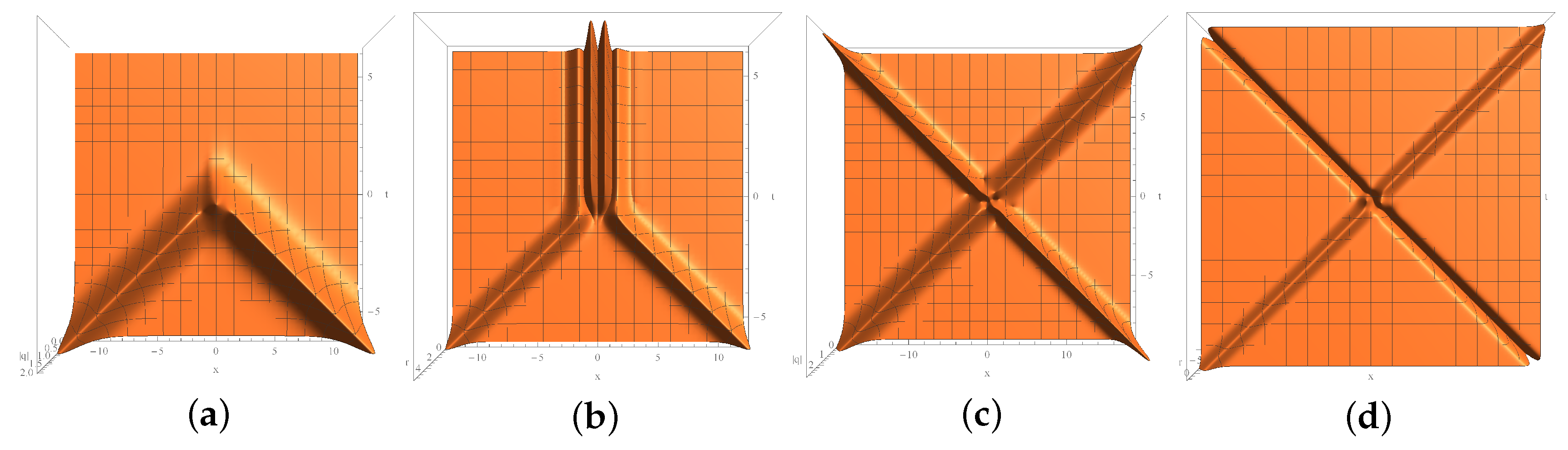
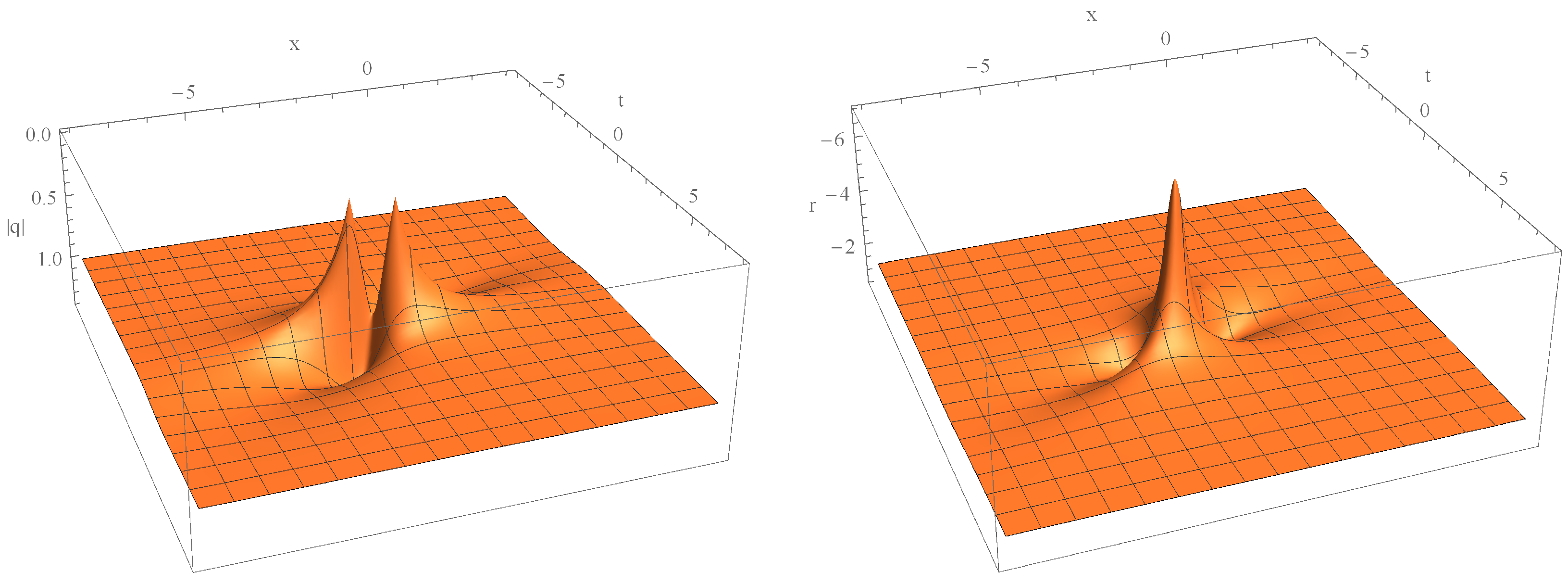
4.2. Case 2. Solutions of Three-Component mYOLS Equation (11)

In the following, we apply the Darboux transformation to give explicit solutions of three-component mYOLS Equation (11). Substituting the trivial solutions $\mathit{q}=0$ and $r=0$ of the three-component mLS Equation (11) into the Riccati Equation (15), we arrive at a system of linear equations

$${\mathit{\rho }}_x=-\lambda \mathit{\varrho },{\mathit{\varrho }}_x=\lambda \mathit{\rho },{\mathit{\rho }}_t=-i{\lambda }^2\mathit{\rho },{\mathit{\varrho }}_t=-i{\lambda }^2\mathit{\varrho },$$

(122)

which possess the general solution:

$$\mathit{\rho }(\lambda )=\mathit{\alpha }(\lambda ){\mathrm{e}}^{ix\lambda -it{\lambda }^2}+\mathit{\beta }(\lambda ){\mathrm{e}}^{-ix\lambda -it{\lambda }^2},\mathit{\varrho }(\lambda )=-i\mathit{\alpha }(\lambda ){\mathrm{e}}^{ix\lambda -it{\lambda }^2}+i\mathit{\beta }(\lambda ){\mathrm{e}}^{-ix\lambda -it{\lambda }^2},$$

(123)

where $\mathit{\alpha }(\lambda )$ and $\mathit{\beta }(\lambda )$ are two constant two-component column vectors of integration.

Solution 1. Assume $N=1$ and choose ${\lambda }_1=1+i$, $\mathit{\alpha }({\lambda }_1)={(1,0)}^T$ and $\mathit{\beta }({\lambda }_1)={(0,1)}^T$. From (123), we deduce an exact solution of the linear Riccati Equation (122)

$$\mathit{\rho }({\lambda }_1)=\left(\begin{array}{c}{\mathrm{e}}^{2t-(1-i)x}\\ {\mathrm{e}}^{2t+(1-i)x}\end{array}\right),\mathit{\varrho }({\lambda }_1)=\left(\begin{array}{c}-i{\mathrm{e}}^{2t-(1-i)x}\\ i{\mathrm{e}}^{2t+(1-i)x}\end{array}\right).$$

(124)

Using the one-fold Darboux transformations (43), (44), and (45), we obtain explicit solutions of the three-component mYOLS Equation (11) (cf.  Figure 7, ${\mathit{q}}_{\underline{a}}={(q_{1,\underline{a}},q_{2,\underline{a}})}^T$),

$$\begin{array}{cc}\hfill & q_{1,\underline{a}}=\frac{(2+2i){\mathrm{e}}^{2t+(1+i)x}(1+2{\mathrm{e}}^{4t+2x})[(1-i){\mathrm{e}}^{4t}-i{\mathrm{e}}^{2x}+4{\mathrm{e}}^{8t+2x}+(1-i){\mathrm{e}}^{4t+4x}]}{{[(1+i){\mathrm{e}}^{4t}+i{\mathrm{e}}^{2x}+4{\mathrm{e}}^{8t+2x}+(1+i){\mathrm{e}}^{4t+4x}]}^2},\hfill \\ \hfill & q_{2,\underline{a}}=\frac{(2+2i){\mathrm{e}}^{2t-(1+i)x}(1+2{\mathrm{e}}^{4t-2x})[(1-i){\mathrm{e}}^{4t}-i{\mathrm{e}}^{2x}+4{\mathrm{e}}^{8t+2x}+(1-i){\mathrm{e}}^{4t+4x}]}{{[(1+i){\mathrm{e}}^{4t}+i{\mathrm{e}}^{2x}+4{\mathrm{e}}^{8t+2x}+(1+i){\mathrm{e}}^{4t+4x}]}^2},\hfill \\ \hfill & r_{\underline{a}}=\frac{8{\mathrm{e}}^{4t+2x}(1-4{\mathrm{e}}^{8t})(1-{\mathrm{e}}^{4x})}{|(1+i){\mathrm{e}}^{4t}+i{\mathrm{e}}^{2x}+4{\mathrm{e}}^{8t+2x}+(1+i){\mathrm{e}}^{4t+4x}{|}^2}.\hfill \end{array}$$

(125)

Solutions 2–5. Similarly, on the basis of (106), (107), and (35), we can obtain explicit solutions of the three-component mYOLS Equation (11) from the two-fold generalized Darboux transformation (90). The results are listed in  

Table 2. Exact solutions for (11) by the two-fold Darboux transformations.

Solution	Figure	${\mathit{\lambda }}_1$	${\mathit{\lambda }}_2$	$\mathit{\alpha }{({\mathit{\lambda }}_1)}^{\mathit{T}}$	$\mathit{\alpha }{({\mathit{\lambda }}_2)}^{\mathit{T}}$	$\mathit{\beta }{({\mathit{\lambda }}_1)}^{\mathit{T}}$	$\mathit{\beta }{({\mathit{\lambda }}_2)}^{\mathit{T}}$
2	Figure 8a–c	$1+i$	$1+2i$	${\mathrm{e}}^{-8}(1,0)$	${\mathrm{e}}^{16+12i}(1,1)$	${\mathrm{e}}^{-8}(1,1)$	${\mathrm{e}}^{16+12i}(0,1)$
3	Figure 8d–f	$1+i$	$1-2i$	${\mathrm{e}}^{-8}(1,0)$	${\mathrm{e}}^{-16+12i}(1,1)$	${\mathrm{e}}^{-8}(1,1)$	${\mathrm{e}}^{-16+12i}(0,1)$
4	Figure 8g–i	$1+i$	$1+2i$	${\mathrm{e}}^8(1,1)$	${\mathrm{e}}^{-16-12i}(1,1)$	${\mathrm{e}}^8(1,0)$	${\mathrm{e}}^{-16-12i}(0,1)$
5	Figure 8j–l	$1+i$	$1-2i$	${\mathrm{e}}^{-8}(1,1)$	${\mathrm{e}}^{-16+12i}(1,1)$	${\mathrm{e}}^{-8}(0,1)$	${\mathrm{e}}^{-16+12i}(1,0)$

.

Remark All the above explicit solutions for the two-component mLS Equation (10) and the three-component mLS Equation (11) have been verified using Mathematica.

5. Conclusions

In the foregoing sections, we derived the Lax pair of a vmYOLS equation. It is difficult to construct a Darboux transformation for the vmYOLS equation because the spectral structure of its Lax pair is too complicated. On the basis of the Riccati equations related to the Lax pair and the gauge transformations between the Lax pairs, a systematic method was developed to construct general N-fold Darboux transformations for the vmYOLS equation. It is worth noting that the general N-fold Darboux transformations of the vmYOLS equation given in Theorem 2 can be reduced to classical N-fold Darboux transformations when ${\mu }_1=\cdots ={\mu }_{\nu }=1$, and can be reduced to generalized N-fold Darboux transformations without taking limits when $\nu =1$. Because we do not have to take the limit when we construct the generalized N-fold Darboux transformations, this simplifies the calculation enormously. Resorting to computer algebra, some exact solutions—including soliton solutions, breather solutions, and rogue-wave solutions—of the vmYOLS equation were obtained using the multi-fold and generalized Darboux transformation.

References

1. Nishikawa, K.; Hojo, H.; Mima, K.; Ikezi, H. Coupled nonlinear electron-plasma and ion-acoustic waves. Phys. Rev. Lett. 1974, 33, 148–151. [Google Scholar] [CrossRef]
2. Kawahara, T.; Sugimoto, N.; Kakutani, T. Nonlinear interaction between short and long capillary-gravity waves. J. Phys. Soc. Jpn. 1975, 39, 1379–1386. [Google Scholar] [CrossRef]
3. Gibbon, J.; Thornhill, S.G.; Wardrop, M.J.; Ter Haar, D. On the theory of Langmuir solitons. J. Plasma Phys. 1977, 17, 153–170. [Google Scholar] [CrossRef]
4. Funakoshi, M.; Oikawa, M. The resonant interactions between a long internal gravity wave and asurface gravity wave packet. J. Phys. Soc. Jpn. 1983, 52, 1982–1995. [Google Scholar] [CrossRef]
5. Yajima, N.; Oikawa, M. Formation and interaction of sonic-Langmuir solitons–inverse scattering method. Progr. Theoret. Phys. 1976, 56, 1719–1739. [Google Scholar] [CrossRef]
6. Ma, Y.C. The complete solution of the long-wave - short-wave resonance equations. Stud. Appl. Math. 1978, 59, 201–221. [Google Scholar] [CrossRef]
7. Zabolotskii, A.A. Inverse scattering transform for the Yajima-Oikawa equations with nonvanishing boundary conditions. Phys. Rev. A 2009, 80, 063616. [Google Scholar] [CrossRef]
8. Leble, S.B.; Ustinov, N.V. Darboux transforms, deep reductions and solitons. J. Phys. A 1993, 26, 5007–5016. [Google Scholar] [CrossRef]
9. Newell, A.C. Long waves-short waves: A solvable model. SIAM J. Appl. Math. 1978, 35, 650–664. [Google Scholar] [CrossRef]
10. Newell, A.C. The general structure of integrable evolution equations. Proc. Roy. Soc. Lond. Ser. A 1979, 365, 283–311. [Google Scholar] [CrossRef]
11. Roy Chowdhury, A.; Chanda, P.K. To the complete integrability of long-wave-short-wave interaction equations. J. Math. Phys. 1986, 27, 707–709. [Google Scholar] [CrossRef]
12. Liu, Q.P. Modifications of k-constrained KP hierarchy. Phys. Lett. A 1994, 187, 373–381. [Google Scholar] [CrossRef]
13. Chowdhury, A.; Tataronis, J.A. Long wave-short wave resonance in nonlinear negative refractive index media. Phys. Rev. Lett. 2008, 100, 153905. [Google Scholar] [CrossRef] [PubMed]
14. Ling, L.M.; Liu, Q.P. A long waves-short waves model: Darboux transformation and soliton solutions. J. Math. Phys. 2011, 52, 053513. [Google Scholar] [CrossRef]
15. Geng, X.G.; Wang, H. Algebro-geometric constructions of quasi-periodic flows of the Newell hierarchy and applications. IMA J. Appl. Math. 2017, 82, 97–130. [Google Scholar] [CrossRef]
16. Albert, J.; Bhattarai, S. Existence and stability of a two-parameter family of solitary waves for an NLS-KdV system. Adv. Diff. Equ. 2013, 18, 1129–1164. [Google Scholar]
17. Guo, B.L.; Miao, C.X. Well-posedness of the Cauchy problem for the coupled system of the Schrödinger-KdV equations. Acta Math. Sin. 1999, 15, 215–224. [Google Scholar] [CrossRef]
18. Albert, J.; Angulo Pava, J. Existence ann stability of ground-state solutions of a Schrödinger-KdV system. Proc. Roy. Soc. Edinburgh Sect. A 2003, 133, 987–1029. [Google Scholar] [CrossRef]
19. Corcho, A.; Linares, F. Well-posedness for the Schrödinger-Korteweg-de Vries system. Trans. Am. Math. Soc. 2007, 359, 4089–4106. [Google Scholar] [CrossRef]
20. Guo, B.L.; Chen, L. Orbital stability of solitary waves of the long wave-short wave resonance equations. Math. Methods Appl. Sci. 1998, 21, 883–894. [Google Scholar] [CrossRef]
21. Chen, J.C.; Feng, B.F.; Maruno, K.I.; Ohta, Y. The derivative Yajima-Oikawa system: Bright, dark soliton and breather solutions. Stud. Appl. Math. 2018, 141, 145–185. [Google Scholar] [CrossRef]
22. Ablowitz, M.J.; Kaup, D.J.; Newell, A.C.; Segur, H. The inverse scattering transform-Fourier analysis for nonlinear problems. Stud. Appl. Math. 1974, 53, 249–315. [Google Scholar] [CrossRef]
23. Ablowitz, M.J.; Segur, H. Solitons and the Inverse Scattering Transform; Society for Industrial and Applied Mathematics (SIAM): Philadelphia, PA, USA, 1981. [Google Scholar]
24. Beals, R.; Coifman, R.R. Inverse scattering and evolution equations. Commun. Pure Appl. Math. 1985, 38, 29–42. [Google Scholar] [CrossRef]
25. Rogers, C.; Schief, W.K. Bäcklund and Darboux Transformations: Geometry and Modern Applications in Soliton Theory; Cambridge University Press: Cambridge, UK, 2010. [Google Scholar]
26. Balakhnev, M.Y.; Demskoi, D.K. Auto-Bäcklund transformations and superposition formulas for solutions of Drinfeld-Sokolov systems. Appl. Math. Comput. 2012, 219, 3625–3637. [Google Scholar] [CrossRef]
27. Matveev, V.B.; Salle, M.A. Darboux Transformations and Solitons; Springer: Berlin/Heidelberg, Germany, 1991. [Google Scholar]
28. Geng, X.G. Lax pair and Darboux transformation solutions of the modified Boussinesq equation. Acta Math. Appl. Sin. 1988, 11, 324–328. [Google Scholar]
29. Geng, X.G. Darboux transformation of the discrete Ablowitz-Ladik eigenvalue problem. Acta Math. Sci. (Engl. Ed.) 1989, 9, 21–26. [Google Scholar] [CrossRef]
30. Geng, X.G.; Tam, H.W. Darboux transformation and soliton solutions for generalized nonlinear Schrödinger equations. J. Phys. Soc. Jpn. 1999, 68, 1508–1512. [Google Scholar] [CrossRef]
31. Geng, X.G.; Lv, Y.Y. Darboux transformation for an integrable generalization of the nonlinear Schrödinger equation. Nonlinear Dynam. 2012, 69, 1621–1630. [Google Scholar] [CrossRef]
32. Lou, S.Y.; Jia, M.; Tang, X.Y.; Huang, F. Vortices, circumfluence, symmetry groups, and Darboux transformations of the (2 + 1)-dimensional Euler equation. Phys. Rev. E 2007, 75, 056318. [Google Scholar] [CrossRef]
33. Shi, Y.; Nimmo, J.J.C.; Zhang, D.J. Darboux and binary Darboux transformations for discrete integrable systems I, Discrete potential KdV equation. J. Phys. A 2014, 47, 025205. [Google Scholar] [CrossRef]
34. Zhou, Z.X. Darboux transformations for the twisted so(p,q) system and local isometric immersion of space forms. Inverse Probl. 1998, 14, 1353–1370. [Google Scholar] [CrossRef]
35. Li, C.X.; Nimmo, J.J.C. Darboux transformations for a twisted derivation and quasideterminant solutions to the super KdV equation. Proc. R. Soc. A 2010, 466, 2471–2493. [Google Scholar] [CrossRef]
36. Chen, J.B.; Pelinovsky, D.E. Rogue periodic waves of the modified KdV equation. Nonlinearity 2018, 31, 1955–1980. [Google Scholar] [CrossRef] [Green Version]
37. Zhang, G.Q.; Yan, Z.Y.; Wen, X.Y. Three-wave resonant interactions: Multi-dark-dark-dark solitons, breathers, rogue waves, and their interactions and dynamics. Physica D 2018, 366, 27–42. [Google Scholar] [CrossRef]
38. Rao, J.G.; Porsezian, K.; He, J.S.; Kanna, T. Dynamics of lumps and dark-dark solitons in the multi-component long-wave-short-wave resonance interaction system. Proc. R. Soc. A 2018, 474, 20170627. [Google Scholar] [CrossRef]
39. Zhao, H.Q.; Yuan, J.Y.; Zhu, Z.N. Integrable semi-discrete Kundu-Eckhaus equation: Darboux transformation, breather, rogue wave and continuous limit theory. J. Nonlinear Sci. 2018, 28, 43–68. [Google Scholar] [CrossRef]
40. Geng, X.G.; Wu, J.P. Riemann-Hilbert approach and N-soliton solutions for a generalized Sasa-Satsuma equation. Wave Motion 2016, 60, 62–72. [Google Scholar] [CrossRef]
41. Xu, J.; Fan, E.G. A Riemann-Hilbert approach to the initial-boundary problem for derivative nonlinear Schrödinger equation. Acta Math. Sci. Ser. B Engl. Ed. 2014, 34, 973–994. [Google Scholar] [CrossRef]
42. Guo, B.L.; Ling, L.M. Riemann-Hilbert approach and N-soliton formula for coupled derivative Schrödinger equation. J. Math. Phys. 2012, 53, 073506. [Google Scholar] [CrossRef]
43. Hirota, R. The Direct Method in Soliton Theory; Cambridge University Press: Cambridge, UK, 2004. [Google Scholar]
44. Geng, X.G.; Li, R.M.; Xue, B. A new integrable equation with peakons and cuspons and its bi-Hamiltonian structure. Appl. Math. Lett. 2015, 46, 64–69. [Google Scholar] [CrossRef]
45. Lenells, J. Traveling wave solutions of the Camassa-Holm equation. J. Diff. Equ. 2005, 217, 393–430. [Google Scholar] [CrossRef]
46. Geng, X.G.; Li, R.M. Darboux transformation of the Drinfeld-Sokolov-Satsuma-Hirota system and exact solutions. Ann. Phys. 2015, 361, 215–225. [Google Scholar] [CrossRef]
47. Wazwaz, A.M. The Cole-Hopf transformation and multiple soliton solutions for the integrable sixth-order Drinfeld-Sokolov-Satsuma-Hirota equation. Appl. Math. Comput. 2009, 207, 248–255. [Google Scholar] [CrossRef]
48. Wazwaz, A.M. Exact and explicit travelling wave solutions for the nonlinear Drinfeld-Sokolov system. Commun. Nonlinear Sci. Numer. Simul. 2006, 11, 311–325. [Google Scholar] [CrossRef]
49. Yan, Z.Y. Abundant new explicit exact soliton-like solutions and Painlevé test for the generalized Burgers equation in (2+1)-dimensional space. Commun. Theor. Phys. (Beijing) 2001, 36, 135–138. [Google Scholar]
50. Geng, X.G.; Liu, H. The nonlinear steepest descent method to long-time asymptotics of the coupled nonlinear Schrödinger equation. J. Nonlinear Sci. 2018, 28, 739–763. [Google Scholar] [CrossRef]
51. Ma, W.X.; Zhou, Y. Lump solutions to nonlinear partial differential equations via Hirota bilinear forms. J. Diff. Equ. 2018, 264, 2633–2659. [Google Scholar] [CrossRef]
52. Osborne, A.R. Nonlinear Ocean Waves and the Inverse Scattering Transform; Elsevier/Academic Press: Boston, MA, USA, 2010. [Google Scholar]
53. Ruban, V.; Kodama, Y.; Ruderman, M.; Dudley, J.; Grimshaw, R.; McClintock, P.V.E.; Onorato, M.; Kharif, C.; Pelinovsky, E.; Soomere, T.; et al. Rogue waves–towards a unifying concept?: Discussions and debates. Eur. Phys. J. Special Top. 2010, 185, 5–15. [Google Scholar] [CrossRef]
54. Bludov, V.Y.; Konotop, V.V.; Akhmediev, N. Matter rogue waves. Phys. Rev. A 2009, 80, 033610. [Google Scholar] [CrossRef] [Green Version]
55. Solli, D.R.; Ropers, C.; Koonath, P.; Jalali, B. Optical rogue waves. Nature 2007, 450, 1054–1057. [Google Scholar] [CrossRef]
56. Shats, M.; Punzmann, H.; Xia, H. Capillary rogue waves. Phys. Rev. Lett. 2010, 104, 104503. [Google Scholar] [CrossRef] [PubMed]
57. Onorato, M.; Residori, S.; Baronio, F. (Eds.) Rogue and Shock Waves in Nonlinear Dispersive Media; Springer: Basel, Switzerland, 2016. [Google Scholar]
58. Wang, X.; Liu, C.; Wang, L. Rogue waves and W-shaped solitons in the multiple self-induced transparency system. Chaos 2017, 27, 093106. [Google Scholar] [CrossRef] [PubMed] [Green Version]
59. Rao, J.G.; Wang, L.H.; Liu, W.; He, J.S. Rogue-wave solutions of the Zakharov equation. Theoret. Math. Phys. 2017, 193, 434–454. [Google Scholar] [CrossRef]
60. Chan, H.N.; Malomed, B.A.; Chow, K.W.; Ding, E. Rogue waves for a system of coupled derivative nonlinear Schrödinger equations. Phys. Rev. E. 2016, 93, 012217. [Google Scholar] [CrossRef] [PubMed]
61. Wang, X.; Liu, C.; Wang, L. Darboux transformation and rogue wave solutions for the variable-coefficients coupled Hirota equations. J. Math. Anal. Appl. 2017, 449, 1534–1552. [Google Scholar] [CrossRef]
62. Wei, J.; Wang, X.; Geng, X.G. Periodic and rational solutions of the reduced Maxwell-Bloch equations. Commun. Nonlinear Sci. Numer. Simul. 2018, 59, 1–14. [Google Scholar] [CrossRef]
Figure 1. A one-soliton solution given by a one-fold Darboux transformation.
Mathematics 07 00958 g001
Figure 2. Inelastic (a,b) and elastic (c,d) collisions.
Mathematics 07 00958 g002
Figure 3. Density plot of (c,d) in Figure 2, with the auxiliary lines x = ± 2 t .
Mathematics 07 00958 g003
Figure 4. Some nonlinear interactions.
Mathematics 07 00958 g004
Figure 5. Solution obtained from generalized Darboux transformation.
Mathematics 07 00958 g005
Figure 6. A rogue-wave solution.
Mathematics 07 00958 g006
Figure 7. A soliton given by one-fold Darboux transformation.
Mathematics 07 00958 g007
Figure 8. Some nonlinear interactions.
Mathematics 07 00958 g008