Non-Stationary Acceleration Strategies for PageRank Computing

Abstract

In this work, a non-stationary technique based on the Power method for accelerating the parallel computation of the PageRank vector is proposed and its theoretical convergence analyzed. This iterative non-stationary model, which uses the eigenvector formulation of the PageRank problem, reduces the needed computations for obtaining the PageRank vector by eliminating synchronization points among processes, in such a way that, at each iteration of the Power method, the block of iterate vector assigned to each process can be locally updated more than once, before performing a global synchronization. The parallel implementation of several strategies combining this novel non-stationary approach and the extrapolation methods has been developed using hybrid MPI/OpenMP programming. The experiments have been carried out on a cluster made up of 12 nodes, each one equipped with two Intel Xeon hexacore processors. The behaviour of the proposed parallel algorithms has been studied with realistic datasets, highlighting their performance compared with other parallel techniques for solving the PageRank problem. Concretely, the experimental results show a time reduction of up to $58.4\%$ in relation to the parallel Power method, when a small number of local updates is performed before each global synchronization, outperforming both the two-stage algorithms and the extrapolation algorithms, more sharply as the number of processes increases.

1. Introduction

The PageRank algorithm is a well-known algorithm used for determining the relevance of Web pages [1]. From a theoretical point of view, for solving this problem, we need to obtain the stationary distribution of a discrete-time, finite-state Markov chain, whose transition probability matrix P is obtained as follows—given an ordered set of n Web pages, let us consider the associated adjacency matrix $G={[g_{ij}]}_{i,j=1}^n$, where $g_{ij}=1$ when there is a link from page j to page i, with $i\ne j$, and $g_{ij}=0$ otherwise. This adjacent matrix leads us to the transition matrix $P={[p_{ij}]}_{i,j=1}^n$ defined in the following manner:

$$p_{ij}=\left\{\begin{array}{cc}\frac{g_{ij}}{c_j},\hfill & \mathrm{if}{c}_j=\sum _{i=1}^n{g}_{ij}\ne 0,\hfill \\ 0,\hfill & \mathrm{otherwise}.\hfill \end{array}\right.$$

Note that $c_j$ represents the number of out-links from a page j. In this way, the PageRank vector is a probability vector x such that $Px=x$, with ${\parallel x\parallel }_1={\sum }_{i=1}^n|x_i|={\sum }_{i=1}^n{x}_i=1$.

Definition 1

([2]). A matrix $P=[p_{ij}]\in {\Re }^{n\times n}$ is a column stochastic matrix if it satisfies the following conditions:

(i) 

$p_{ij}\ge 0,\forall i,j=1,2,\dots ,n.$

(ii) 

${\sum }_{i=1}^n{p}_{ij}=1,\forall j=1,2,\dots ,n.$

When the transition matrix P is column stochastic and irreducible (i.e., its graph is strongly connected) there exists a unique positive PageRank vector and we can use the Power method [3] to obtain it. Algorithm 1 explains the original Power method for computing the PageRank vector, where $e={(1,1,\dots ,1)}^T$.

Algorithm 1: Power method.

However, the Web contains dangling pages—that is, pages without out-links—and in this case the matrix P is non-stochastic. Moreover, the Web graph is usually not irreducible. Therefore, the convergence of Algorithm 1 is not ensured. In order to get over these problems, Page and Brin [1] replace the transition matrix P with a column stochastic matrix $\overline{P}=\alpha (P+v{d}^T)+(1-\alpha )v{e}^T$, where $d\in {\Re }^n$ is defined by $d_i=1$ if and only if page i has not any out-link (i.e., $c_i=0$), and the vector $v\in {\Re }^n$ is some probability distribution over pages. Originally $v=\frac{e}{n}$ was used. The parameter $\alpha$ is called the damping factor and determines the weight given to the actual Web link graph in the model. Setting $\alpha$ such that $0<\alpha <1$, the matrix $\overline{P}$ is column stochastic, irreducible and it satisfies that $\parallel \overline{P}{x\parallel }_1={\parallel x\parallel }_1$, that is, $\overline{P}$ preserves the $L_1$ norm. Hence, Algorithm 1 can be reformulated using the matrix $\overline{P}$ for computing the PageRank vector; see Algorithm 2.

Algorithm 2: Power method for solving $\overline{P}x=x$.

Although Algorithm 2 was initially used for ranking Web pages, setting as damping factor $\alpha =0.85$ [1], this algorithm has become very useful in other scientific and technical application areas such as Computational Molecular Biology, Bioinformatics [4,5] and Geographical Information Science [6], where $\alpha$ often has a concrete meaning and the graph structure may not resemble the structure of the Web link graph. Moreover, the study of the behaviour of the PageRank vectors with respect to changes in $\alpha$ is being used for detecting link spammers [7,8]. In addition, a PageRank model is more realistic as the parameter $\alpha$ is closer to 1. However, as $\alpha$ increases, the number of iterations required for convergence of Algorithm 2 grows dramatically [2]. Therefore, new techniques for accelerating its computations are needed. Over the last years, different strategies to accelerate the Power method have been analyzed, such as extrapolation methods [9], adaptive methods [10] and Arnoldi-type algorithms [11,12,13]. These listed acceleration methods are based on the eigenvector formulation of the PageRank problem. Recently, some approaches based on the linear system formulation of the PageRank problem have also been studied [14,15,16,17].

The Arnoldi-type algorithm proposed in Reference [11] is a restarted Krylov subspace method, obtained by combining the Arnoldi process and small singular value decomposition that relies on the knowledge of the largest eigenvalue. The experiments performed in Reference [11] compare the rate of convergence by means of the number of iterations needed for convergence of the designed Arnoldi-type algorithm with respect to the Power method, obtaining that this method does not improve the Power method, when the damping factor $\alpha$ is small (e.g., $\alpha =0.85$). Similar conclusions were reached about the efficiency of the Power method for small values of $\alpha$ compared with the quadratic extrapolation method [9] and with approaches based on the linear system formulation of the PageRank problem [14].

Although no numerical experiments about the running time needed for the convergence of this Arnoldi-type algorithm were done in Reference [11], as it was shown in a more recent work [13], the Arnoldi-type algorithms may not be efficient when the damping factor $\alpha$ is high and the dimension of the search subspace is small. The code for the experiments performed in Reference [13] was implemented in Matlab and executed in a sequential mode.

However, taking into account the large size of the Web link graph, parallel processing becomes necessary for computing the PageRank vector. In Reference [14], parallel algorithms based on Krylov subspace methods are analyzed, showing that although these methods reduce the number of iterations needed for computing PageRank, on some graphs, their parallel implementation does not provide time saving in relation to the parallel Power method. In Reference [15], a parallel inner-outer algorithm is proposed for the dense linear system formulation of the PageRank problem, achieving a substantial gain with respect to the Power method, specially when $\alpha$ is close to 1. In Reference [18], parallel algorithms based on the Power extrapolation methods are considered, showing that these algorithms can outperform the inner-outer Power algorithm proposed in Reference [15]. However, their convergence speed depends on a good choice of the different parameters involved in these methods. In order to overcome this limitation, a heuristic based on the parallel algorithms designed in Reference [18] was constructed in Reference [19]. In Reference [20], new parallel algorithms for computing PageRank are designed based on the sparse linear system formulation of the PageRank problem. The displayed numerical experiments showed that these algorithms, based on the two-stage methods [21], can achieve better results than both the extrapolation Power methods [18] and the inner-outer techniques proposed in Reference [15]; other related works can be found, for example, in References [22,23,24,25].

In this paper, using the eigenvector formulation of the problem, a non-stationary technique based on the Power method for accelerating the parallel computation of PageRank is proposed. These non-stationary methods aim to reduce the number of global iterations of the Power method, by eliminating synchronization points at which a process must wait for information from the remaining processes. In Section 2 we describe this iterative technique and we show its convergence. Section 3 reports the parallel implementation details and the different strategies considered for computing PageRank. Section 4 displays experimental results showing the behaviour of the designed algorithms for realistic test data on a current Symmetric Multi-Processing (SMP) supercomputer. Finally, some conclusions are presented in Section 5.

2. Non-Stationary Power Algorithms: Design and Convergence Analysis

Let us consider $P={\left[P_1^t{P}_2^t\cdots P_p^t\right]}^t$, where each row block $P_i$, $1\le i\le p$, is a matrix of order $n_i\times n$, with ${\sum }_{i=1}^p{n}_i=n$. Analogously, we consider the iterate vectors $x^{(l)}$ and v partitioned according to the block structure of P. Obviously, the Power method for solving $\overline{P}x=x$ (Algorithm 2) can be executed in parallel. In this case, each process actualizes one of the p blocks of the vector $x^{(l+1)}$ and a synchronization of all processes is needed, at the end of each iteration, to construct the global iterate vector $x^{(l+1)}$. Due to this synchronization, the property of preserving the $L_1$ norm remains valid and therefore the formulation of Algorithm 2 can be used for designing this parallel version of the Power method.

Taking into account that the Power iterations on web-sized matrices are so expensive, different strategies for accelerating the computation of PageRank can be considered. First of all, in order to reduce the synchronizations between processes we can consider a non-stationary strategy in which the block of the vector $x^{(l+1)}$ assigned to a process is updated more than once before all processes synchronize on a barrier, that is to say, each process i actualizes $q(i)$ times the iterate vector $x_i^{(l+1)}$ before a synchronization is done. However, the condition of preserving the $L_1$ norm is not ensured in this last case. Therefore, Algorithm 2 can not be used for our purpose in its current formulation. For this reason, we have proposed an equivalent formulation of Algorithm 2 in which the condition on the $L_1$ norm is not needed. That is, if Algorithm 1 is applied on the matrix $\overline{P}$, some algebraic manipulations yields:

$$\begin{array}{ccc}\hfill x^{(l+1)}& =& \overline{P}{x}^{(l)}\hfill \\ & =& \alpha (P+v{d}^T)x^{(l)}+(1-\alpha )v{e}^T{x}^{(l)}\hfill \\ & =& \alpha P{x}^{(l)}+\alpha v{d}^T{x}^{(l)}+(1-\alpha )v{e}^T{x}^{(l)}\hfill \\ & =& \alpha P{x}^{(l)}+\alpha d^T{x}^{(l)}v+(1-\alpha ){\parallel x^{(l)}\parallel }_{1}v.\hfill \end{array}$$

(1)

Taking into account (1), Algorithm 3 shows the above mentioned non-stationary strategy. Note that although the matrix $\overline{P}$ is dense, it is not necessary to explicitly construct it.

Algorithm 3: Parallel non-stationary algorithm for solving PageRank.

Alternatively, the synchronizations between processes can be eliminated in the sense that each process updates parts of the current iterate without waiting for the other parts of $x^{(l)}$ to be updated. Instead, processes use a vector composed of parts of different previous, not necessarily the latest, iterates; see, for example, Reference [26].

In order to describe this asynchronous version let us define the sets $J_l\subseteq \{1,2,\dots ,p\},l=1,2,\dots$, by $i\in J_l$ if the ith block of the vector $x^{(l)}$ is computed at the lth iteration. The values $r(l,i)$ are used to denote the iteration number of the ith block being used in the computation of any block at the lth iteration. Let us denote by $H_i(x)=y_i$ the operator that performs the following computations:

$$\begin{array}{ccc}\hfill y_i& =& \alpha P_{i}x\hfill \\ \hfill \gamma & =& \alpha d^{T}x+(1-\alpha ){\parallel x\parallel }_1\hfill \\ \hfill y_i& =& y_i+\gamma v_i.\hfill \end{array}$$

With this notation, Algorithm 4 describes the asynchronous Power method for solving PageRank.

Algorithm 4: Parallel asynchronous Power method for solving PageRank.

Note that the local convergence of the processes in an asynchronous iterative algorithm does not ensure its global convergence. In order to ensure the convergence of Algorithm 4 we assume that the asynchronous iterations satisfy the following common conditions; see, for example, Reference [27].

$$\begin{array}{c}r(l,i)<l,\forall l=1,2,\dots ,1\le i\le p.\hfill \end{array}$$

(2)

$$\begin{array}{c}\underset{l\to \infty }{lim}r(l,i)=\infty ,1\le i\le p.\hfill \end{array}$$

(3)

$$\begin{array}{c}\text{The set}\{l|i\in J_l\}\text{is unbounded for all}1\le i\le p.\hfill \end{array}$$

(4)

Assumption (2) implies that only previously computed iterate vectors can be used, while condition (3) ensures that iterates computed too far away are not used; condition (4) states that all vector blocks are always computed as the iteration proceed. Under conditions (2)–(4), taking into account that the problem involves a nonnegative stochastic and irreducible matrix with a spectral radius equal to 1, from Reference [28] it follows that Algorithm 4 converges to the PageRank vector corresponding to the analyzed Web pages, performing a simple normalization at the end of the algorithm.

While Algorithm 3 can be implemented on shared, distributed and distributed shared architectures, the implementation of an asynchronous algorithm like the one described in Algorithm 4 presents many difficulties on both distributed and distributed shared memory architectures since nodes have only local information, there is no global clock, and the delays may be unpredictable. Moreover, the results obtained in a previous work about the parallelization of the PageRank problem [25] showed that the synchronous and asynchronous execution times of the Power method are, in general, very similar on a shared memory computer; depending on the graph and on the number of cores used, one algorithm is better than the other. The reason resides presumably in a different density pattern of the matrices. In a matrix in which the density pattern is not homogeneous along the files assigned to each process, an asynchronous execution will avoid processes to be inactive, waiting for other processes to finish their computations. In fact, as it was studied in Reference [25], in the asynchronous case, each process performs a different number of iterations, but the minimum over all processes is close to the number of iterations of the corresponding synchronous execution. In the best case, all processes perform similar iterations while in other cases there are processes that perform more than twice iterations.

Taking all this into consideration, Algorithm 3 can be an alternative for the parallel computation of the PageRank vector in order to eliminate some limitations in practice of Algorithm 4.

From a theoretical point of view, it is possible to show that the parallel non-stationary method for solving PageRank described in Algorithm 3 can be seen as a particular case of the parallel asynchronous method defined by Algorithm 4 satisfying conditions (2)–(4), and therefore convergence of Algorithm 3 would also be ensured. For this purpose, we need to make a definition for all the parameters involved in the description of the asynchronous Algorithm 4, in such a way that this asynchronous algorithm leads to the same iterate vectors computed by Algorithm 3. First, let us define $s(i),i=1,2,\dots ,p$, as follows:

$$\begin{array}{ccc}\hfill s(1)& =& q(1),\hfill \\ \hfill s(i)& =& s(i-1)+q(i),i=2,3,\dots ,p.\hfill \end{array}$$

Also, let us denote by T the sum of all values $q(i),i=1,2,\dots ,p$, that is, $T={\sum }_{i=1}^{p}q(i)=s(p)$. On the other hand, let us define the sets $J_l$, for all $l\ge 1$, according to Algorithm 5, where $a\backslash b$ denotes the integer division between two integers $a,b$.

Algorithm 5:$J_l$ set definition, $l\ge 1$.

By analyzing Algorithm 5, it is observed that, at the first T iterations, the sets $I_i$, defined as

$$\begin{array}{ccc}\hfill I_1& =& \left\{a\in {\mathbb{Z}}^{+}|a\in \left[init(1),end(1)\right]\right\}=\left\{a\in {\mathbb{Z}}^{+}|a\in \left[1,q(1)\right]\right\},\hfill \\ \hfill I_i& =& \left\{a\in {\mathbb{Z}}^{+}|a\in \left[init(i),end(i)\right]\right\}\hfill \\ & =& \left\{a\in {\mathbb{Z}}^{+}|a\in \left[q(1)+q(2)+\dots +q(i-1)+1,q(1)+q(2)+\dots +q(i)\right]\right\},i=2,3,\dots ,p,\hfill \end{array}$$

are a partition of the set $\{1,2,\dots ,T\}$, that is, $I_i\ne \varnothing ,{\bigcup }_{i=1}^p{I}_i=\{1,2,\dots ,T\}$ and $I_i\cap I_j=\varnothing ,i\ne j$. Therefore, every element l of the set $\{1,2,\dots ,T\}$ will belong to a unique set $I_i$, that is, line 7 of Algorithm 5 is well defined. Similarly, we conclude that the above is true for the next T iterations and so on.

To finish with the description of the asynchronous parameters, let us define the values $r(l,i),l=1,2,\dots ,1\le i\le p$ as in Algorithm 6.

Algorithm 6: Asynchronous parameters $r(l,i),l=1,2,\dots ,1\le i\le p$.

Therefore, for showing the convergence of Algorithm 3, first we need to show that the parameters $r(l,i)$ defined in Algorithm 6 and the sets $J_l$ defined in Algorithm 5 verify conditions (2)–(4).

Proposition 1.

Let us consider the parameters $r(l,i),l=1,2,\dots ,1\le i\le p$, defined in Algorithm 6 and the sets $J_l,l=1,2,\dots$, defined in Algorithm 5. Then, the parameters $r(l,i)$ and the sets $J_l$ satisfy conditions (2)–(4).

Proof. 

From line 6 of Algorithm 6, it follows

$$\begin{array}{ccc}\hfill 0\le tmp& \le & T((l-1)\backslash T)\le T\frac{l-1}{T}=l-1<l, \mathrm{and}\hfill \\ \hfill tmp& >& T((l-1)\backslash T)-T>T(\frac{l-1}{T}-1)-T=(l-1)-2T.\hfill \end{array}$$

Therefore, from lines 8 and 11 of Algorithm 6 it follows that conditions (2) and (3) are true. On the other hand, from the definition of the sets $J_l$ in Algorithm 5 it follows that for all $1\le i\le p$, $J_l=\{i\}$ at least once in every T consecutive asynchronous iterations, concretely $q(i)$ times (see, e.g.,

Table 1. Example of equivalence between non-stationary synchronous and asynchronous iterations, $p=4$ and $(q(1),q(2),q(3),q(4))=(2,3,1,2)$.

Asynchronous Iterations (See Algorithm 4)							Synchronous Iterations (Algorithm 3)
Iter. l	$r(l,1)$	$r(l,2)$	$r(l,3)$	$r(l,4)$	computed block: $J_l$	$x^{(l)}$	Iter.	$x^{(l)}$
1	0	0	0	0	$\{1\}$	$x_1^{(1)}=H_1(x_1^{(0)},x_2^{(0)},x_3^{(0)},x_4^{(0)})$	1	$y_1^{(q(1))}$
2	1	0	0	0	$\{1\}$	$x_1^{(2)}=H_1(x_1^{(1)},x_2^{(0)},x_3^{(0)},x_4^{(0)})$
3	0	0	0	0	$\{2\}$	$x_2^{(3)}=H_2(x_1^{(0)},x_2^{(0)},x_3^{(0)},x_4^{(0)})$		$y_2^{(q(2))}$
4	0	3	0	0	$\{2\}$	$x_2^{(4)}=H_2(x_1^{(0)},x_2^{(3)},x_3^{(0)},x_4^{(0)})$
5	0	4	0	0	$\{2\}$	$x_2^{(5)}=H_2(x_1^{(0)},x_2^{(4)},x_3^{(0)},x_4^{(0)})$
6	0	0	0	0	$\{3\}$	$x_3^{(6)}=H_3(x_1^{(0)},x_2^{(0)},x_3^{(0)},x_4^{(0)})$		$y_3^{(q(3))}$
7	0	0	0	0	$\{4\}$	$x_4^{(7)}=H_4(x_1^{(0)},x_2^{(0)},x_3^{(0)},x_4^{(0)})$		$y_4^{(q(4))}$
8	0	0	0	7	$\{4\}$	$x_4^{(8)}=H_4(x_1^{(0)},x_2^{(0)},x_3^{(0)},x_4^{(7)})$
The above first 8 asynchronous iterations are equivalent to the synchronous iteration 1: $(x_1^{(2)},x_2^{(5)},x_3^{(6)},x_4^{(8)})=(y_1^{(q(1))},y_2^{(q(2))},y_3^{(q(3))},y_4^{(q(4))})$ This vector is used in the next asynchronous and synchronous iterations.
9	2	5	6	8	$\{1\}$	$x_1^{(9)}=H_1(x_1^{(2)},x_2^{(5)},x_3^{(6)},x_4^{(8)})$	2	$y_1^{(q(1))}$
10	9	5	6	8	$\{1\}$	$x_1^{(10)}=H_1(x_1^{(9)},x_2^{(5)},x_3^{(6)},x_4^{(8)})$
11	2	5	6	8	$\{2\}$	$x_2^{(11)}=H_2(x_1^{(2)},x_2^{(5)},x_3^{(6)},x_4^{(8)})$		$y_2^{(q(2))}$
12	2	11	6	8	$\{2\}$	$x_2^{(12)}=H_2(x_1^{(2)},x_2^{(11)},x_3^{(6)},x_4^{(8)})$
13	2	12	6	8	$\{2\}$	$x_2^{(13)}=H_2(x_1^{(2)},x_2^{(12)},x_3^{(6)},x_4^{(8)})$
14	2	5	6	8	$\{3\}$	$x_3^{(14)}=H_3(x_1^{(2)},x_2^{(5)},x_3^{(6)},x_4^{(8)})$		$y_3^{(q(3))}$
15	2	5	6	8	$\{4\}$	$x_4^{(15)}=H_4(x_1^{(2)},x_2^{(5)},x_3^{(6)},x_4^{(8)})$		$y_4^{(q(4))}$
16	2	5	6	15	$\{4\}$	$x_4^{(16)}=H_4(x_1^{(2)},x_2^{(5)},x_3^{(6)},x_4^{(15)})$
The above 8 asynchronous iterations are equivalent to the synchronous iteration 2: $(x_1^{(10)},x_2^{(13)},x_3^{(14)},x_4^{(16)})=(y_1^{(q(1))},y_2^{(q(2))},y_3^{(q(3))},y_4^{(q(4))})$ This vector is used in the next asynchronous and synchronous iterations.
17	10	13	14	16	$\{1\}$	$x_1^{(17)}=H_1(x_1^{(10)},x_2^{(13)},x_3^{(14)},x_4^{(16)})$	3	$y_1^{(q(1))}$
18	17	13	14	16	$\{1\}$	$x_1^{(18)}=H_1(x_1^{(17)},x_2^{(13)},x_3^{(14)},x_4^{(16)})$
19	10	13	14	16	$\{2\}$	$x_2^{(19)}=H_2(x_1^{(10)},x_2^{(13)},x_3^{(14)},x_4^{(16)})$		$y_2^{(q(2))}$
20	10	19	14	16	$\{2\}$	$x_2^{(20)}=H_2(x_1^{(10)},x_2^{(19)},x_3^{(14)},x_4^{(16)})$
21	10	20	14	16	$\{2\}$	$x_2^{(21)}=H_2(x_1^{(10)},x_2^{(20)},x_3^{(14)},x_4^{(16)})$
22	10	13	14	16	$\{3\}$	$x_3^{(22)}=H_3(x_1^{(10)},x_2^{(13)},x_3^{(14)},x_4^{(16)})$		$y_3^{(q(3))}$
23	10	13	14	16	$\{4\}$	$x_4^{(23)}=H_4(x_1^{(10)},x_2^{(13)},x_3^{(14)},x_4^{(16)})$		$y_4^{(q(4))}$
24	10	13	14	23	$\{4\}$	$x_4^{(24)}=H_4(x_1^{(10)},x_2^{(13)},x_3^{(14)},x_4^{(23)})$
The above 8 asynchronous iterations are equivalent to the synchronous iteration 3: $(x_1^{(18)},x_2^{(21)},x_3^{(22)},x_4^{(24)})=(y_1^{(q(1))},y_2^{(q(2))},y_3^{(q(3))},y_4^{(q(4))})$ This vector is used in the next asynchronous and synchronous iterations.
⋮	⋮	⋮	⋮	⋮	⋮	⋮	⋮	⋮

for an illustrative example). Therefore, the set $\{l|i\in J_l\}$ is clearly unbounded for all $1\le i\le p$ and therefore assumption (4) is satisfied. □

Now, we are in a position to prove the convergence of the parallel non-stationary Algorithm 3.

Theorem 1.

Let P be the transition matrix of the PageRank problem. Then, the parallel non-stationary Algorithm 3 converges to the PageRank vector performing a simple normalization at the end of the algorithm.

Proof. 

Taking into account Equation (1) and Proposition 1, to show the convergence of Algorithm 3 we need to show that the sequence of iterate vectors generated by Algorithm 4 with the asynchronous parameters defined in Algorithms 5 and 6, corresponds to the sequence generated by Algorithm 3. For this purpose, first note that the cardinality of the sets $J_l$ indicates that only one block of the iterate vector (of the p blocks) is updated at each asynchronous iteration. On the other hand, note that a set of T consecutive asynchronous iterations is equivalent to one iteration of Algorithm 3. Also, note that, after these T asynchronous iterations are completed, a new iteration starts with the most recent values obtained in previous iterations, which is equivalent to a synchronization in Algorithm 3. In order to more clearly visualize this equivalence we show in Table 1 an example of how the asynchronous iterations match the synchronous counterpart. Therefore, as the matrix $\overline{P}$ is a non-negative stochastic and irreducible matrix with spectral radius equal to 1, from [28] the convergence of Algorithm 4 and hence the convergence of Algorithm 3 is ensured. □

3. Parallel Implementation

Taking into account the study carried out in Section 2, we propose and analyze different strategies based on the non-stationary technique. These strategies are summarized in Algorithm 7.

Algorithm 7: Parallel algorithms for solving PageRank.

The first algorithm, which we have called MSTEP algorithm, corresponds to Algorithm 7 setting $ext\ne 1$, that is, in the MSTEP algorithm, lines from 3 to 14 are not executed, yielding to a parallel non-stationary Power algorithm (lines from 15 to 30) in which each part of $x^{(l+1)}$ ($x_i^{(l+1)}$) can be updated more than once ($q(i)\ge 1$ times) without waiting for the other parts of $x^{(l+1)}$ to be updated and therefore eliminating synchronization points among processes. When $ext=1$, Algorithm 7 explains a second algorithm, called the EMS algorithm. The first part of this algorithm (first repeat-until loop) consists in applying $r+2$ Power iterations, that is, each part of $x^{(l+1)}$ is updated only once at each lth iteration, performing an extrapolation at the last $r+2$ iteration (see line 8). This extrapolation is applied only once. Note that if $r=1$, a simple extrapolation is performed at iteration 3, while if $r=2$ a quadratic extrapolation is applied once at iteration 4. In the second part of the EMS algorithm (second repeat-until loop), after the extrapolation has been performed, each part of $x^{(l+1)}$ is again updated but more than once without synchronizing with the remaining processes. This strategy can be seen as a particular case of a non-stationary algorithm in which an initial vector nearest to the solution is used as initial vector.

On the other hand, a relaxation parameter $\beta >0$ can be introduced in the EMS algorithm and replace the computation of $x_i^{(l+1)}$ in line 23 with the equation $x_i^{(l+1)}=\beta y_i^{(q(i))}+(1-\beta )x_i^{(l)}$, obtaining its relaxed counterpart which we have called the RELEMS algorithm. Note that, at each global iteration of the second repeat-until loop, each process computes the relaxation of its vector block before the synchronization among processes has been accomplished. Clearly, with $\beta =1$ the EMS algorithm is recovered.

The algorithms described here have been implemented in C++ on an HPC cluster of 12 nodes HP Proliant SL390s G7 connected through a network of low-latency QDR Infiniband-based. Each node consists of two Intel XEON X5660 hexacore at up to 2.8 GHz and 12 MB cache per processor, with 48 GB of RAM. The operating system is CentOS Linux 5.6 for ×86 64 bit.

Taking into account the hierarchical hardware design of this HPC cluster, the parallel programming of these algorithms has been done combining distributed memory parallelization on the node interconnect with shared memory parallelization inside each node. For this purpose, there is the option to use pure MPI (Message Passing Interface) [29] and treat every CPU core as a separate entity with its own address space. However, in this work we have combined the MPI and OpenMP (Open Multi-Processing) [30] programming models into a hybrid paradigm, exploiting parallelism beyond a single level. Adding OpenMP threading to an MPI code can be an efficient way to run on multicore processors that are part of a multinode system like this HPC cluster. Since OpenMP operates in a shared memory space, it is possible to reduce the memory overhead associated with MPI tasks and reduce the need for replicated data across tasks [19]. In this way, the parallel environment has been managed using a hybrid MPI/OpenMP model. In order to explain and analyze this hybrid model, we have used similar notation to that used in our previous works [18,19,20]. Concretely, $s\times c$ means that s nodes of the HPC cluster are utilized for data distribution and for each one of these nodes, c OpenMP threads are considered. That is, we consider a distributed shared memory (DSM) model with $p=s\times c$ processes or threads. With this notation, if $c=1$ the algorithms are executed in distributed memory (DM) using s nodes, while if $s=1$ the execution of the algorithms is performed using c threads on a single node, that is, in shared memory (SM).

For the sake of clarity, we can consider that Algorithm 7 describes the parallelization of the non-stationary methods using a distributed memory programming in such a way that each one of the p MPI processes is assigned to a physical node. Then, in the distributed shared memory implementation, a number of OpenMP threads are spawned by every MPI process in order to execute in parallel the computation of lines 5–8, 10, 18–20, 25 and 27. The loop that implements every of these computations is headed with a “parallel for” pragma (“#pragma omp parallel for”). This parallel OpenMP pragma spawns a group of threads and splits the loop iterations between the spawned threads following some system-specific strategy. On the other hand, a dynamic scheduling scheme was used for partitioning the work related to lines 5 and 18. In this dynamic strategy, groups of size determined by the user are allocated to the threads following a first-come, first-served scheme. According to the nonzero pattern of the matrix P, a static scheme for distributing the work could cause a different number of nonzero elements of the matrix P allocated from one thread to another, leading to an unbalanced computational cost of the work associated with lines 5 and 18. Therefore, this dynamic scheduling scheme was preferable over a static strategy. The computation of lines 6, 10, 19, 25 and 27 needs a reduction operation when the OpenMP parallel region ends. In this computation, as well as in the rest of the parallel tasks, a static scheduling scheme ensures, a priori, a load balancing among threads. However, if this static strategy is used, the number of fork/join concurrency control mechanisms is incremented. In order to avoid this increase of fork/join operations, we have included these computations in the previous dynamic OpenMP “parallel for,” namely line 5 or 18.

4. Numerical Experiments and Results

In order to investigate and analyze the algorithms described here, we have used several datasets of different sizes, available from the Laboratory for Web Algorithmics [31]; see

Table 2. Graphs collection. n = number of nodes, nnz =number of arcs, Dgn = percentage of dangling nodes, Dens = density (arcs/nodes), M = memory requirements using $mCSR$ format.

Graph	n	nnz	Dgn (%)	Dens	M (GB)
uk-2002	18,520,486	298,113,762	14.91	16.01	1.32
it-2004	41,291,594	1,150,725,436	12.76	27.87	4.75
webbase-2001	118,142,155	1,019,903,190	23.41	8.63	5.12
uk-2006-10	93,436,772	3,130,910,405	13.52	33.50	12.71
uk-2007-05	105,896,555	3,738,733,648	12.23	35.31	15.11

. These transition matrices have been generated from a web-crawl [32].

The computation of the PageRank vector requires to work with large matrices, so their manipulation in a full format is not appropriate because the memory requirements would be too high. However, since these matrices have a large number of zero elements, special storage formats must be considered for sparse matrices, in which only nonzero elements be stored. For this purpose we have based on the Compressed Sparse Row ($CSR$) format [33]. The $CSR$ format stores the matrix in three vectors: one vector for floating point numbers and the other two vectors for integers. The floating point vector stores the values of the nonzero elements of the matrix, following a row-wise scheme. On the other hand, one of the integer vectors stores the column indexes of the elements in the values vector and the other one stores the locations in the values vector that start a row. We have represented the two vectors of indexes of the $CSR$ format by integers without sign of 32 bits, while the values and the iterate vectors have been represented by means of double precision floating point with 64 bits.

Given that, in these matrices, all nonzero elements of each column are equal, these fixed values are stored once in an ordered vector, obtaining a modified $CSR$ format ($mCSR$). The memory requirements to store the matrix with this format is obtained by the following expression $M_{mCSR}=32(n+1)+32nnz+64n\approx 32(3n+nnz)\mathrm{bits}$, where n is the matrix size (number of nodes of the Web graph) and $nnz$ is the number of nonzero elements of the matrix (number of arcs of the Web graph). The use of the $mCSR$ format achieves a reduction of memory requirements of about 630–73% with respect to the original $CSR$ format; see, for example, References [19,25]. Table 2 summarizes the characteristics for each graph, including the memory requirements of the $mCSR$ format.

On the other hand, in the link matrices used to calculate PageRank, the number of nonzero elements per row can differ immensely. In order to balance the calculations in our parallel implementations, a nonzero elements partitioning is used, where each node has to handle approximately the same amount of nonzero elements. Generally, for the PageRank calculations, this distribution strategy behaves better than row-wise distributions and other hypergraph partitioning-based decomposition techniques; see, for example, References [18,20]. In point of fact, when nonzero element partitioning is used, the times obtained with the parallel synchronous Power algorithm were always better than those obtained with the asynchronous counterpart [25]. This partitioning has a positive influence on the performance of the synchronous version because it balances the computational work per process, while the behaviour of the asynchronous algorithm can vary immensely from an execution to another. In a synchronous implementation, the synchronization after each iteration ensures that all updated components of the iterate vector will be available at the next iteration. This availability is not true for an asynchronous implementation. From this point of view, both the convergence of the asynchronous algorithm and the number of local iterations performed in each process depend on the update order of the iterate vector components [34]. 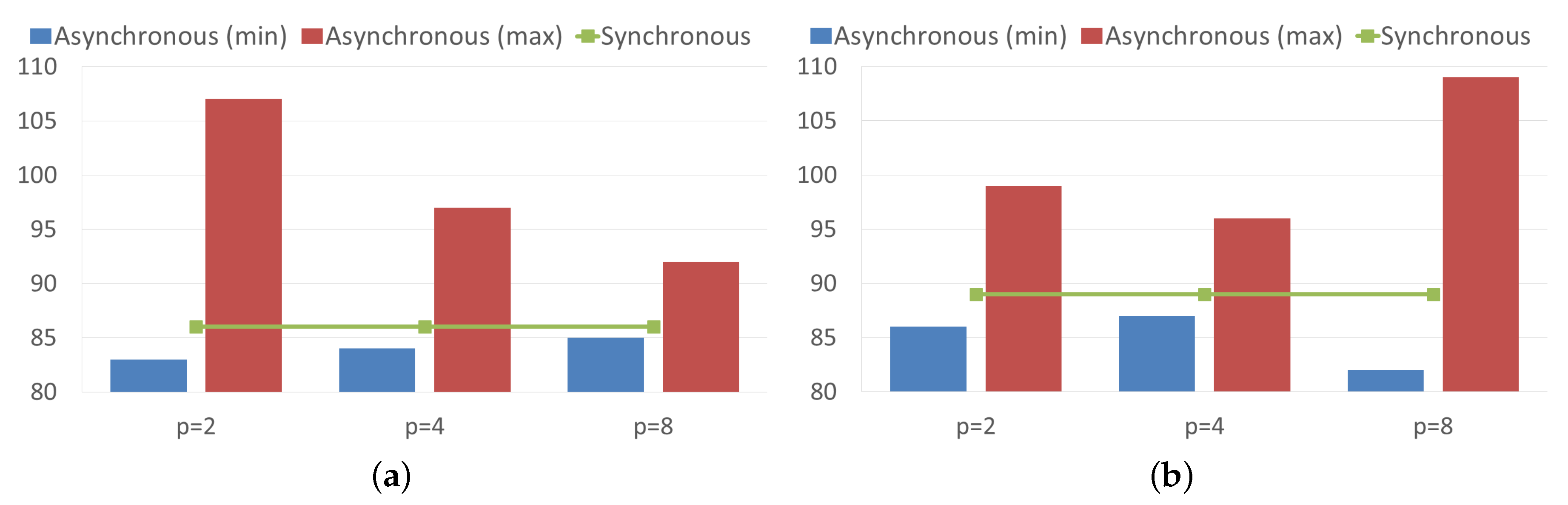Figure 1 compares the needed iterations for reaching convergence with both the synchronous and asynchronous Power algorithms. For this purpose, the asynchronous algorithm was executed three times, and the maximum and minimum number of iterations across processes are reported in this figure. As it can be seen, the number of synchronous iterations needed for convergence of the Power method for the analyzed matrices is similar, 86 iterations for the uk-2002 matrix and 89 iterations for the it-2004 matrix. In the asynchronous case, each process performs a different number of iterations. Then, although some processes perform a number of local iterations less than the number of iterations of the synchronous model, the number of local iterations performed for the slower process increases degrading the performance. This is consistent with some observations done in previous works [34,35] about the interest of the asynchronous algorithms for load unbalanced problems or for problems executed in a heterogeneous parallel computing system, while these asynchronous model are not always advantageous for well-balanced problems like ours.

In the rest of the experiments reported here, we used $ϵ={10}^{-6}$, for the stopping criterion and we have run our algorithms for several values of $\alpha$.

Taking into account that the work among nodes has been balanced by means of the above explained nonzero element distribution, the best strategy for designing the parallel algorithms proposed here is the one that keeps this load balancing. Therefore, at each global iteration of the algorithm, every block of the iterate vector must be updated the same number of times before all processes synchronize to get a new global iterate. However, in the hypothetical case in which the node workload may be unbalanced or when working on a heterogeneous parallel computing system, the designed algorithms allow us to perform different number of updates for each block of the iterate vector avoiding the downtime of any of the nodes and leading to a better load balancing in the parallel algorithms. 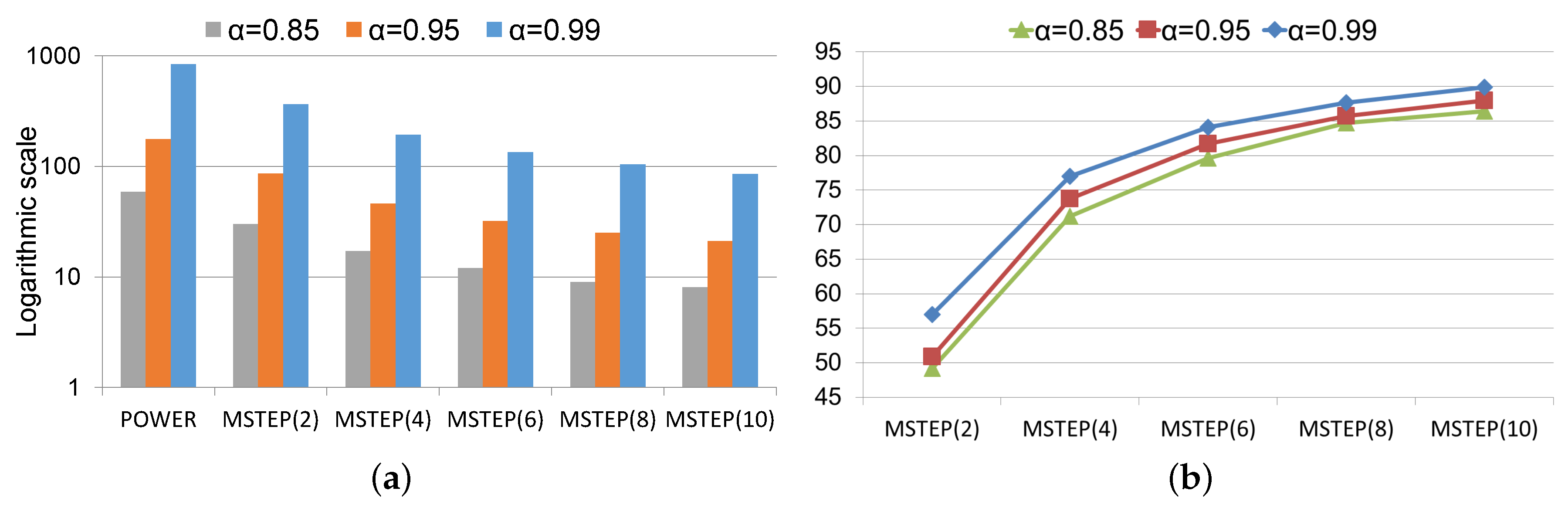Figure 2 illustrates the behaviour of the convergence rates of the Power method and the MSTEP methods for the uk-2002 matrix and setting $\alpha =0.85$, $0.95$, and $0.99$. The notation MSTEP(q) indicates that, at each global iteration, each vector block i is updated $q(i)=q$ times in the algorithm before synchronizing.

Note that the synchronization points in the MSTEP methods are reduced in relation to the Power method as q increases. However, in this algorithm, actualizing a certain number of times each block of vector without waiting for the update of other parts of the global iterate vector, is more computationally intense than applying one iteration of the Power method. As long as this overhead is minimal, the proposed acceleration is beneficial. 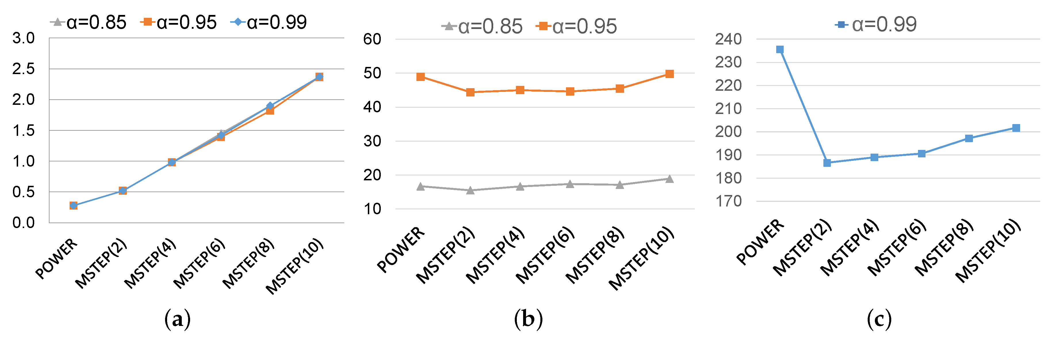In order to show this, Figure 3 displays the comparison of times (per iteration and total time) between the Power method and the MSTEP algorithm for several values of q. As it can be seen in Figure 3, the values of q must be kept small. The best choices of q are obtained for q between 2 and 4. Particularly, using 4 cores in shared memory, the MSTEP algorithm achieves a gain in relation to the parallel Power method up to $21\%$ for the smallest matrix of our dataset.

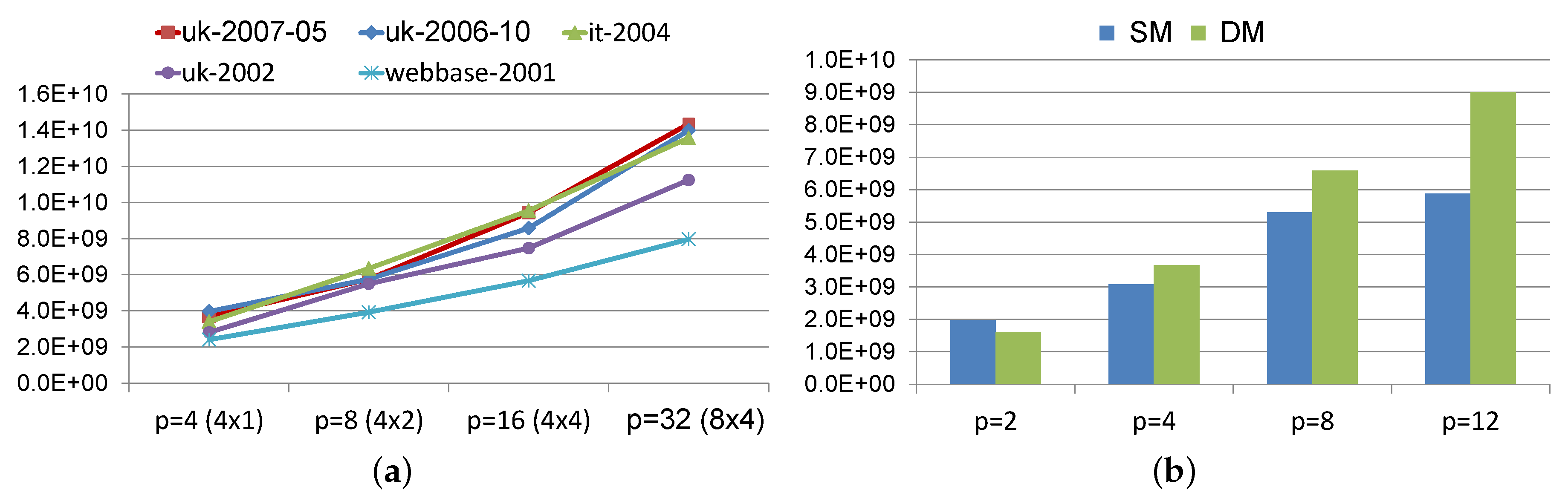
Figure 4 compares the floating-point operations per second (Flops) accomplished by this algorithm using different configurations of processes. Even though an acceptable performance is obtained using the 12 available cores of one node, it is not comparable with the performance obtained using distributed memory or a hybrid scheme.

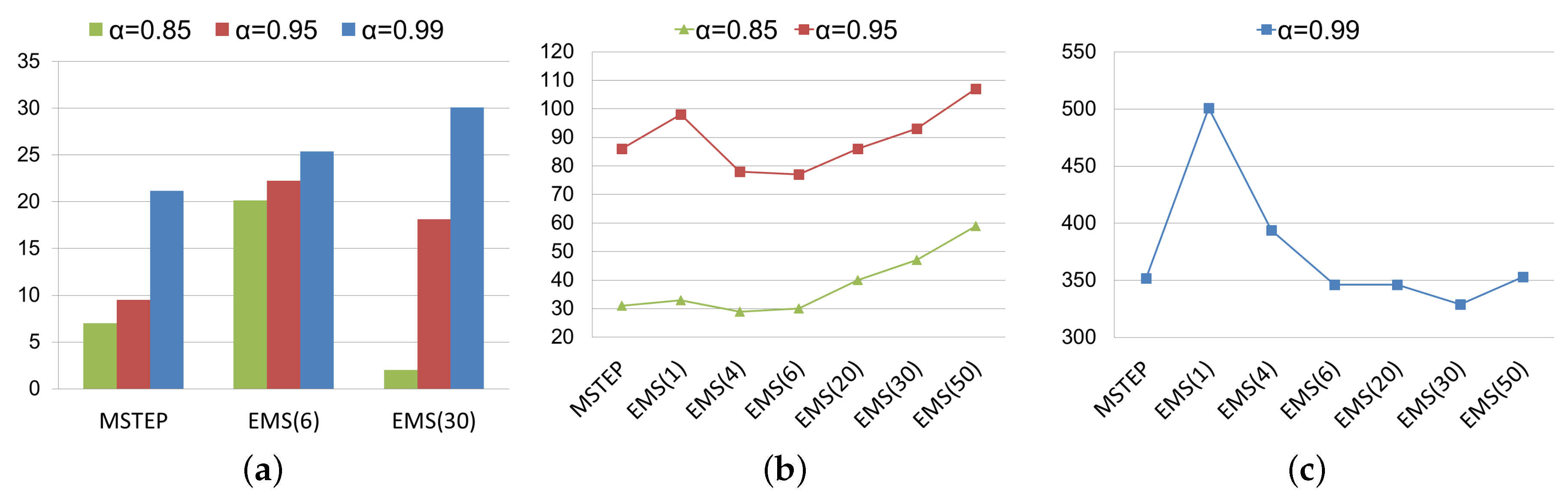
Figure 5 analyzes the effect of performing the extrapolation before running the non-stationary iterations, that is the EMS algorithm is considered. The notation EMS(r) indicates the value of r used for the extrapolation. As it is expected, simple extrapolation ($r=1$) is not effective. This makes sense because, from a theoretical point of view, a simple extrapolation assumes that $\alpha$ is the only eigenvalue of modulus $\alpha$ and this is inaccurate. In fact, it is known that the use of the simple extrapolation technique ($r=1$) in the Power method slows down its convergence [36]. On the other hand, the choice of r in our algorithm depends on the condition number of the problem. Given our experience with the EMS algorithm, while for a well-conditioned problem a good choice for r is $r=6$, it should be chosen greater than 6 when $\alpha \to 1$, obtaining generally a good strategy by choosing $r=30$.

To analyze the effectiveness of the proposed parallel algorithms, we have also compared them with the inner-outer Power algorithm (In-out) proposed in Reference [15], the parallel extrapolation algorithms (EXT and RELEXT) proposed in Reference [18], and the parallel two-stage algorithms (LTW and extrapolated LTW) designed in Reference [20].

In order to compare these algorithms, their parallel implementations have been developed using the same $mCSR$ storage format as in the algorithms treated in this work. Furthermore, the parallel implementations of these methods have also been developed using a hybrid MPI/OpenMP scheme and the same matrix distribution strategy. We would like to point out that the OpenMP code proposed in [15] was analyzed using 8 cores. Also, the Web graphs used for showing its performance were compressed into bvgraph compression schemes [37]. However, as we showed in a previous work [20], the compression scheme used in Reference [15] causes $4-8x$ slowdown with respect to the $mCSR$ storage format, being the $mCSR$ storage format much more efficient for computing the PageRank vector.

Figure 6 compares the gain obtained by both the non-stationary and the inner-outer Power methods in relation to the parallel Power method. This figure includes the relaxed version of the EMS algorithm, called RELEMS algorithm. Good choices of the relaxation parameter $\beta$, in this algorithm, are between $0.98$ and $0.99$. As this figure shows, the parallel algorithms treated herein accelerate the computation of the PageRank vector more significantly than the parallel inner-outer Power algorithm. In fact, for $\alpha =0.99$ and using 32 processes, the inner-outer Power algorithm achieves a gain in relation to the parallel Power method between $5.21\%$ and $35.86\%$ while the achieved gain by means of the RELEMS algorithm was between $31.17\%$ and $58.38\%$.

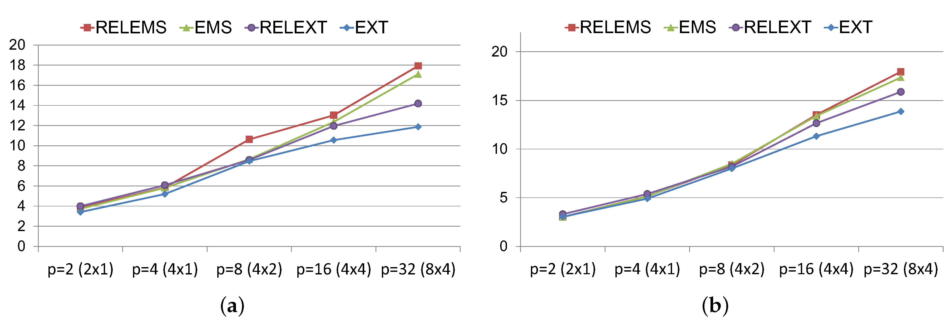
Figure 7 analyzes the global speedups achieved for the extrapolated non-stationary algorithms with respect to those obtained for the EXT and RELEXT algorithms from [18], setting the sequential Power method as reference algorithm. Notice that, using a number less than or equal to 8 processes, similar efficiencies are obtained. However, the non-stationary algorithms outperform, more sharply, both the EXT and RELEXT algorithms as the number of processes increases and, therefore, the number of needed communications among processes. In this sense (see Figure 7), the non-stationary algorithms have accelerated the convergence time in relation to the sequential Power algorithm up to 14 times using 4 nodes and 4 OpenMP threads per node, and up to 18 times using 8 nodes with the same thread configuration.

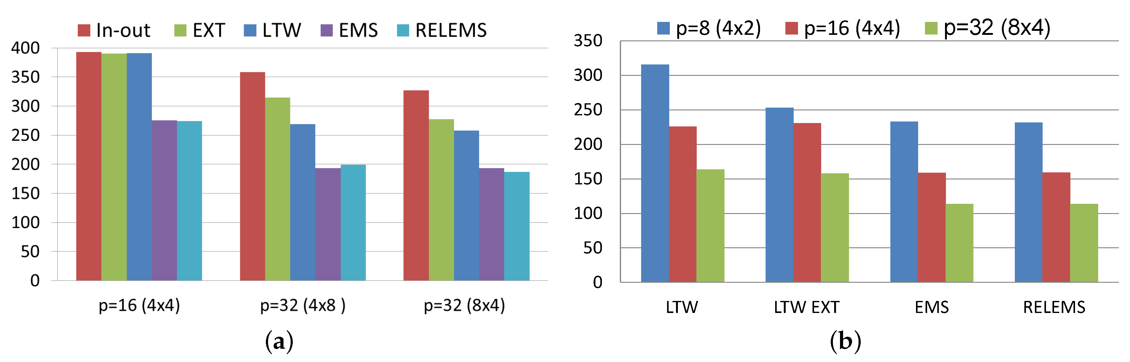
Figure 8 compares the algorithms developed in this work, EMS and RELEMS algorithms, with the parallel two-stage algorithms designed in [20] for solving PageRank, called LTW algorithm and its extrapolated version (LTW EXT). As it can be seen in Figure 8a, the best parallel two-stage algorithm also outperforms the inner-outer and the extrapolated Power algorithms as the number of processes increases. Nevertheless the gains achieved with these methods are not comparable with those obtained with the proposed EMS and RELEMS algorithms. So, the parallel non-stationary algorithms obtain a reduction time of up to $37\%$ in relation to the best (extrapolated or non-extrapolated) parallel two-stage algorithm, when setting $\alpha =0.98$.

5. Conclusions

In this paper, using the eigenvector formulation of PageRank, a non-stationary technique based on the Power method for the parallel computation of PageRank was proposed and its convergence established. For theoretically ensuring the global convergence of the proposed parallel non-stationary algorithms, we have shown that the designed non-stationary technique can be seen as a particular case of asynchronous algorithm in which the involved parameters have been constructed satisfying sufficient conditions for such convergence. The parallel implementations of several strategies combining this technique and the extrapolation methods have been developed using a hybrid MPI/OpenMP model. The MSTEP algorithm has been designed using the basic parallel non-stationary Power method, while the EMS algorithm is a particular case of the parallel non-stationary algorithms in which an initial vector nearest to the solution is previously obtained. This vector is obtained using once the extrapolation technique. Additionally, the RELEMS algorithm corresponds to the relaxed counterpart of the EMS algorithm.

For validating the proposed algorithms, we used different datasets, publicly available from the Laboratory for Web Algorithmics [31]. Taking into account the characteristics of the transition matrices, a modified Compressed Sparse Row format has been used involving a considerable reduction of memory requirements with respect to the popular $CSR$ format of up to $73\%$. In order to balance the calculations among nodes, a nonzero elements partitioning is used, obtaining empirically that, in order to keep this load balancing, every block of the iterate vector must be locally updated the same number of times (q) before constructing the next global iterate. Moreover, the best non-stationary algorithms were obtained using a small q between 2 and 4.

By comparing the proposed parallel non-stationary algorithms, the best results have been obtained with the EMS and RELEMS algorithms, choosing $r=6$ as the parameter involved in the extrapolation for well-conditioned problem (e.g., using $\alpha =0.85$) and greater than 6 when the damping factor $\alpha$ is closer to 1. Moreover, good choices for the relaxation parameter of the RELEMS algorithm are between $\beta =0.98$ and $\beta =0.99$.

Lastly, but not least important, the numerical results analyzed in this work show the good behaviour of the parallel non-stationary algorithms compared with some well-known techniques used for computing PageRank such as the parallel extrapolation algorithms studied in Reference [18], the inner-outer Power algorithm proposed in Reference [15], and the parallel two-stage algorithms designed in Reference [20], obtaining gains of up to $58.4\%$ in relation to the parallel Power algorithm.