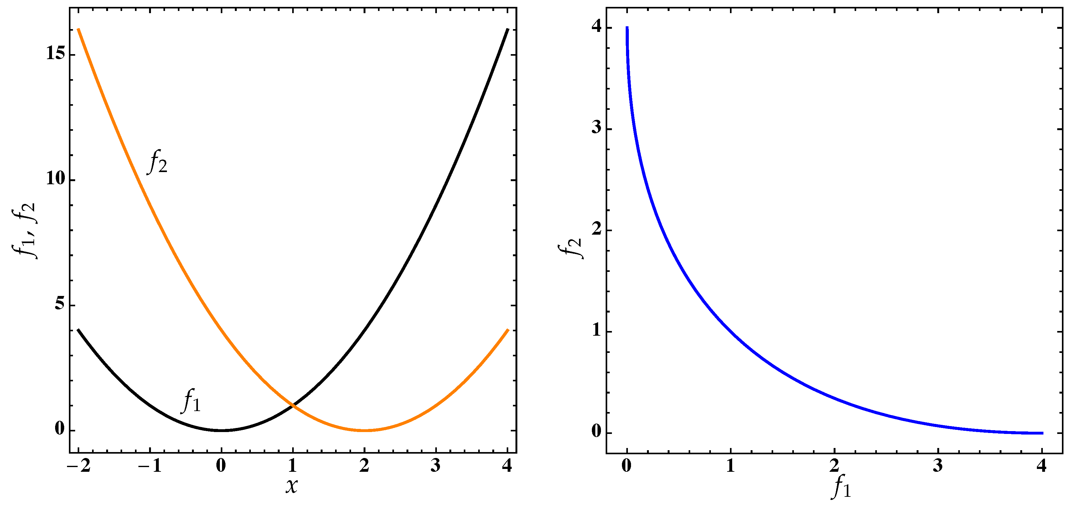
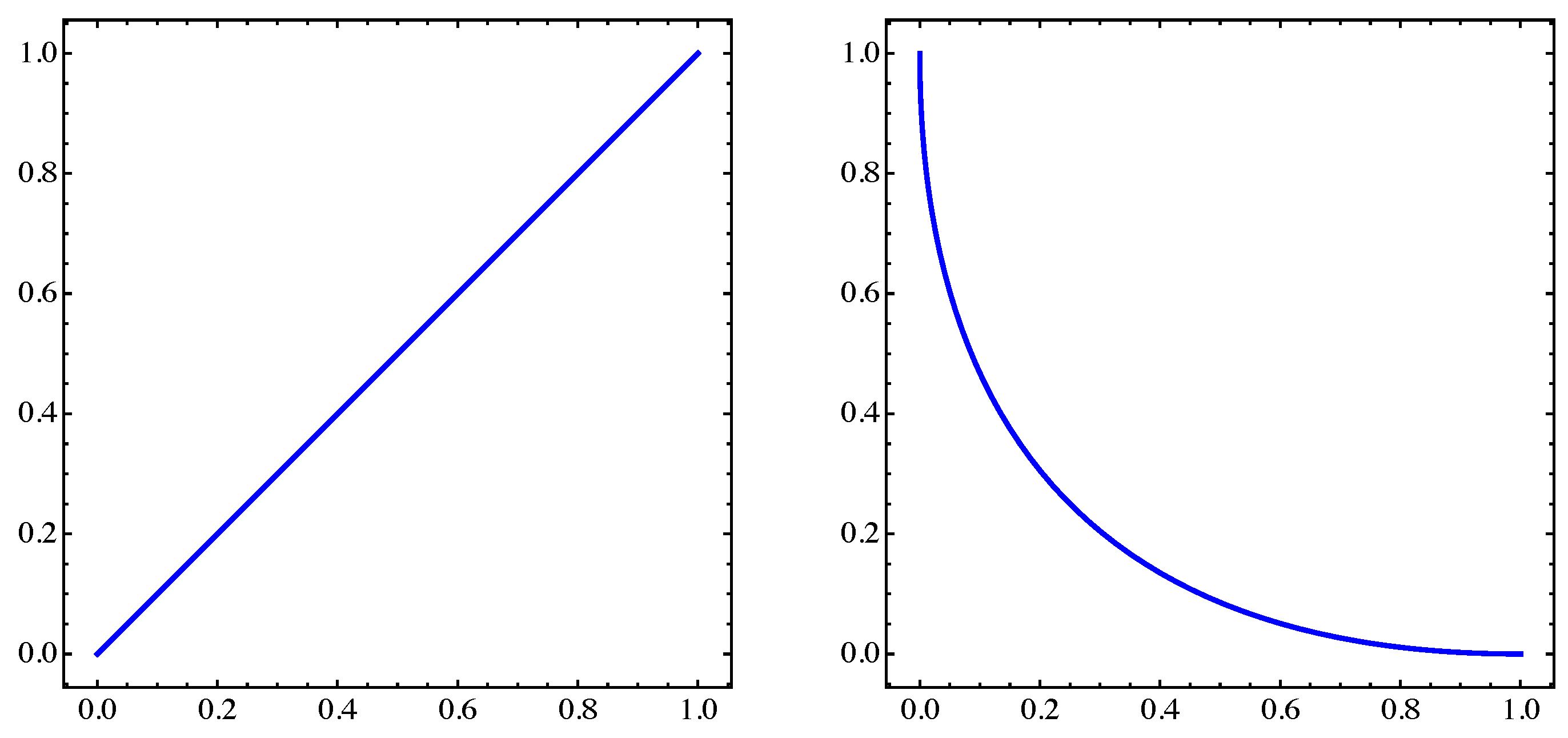
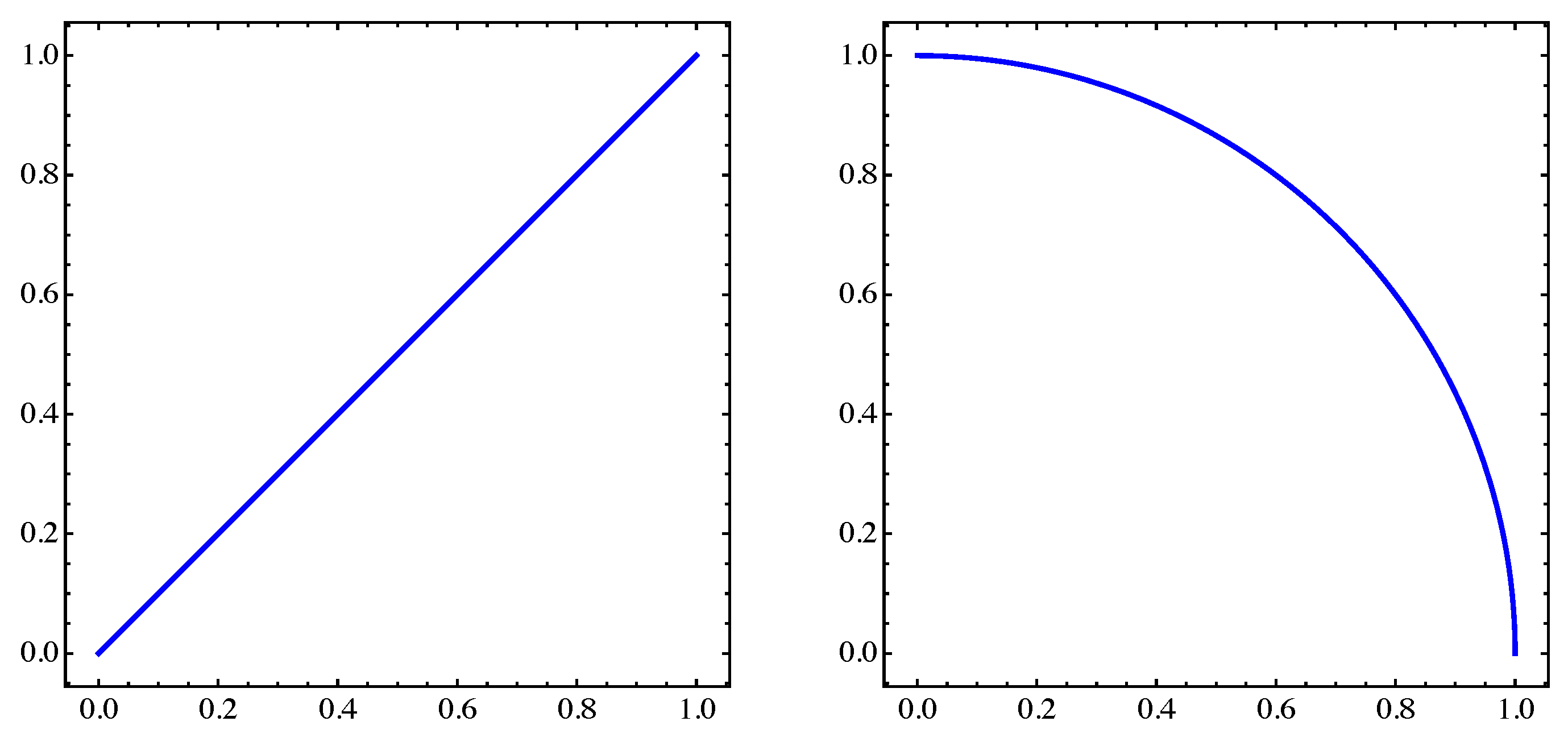
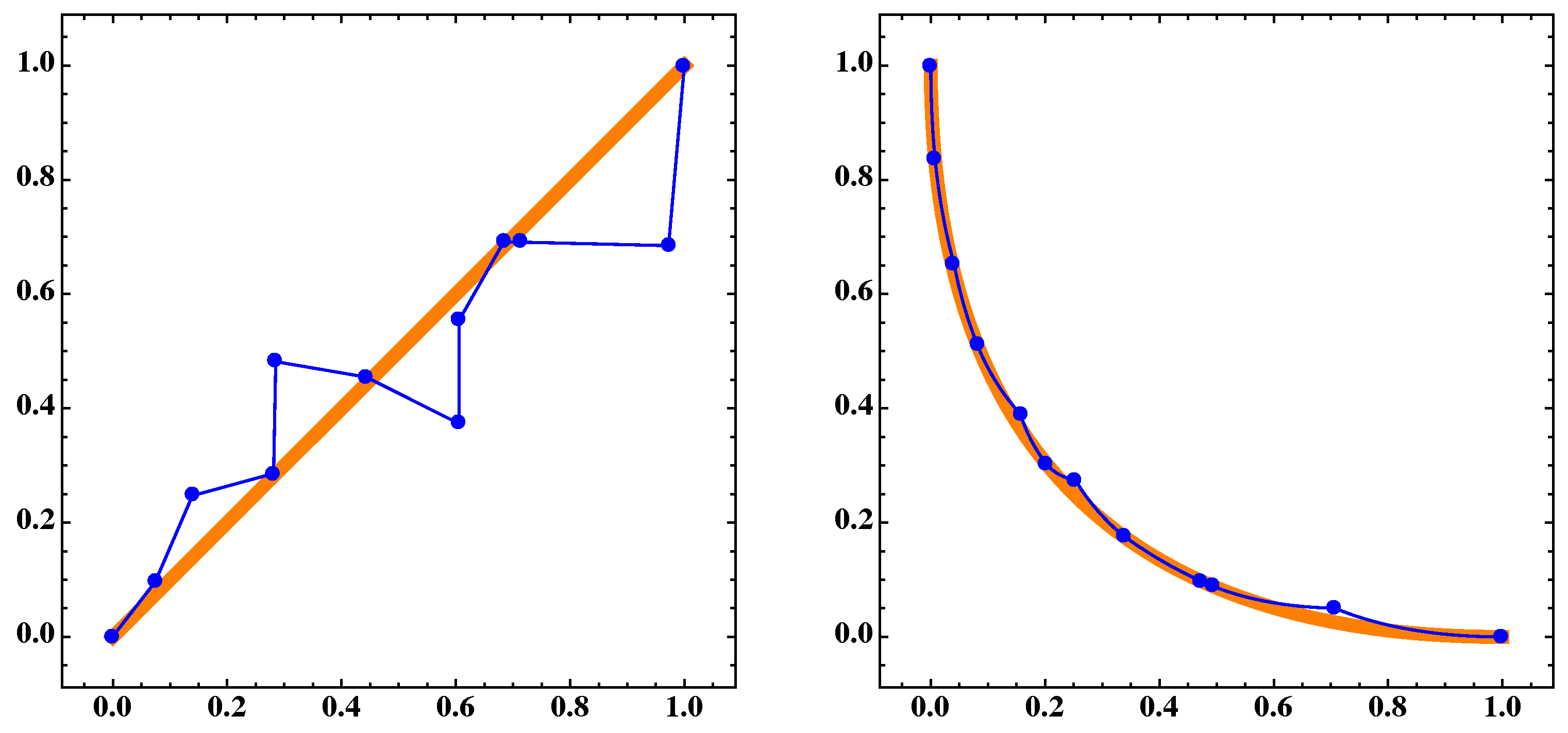
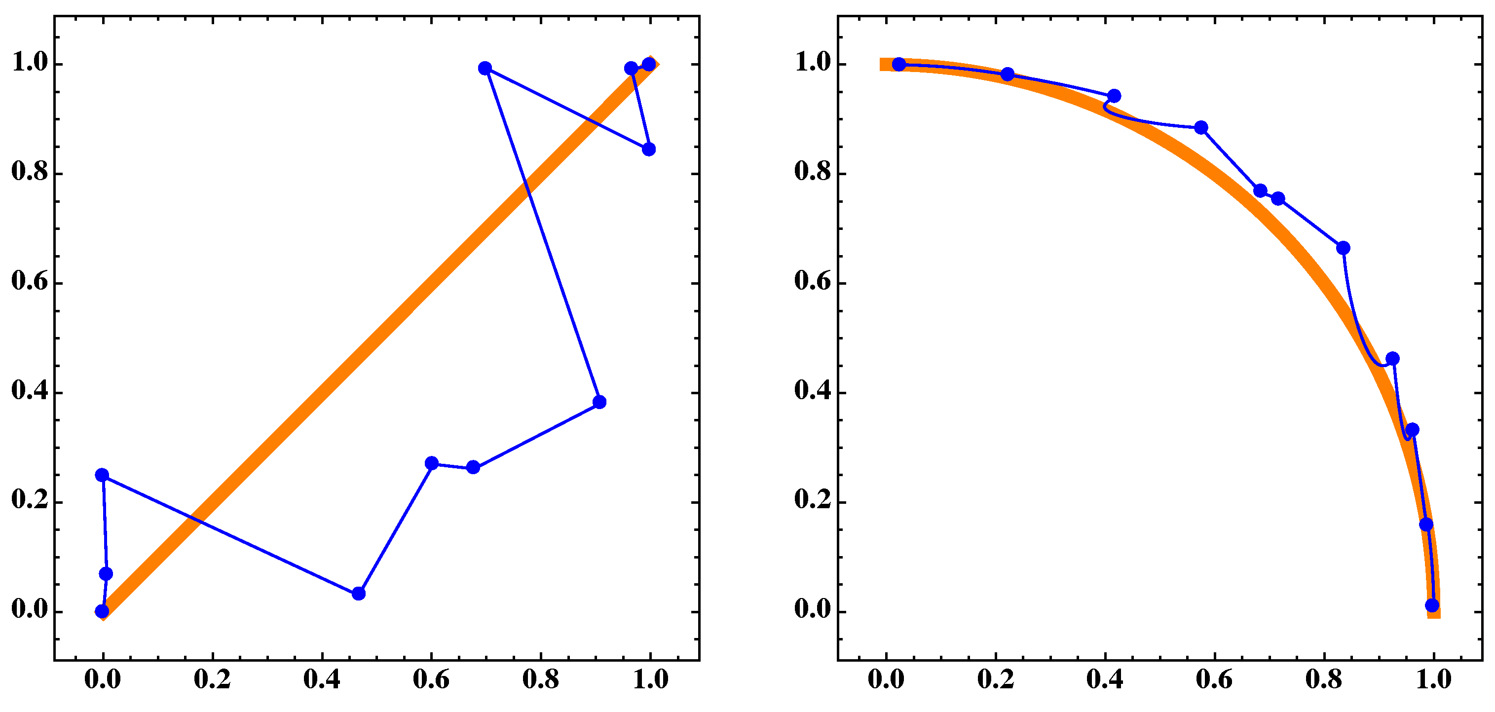
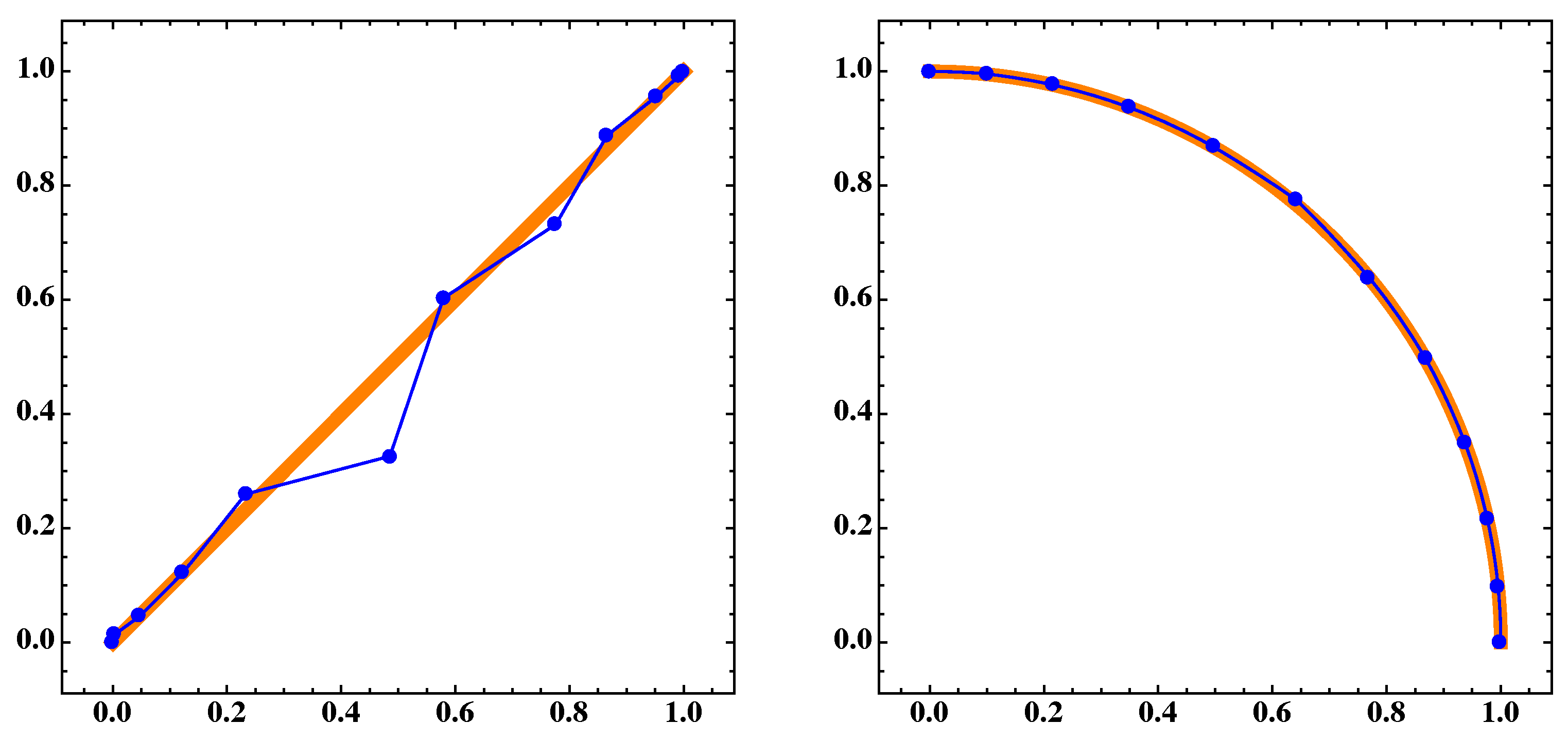
Figure 1.
Left: the objectives
and
from a multi-objective optimization problem (MOP; Equation (
1)).
Right: the corresponding Pareto set over the interval
.
Figure 1.
Left: the objectives
and
from a multi-objective optimization problem (MOP; Equation (
1)).
Right: the corresponding Pareto set over the interval
.
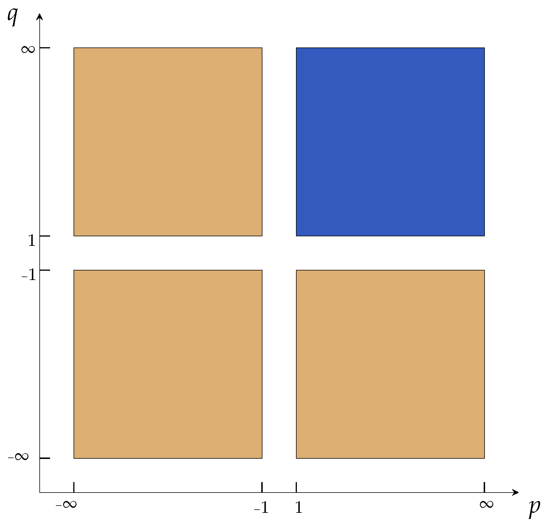
Figure 2.
According to Corollary 1, when acting on disjoint subsets, behaves as a proper metric if lies in the blue sector, and according to Corollary 2, it behaves like an inframetric if lies in the orange sectors.
Figure 2.
According to Corollary 1, when acting on disjoint subsets, behaves as a proper metric if lies in the blue sector, and according to Corollary 2, it behaves like an inframetric if lies in the orange sectors.
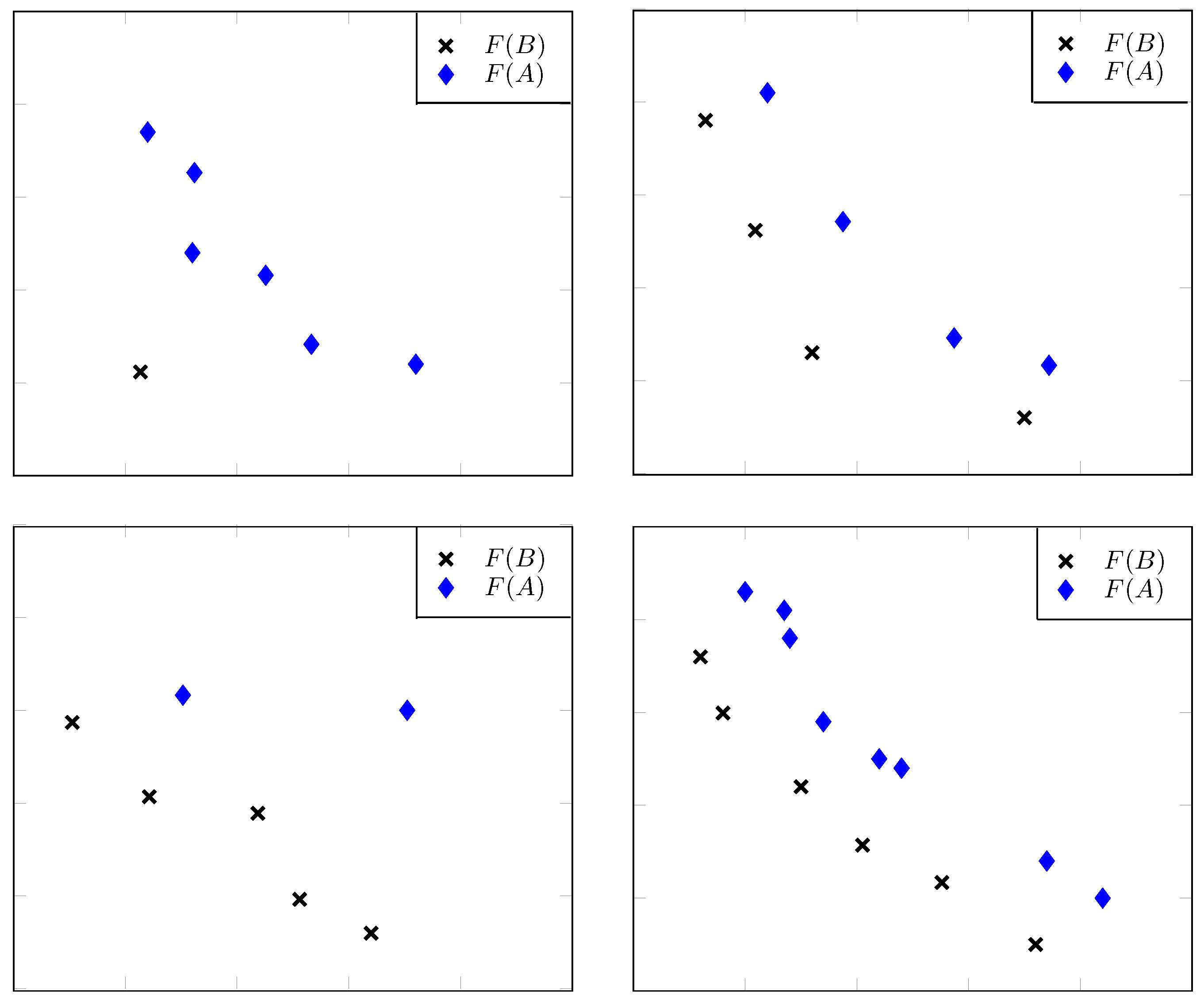
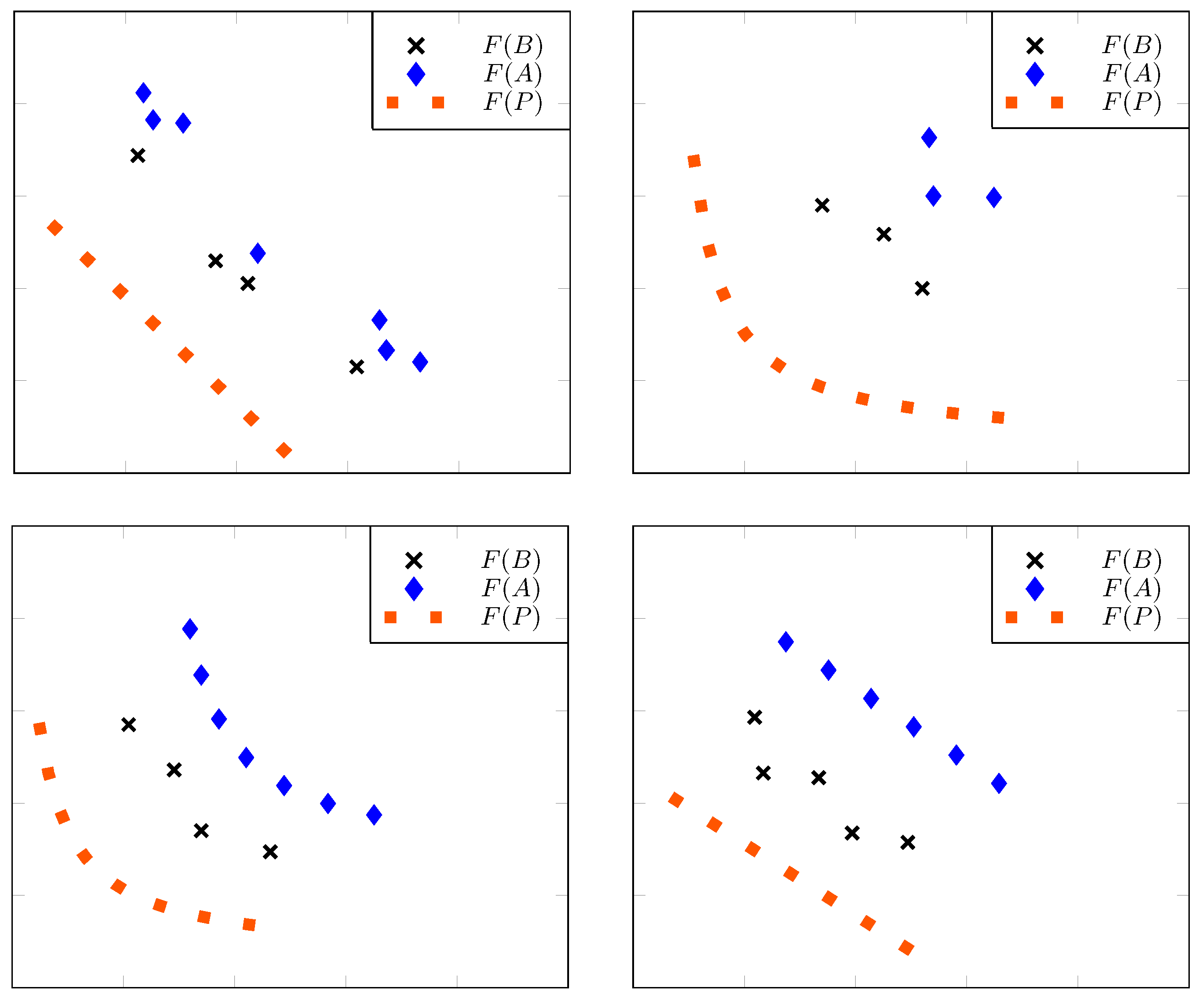
Figure 3.
Different scenarios where the value of archive B is better (smaller) than the value of archive A independently of the Pareto set and where the additional assumptions made in Theorem 5 are easily verifiable.
Figure 3.
Different scenarios where the value of archive B is better (smaller) than the value of archive A independently of the Pareto set and where the additional assumptions made in Theorem 5 are easily verifiable.
Figure 4.
Two situations where is better (smaller) than for sufficiently negative q: Here, the hypotheses of Proposition 3 hold true.
Figure 4.
Two situations where is better (smaller) than for sufficiently negative q: Here, the hypotheses of Proposition 3 hold true.
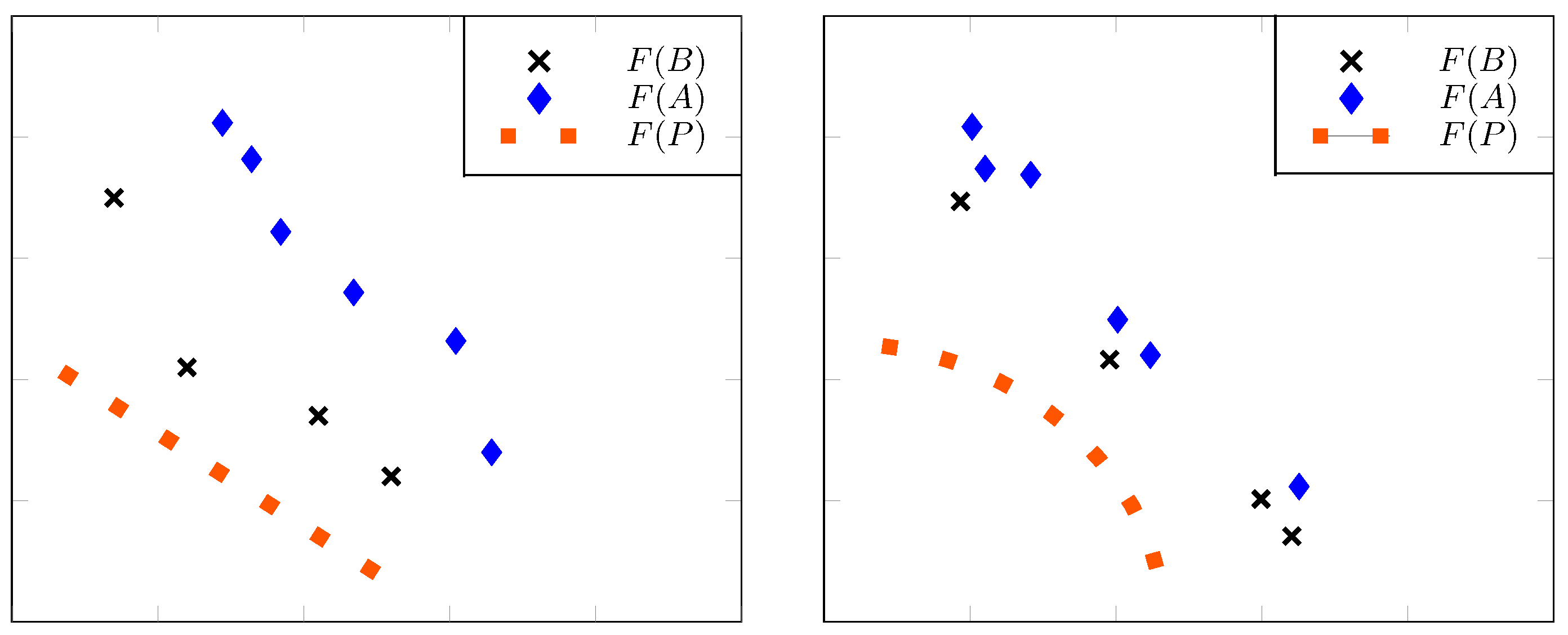
Figure 5.
Four examples where is smaller (better) than for sufficiently negative q: In each case, at least one of the requirements of Theorem 6 is satisfied.
Figure 5.
Four examples where is smaller (better) than for sufficiently negative q: In each case, at least one of the requirements of Theorem 6 is satisfied.
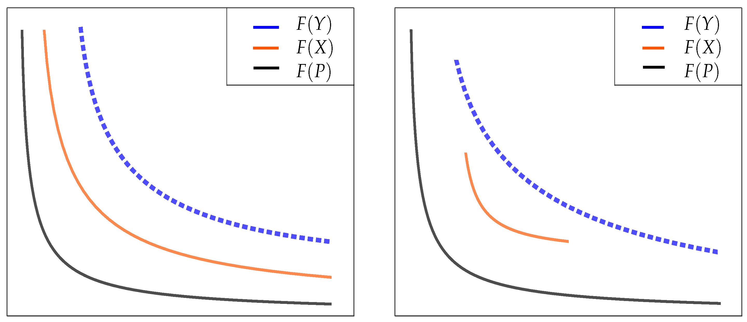
Figure 6.
(Left) A situation where the Pareto front and the images and of continuous archives satisfy and condition 1(a) of Theorem 8 holds true. (Right) A modification of the previous situation where conditions and of Remark 6 are satisfied but . Here, there are no possible partitions of the archives satisfying part 1(a) of Theorem 8.
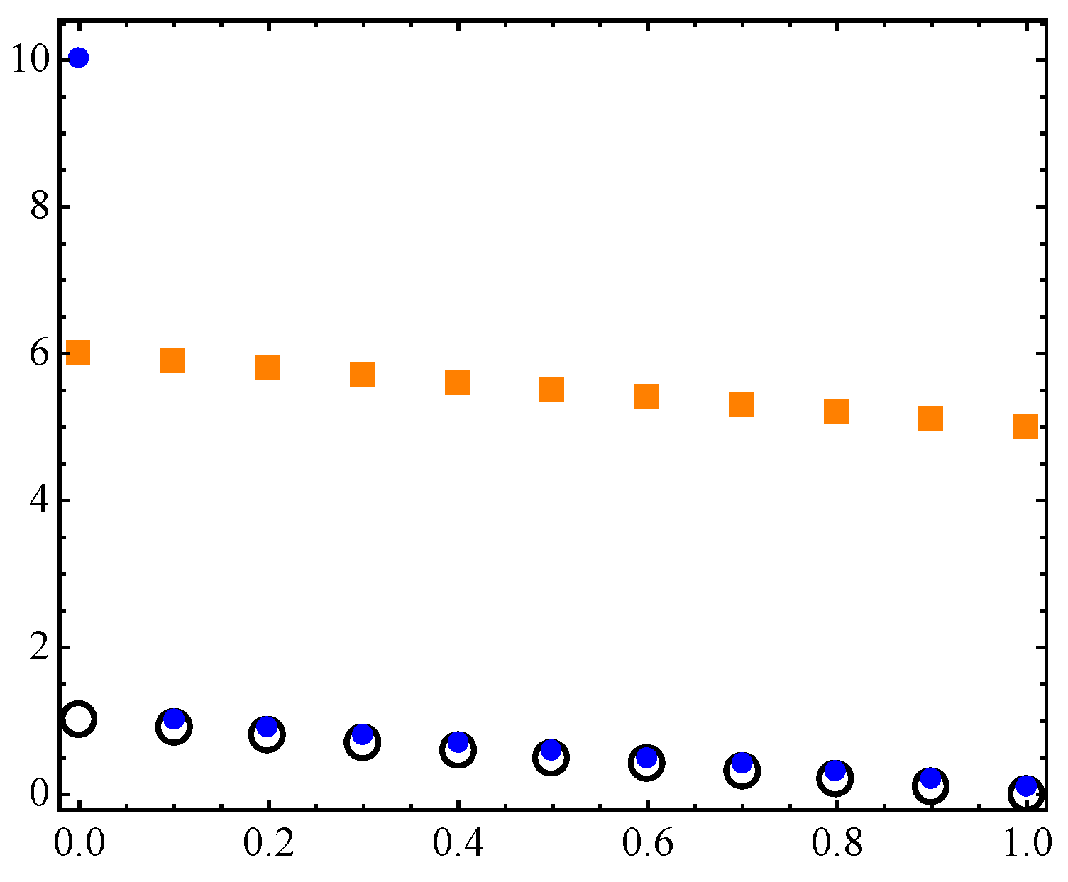
Figure 7.
A hypothetical Pareto front discretization (black circles) and two different archives: (blue dots) and (orange squares).
Figure 7.
A hypothetical Pareto front discretization (black circles) and two different archives: (blue dots) and (orange squares).
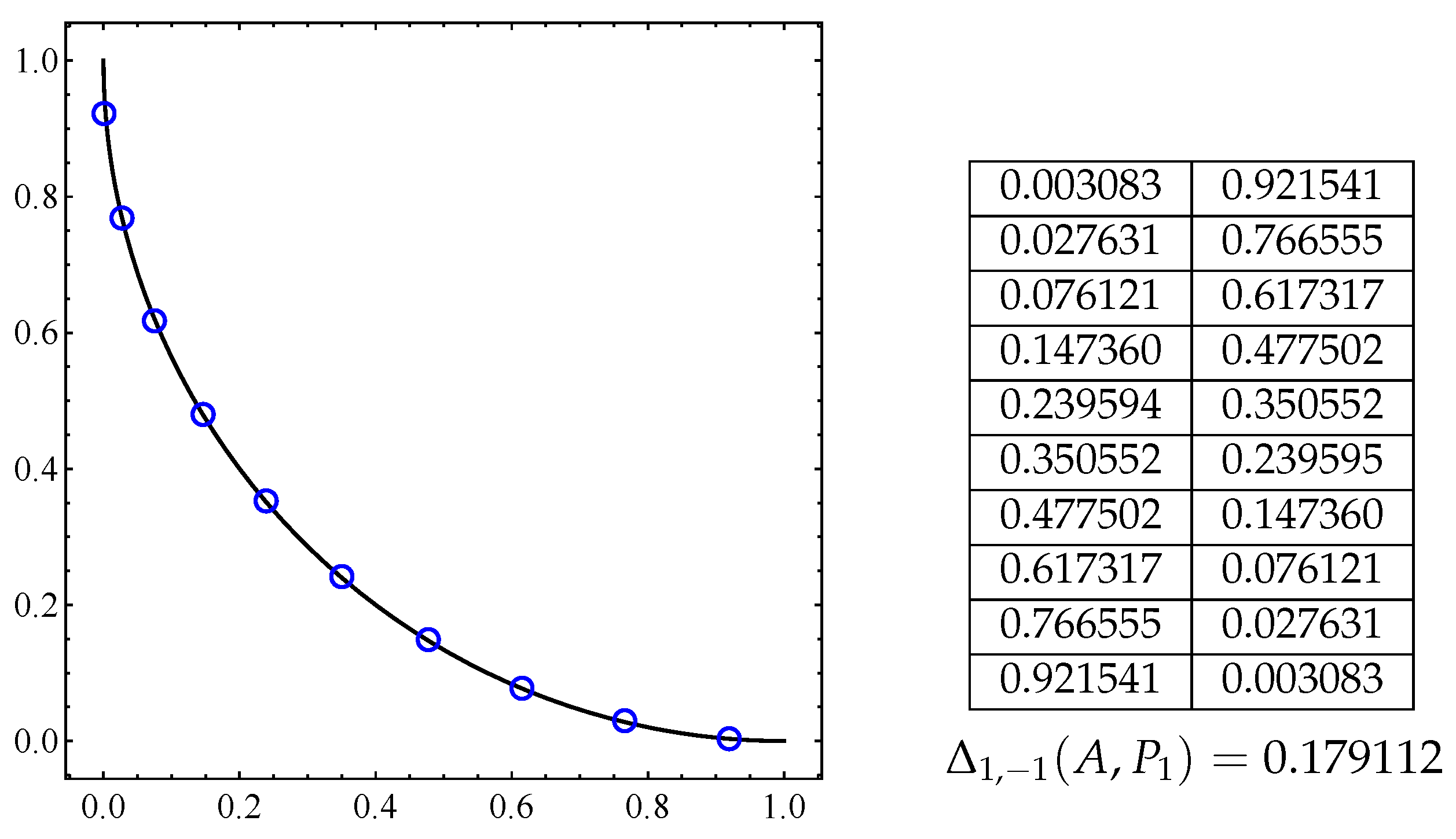
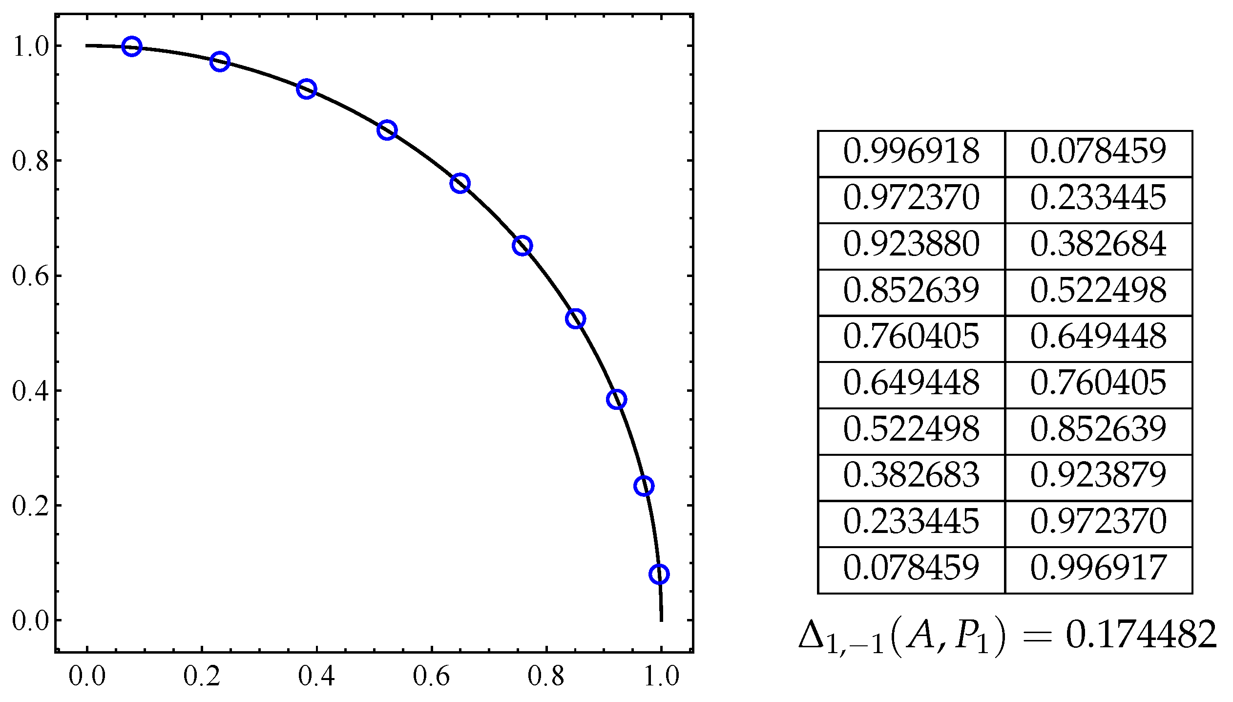
Figure 8.
Optimal archive A for the connected Pareto front given by Equation (12) with 10 elements (blue circles) and at the right is the respective archive coordinates and the distance.
Figure 8.
Optimal archive A for the connected Pareto front given by Equation (12) with 10 elements (blue circles) and at the right is the respective archive coordinates and the distance.
Figure 9.
Optimal archive A for the connected Pareto front given by Equation (12) with 10 elements (blue circles) and at the right is the respective archive coordinates and the distance.
Figure 9.
Optimal archive A for the connected Pareto front given by Equation (12) with 10 elements (blue circles) and at the right is the respective archive coordinates and the distance.
Figure 10.
Optimal five-point set archives A for the connected Pareto front given by Equation (12) with and .
Figure 10.
Optimal five-point set archives A for the connected Pareto front given by Equation (12) with and .
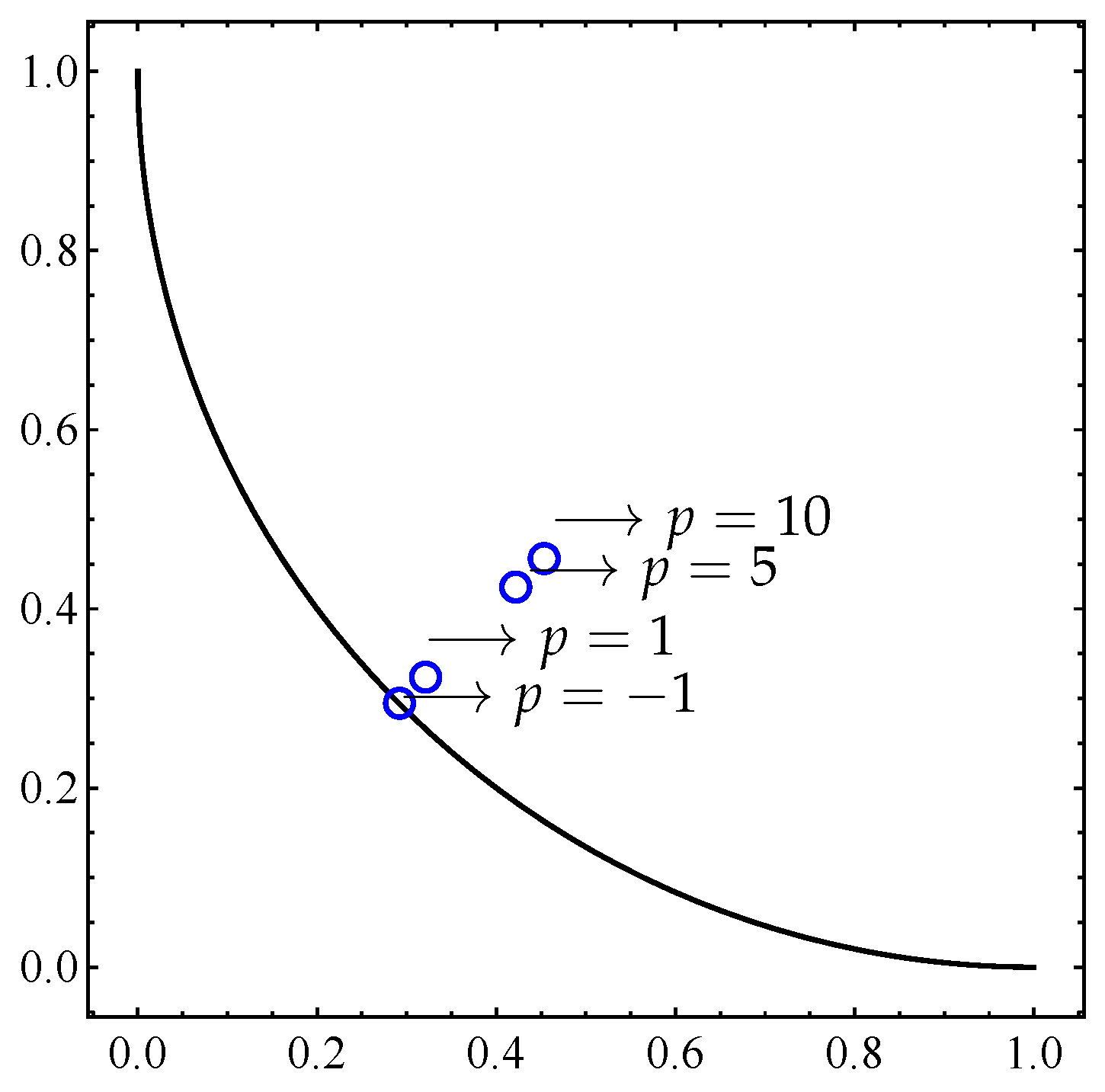
Figure 11.
Optimal one-point archives A for the connected Pareto front given by Equation (12) with and different values of p: In all cases, the archives are located in the line .
Figure 11.
Optimal one-point archives A for the connected Pareto front given by Equation (12) with and different values of p: In all cases, the archives are located in the line .
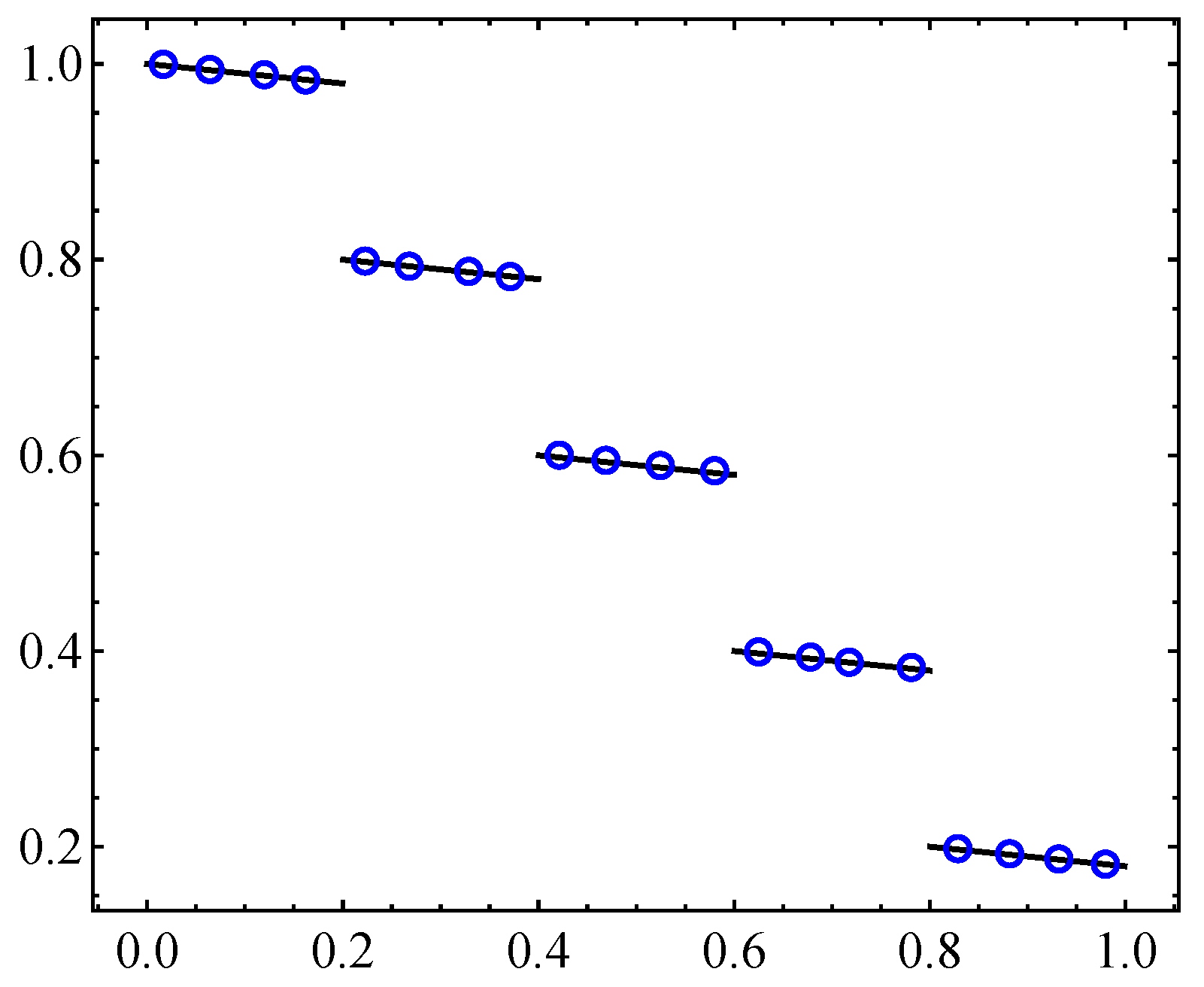
Figure 12.
Numerical optimal archive A for the disconnect step Pareto front given by Equation (13) with 20 elements: here, we obtain .
Figure 12.
Numerical optimal archive A for the disconnect step Pareto front given by Equation (13) with 20 elements: here, we obtain .
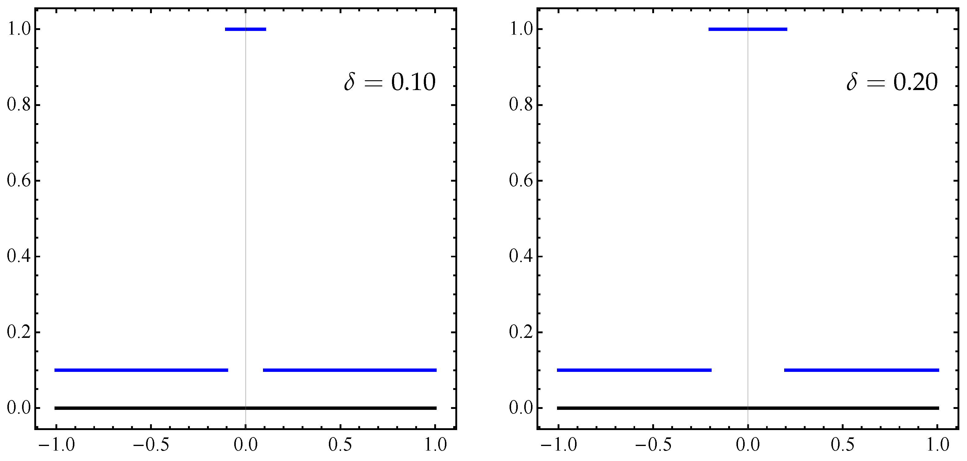
Figure 13.
The black horizontal segment is the set A from Equation (14), and the blue piecewise map is the respective approximation given by the set from Equation (15) for two values of and .
Figure 13.
The black horizontal segment is the set A from Equation (14), and the blue piecewise map is the respective approximation given by the set from Equation (15) for two values of and .
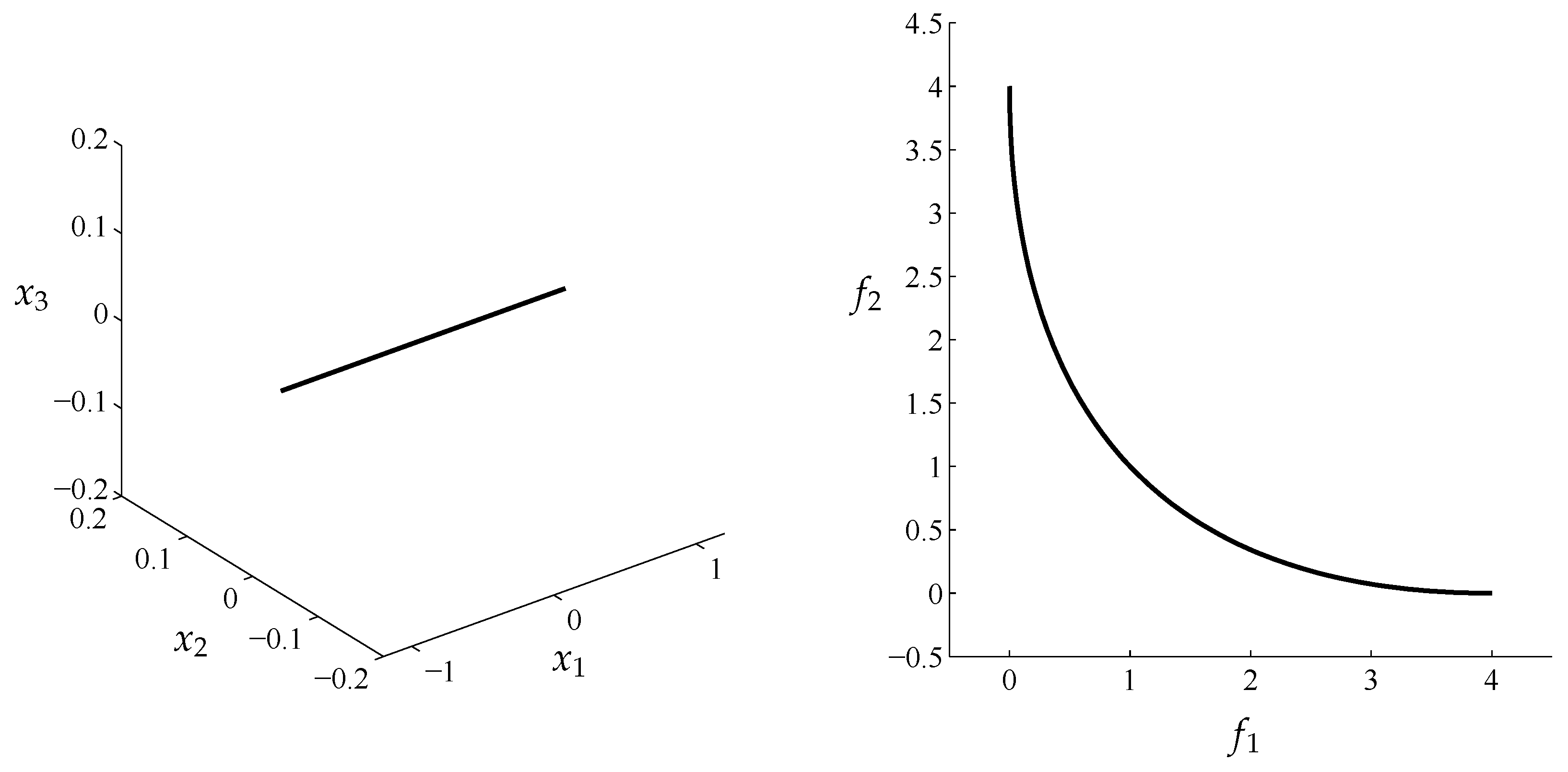
Figure 14.
(Left) Pareto set. (Right) Pareto front of MOP (Equation (16)) for and .
Figure 14.
(Left) Pareto set. (Right) Pareto front of MOP (Equation (16)) for and .
Figure 15.
The same as in
Figure 14 but for
.
Figure 15.
The same as in
Figure 14 but for
.
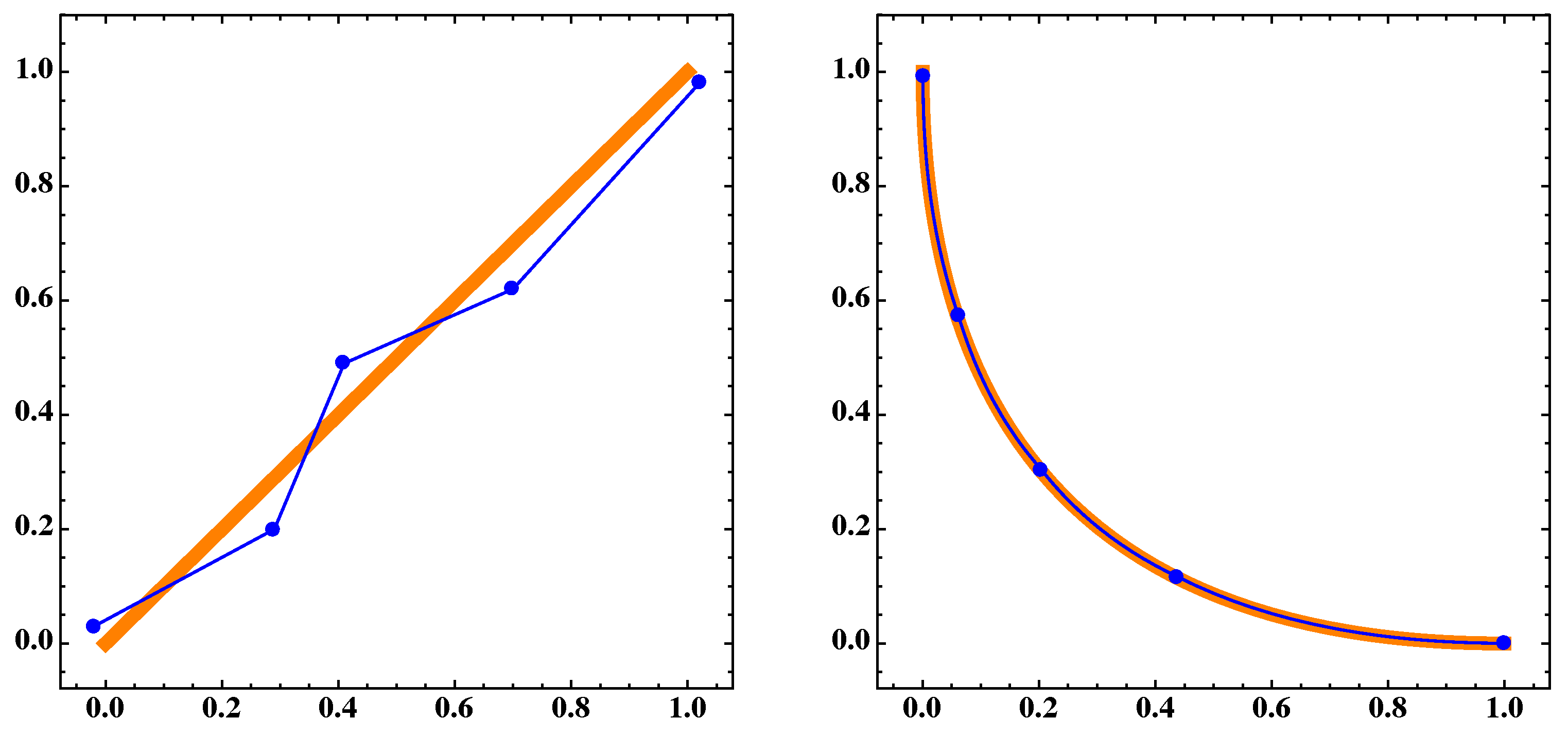
Figure 16.
(Left) The blue dots A and the blue polygonal line B are the discrete and continuous approximations, respectively, for the Pareto set which corresponds to the orange thick segment, of MOP (Equation (16)) for . (Right) respective sets and of the Pareto front for .
Figure 16.
(Left) The blue dots A and the blue polygonal line B are the discrete and continuous approximations, respectively, for the Pareto set which corresponds to the orange thick segment, of MOP (Equation (16)) for . (Right) respective sets and of the Pareto front for .
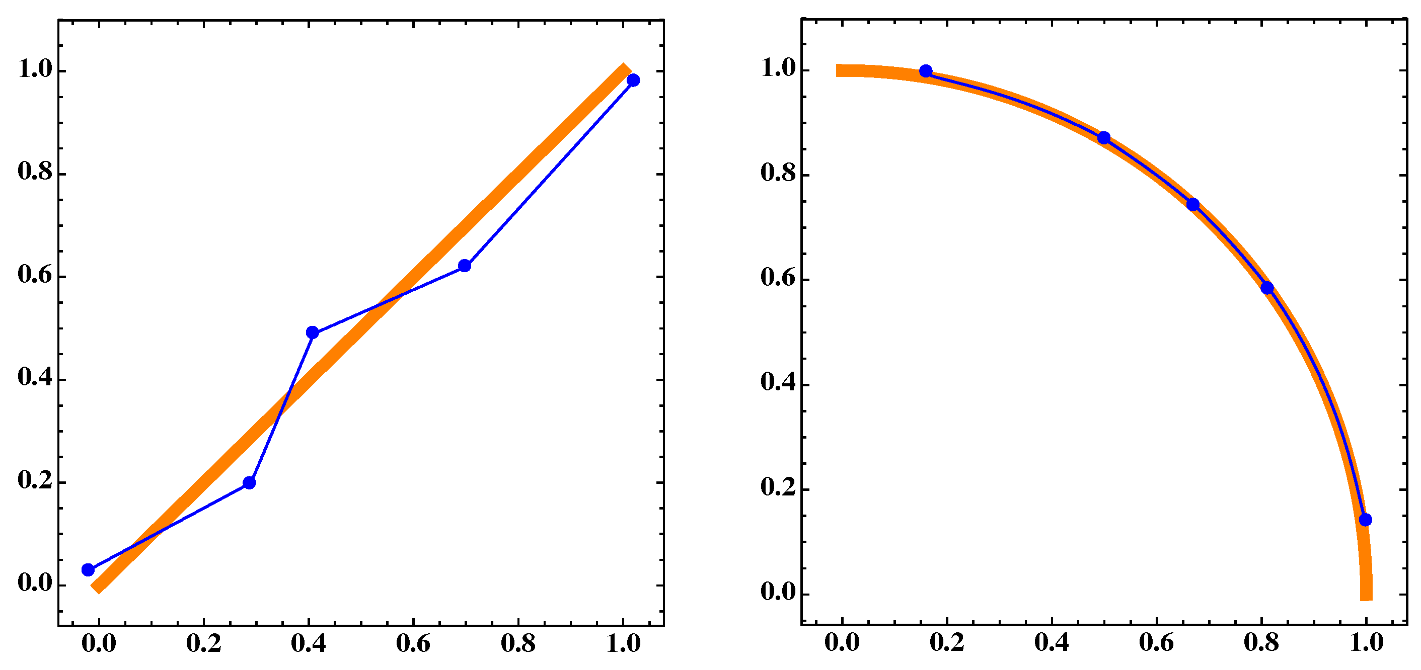
Figure 17.
The same as in
Figure 16 but for
.
Figure 17.
The same as in
Figure 16 but for
.
Figure 18.
(Left) the blue dots A and the blue polygonal line are the discrete and continuous approximations, respectively, for the Pareto set and the orange thick segment is for the 410th generation of the NSGA-II algorithm of MOP (Equation (16)) for . (Right) corresponding sets and of the Pareto front for .
Figure 19.
The same as in
Figure 18 but for
.
Figure 19.
The same as in
Figure 18 but for
.
Figure 20.
(
Left) the blue dots
A and the blue polygonal line are the discrete and continuous approximations, respectively, for the Pareto set and the orange thick segment is for the 410th generation of the MOEA/D algorithm of MOP (Equation (
17)) for
. (
Right) corresponding sets
and
of the Pareto front for
.
Figure 21.
The same as in
Figure 20 but for
.
Figure 21.
The same as in
Figure 20 but for
.
Figure 22.
(Left) Pareto set. (Right) Pareto front of MOP (Equation (17)).
Figure 22.
(Left) Pareto set. (Right) Pareto front of MOP (Equation (17)).
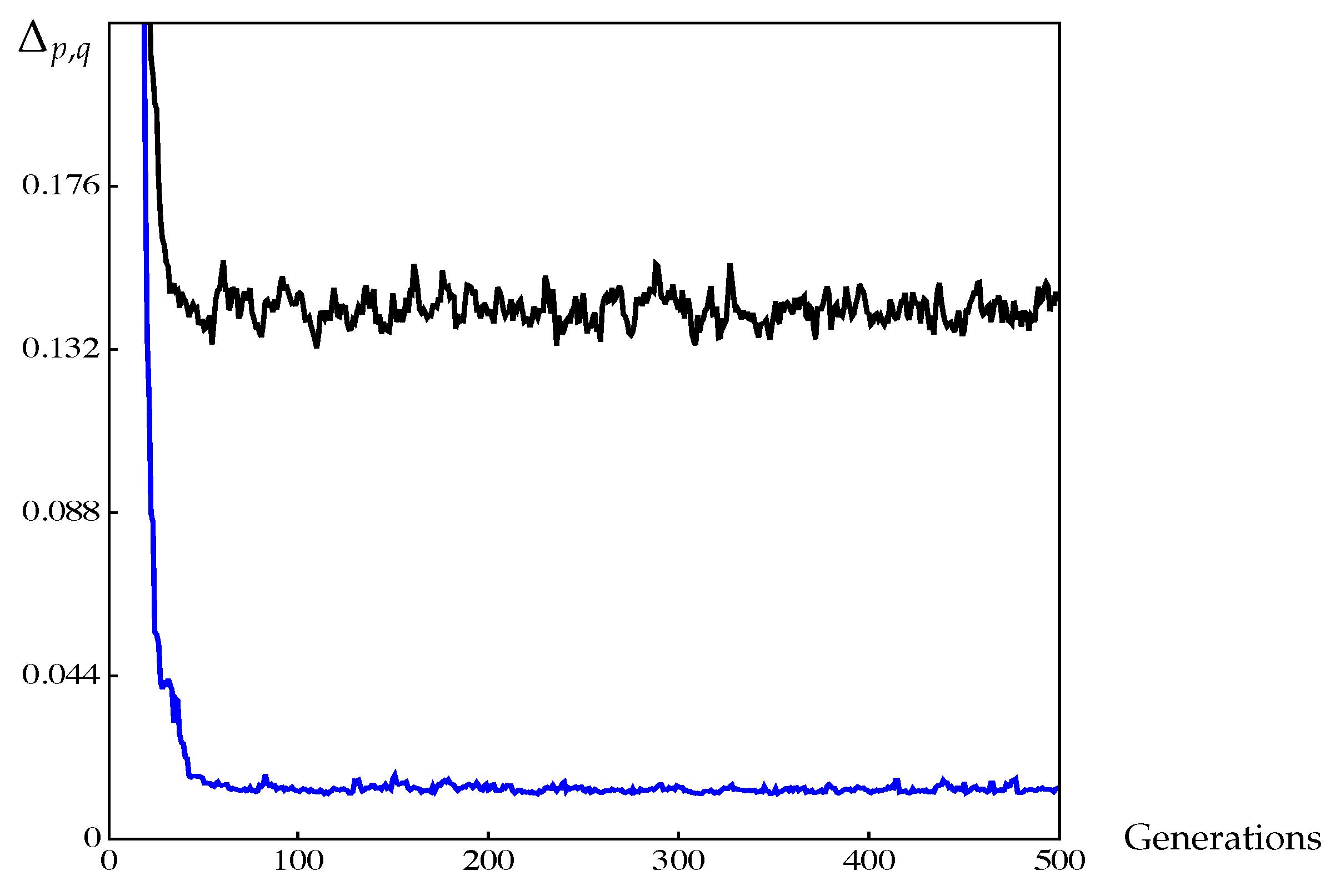
Figure 23.
The black curve is the value for the discrete approximation, and the blue one is the respective curve for the continuous approximation of NSGA-II for MOP (Equation (17)).
Figure 23.
The black curve is the value for the discrete approximation, and the blue one is the respective curve for the continuous approximation of NSGA-II for MOP (Equation (17)).
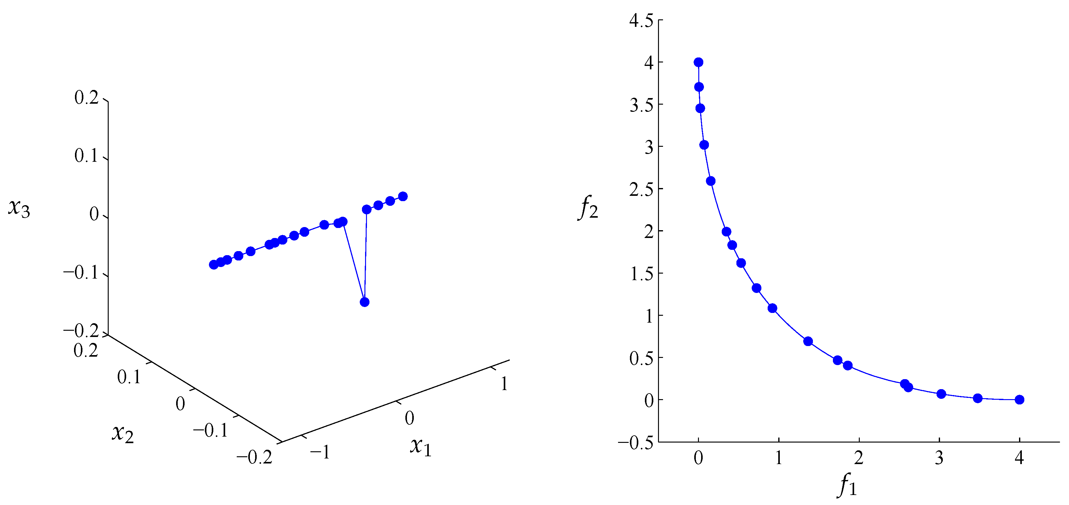
Figure 24.
(Left) The blue dots and the blue polygon line are the discrete and continuous approximation, respectively, for the Pareto set of MOP (Equation (17)) in the 300th generation. (Right) respective sets and of the Pareto front.
Figure 24.
(Left) The blue dots and the blue polygon line are the discrete and continuous approximation, respectively, for the Pareto set of MOP (Equation (17)) in the 300th generation. (Right) respective sets and of the Pareto front.
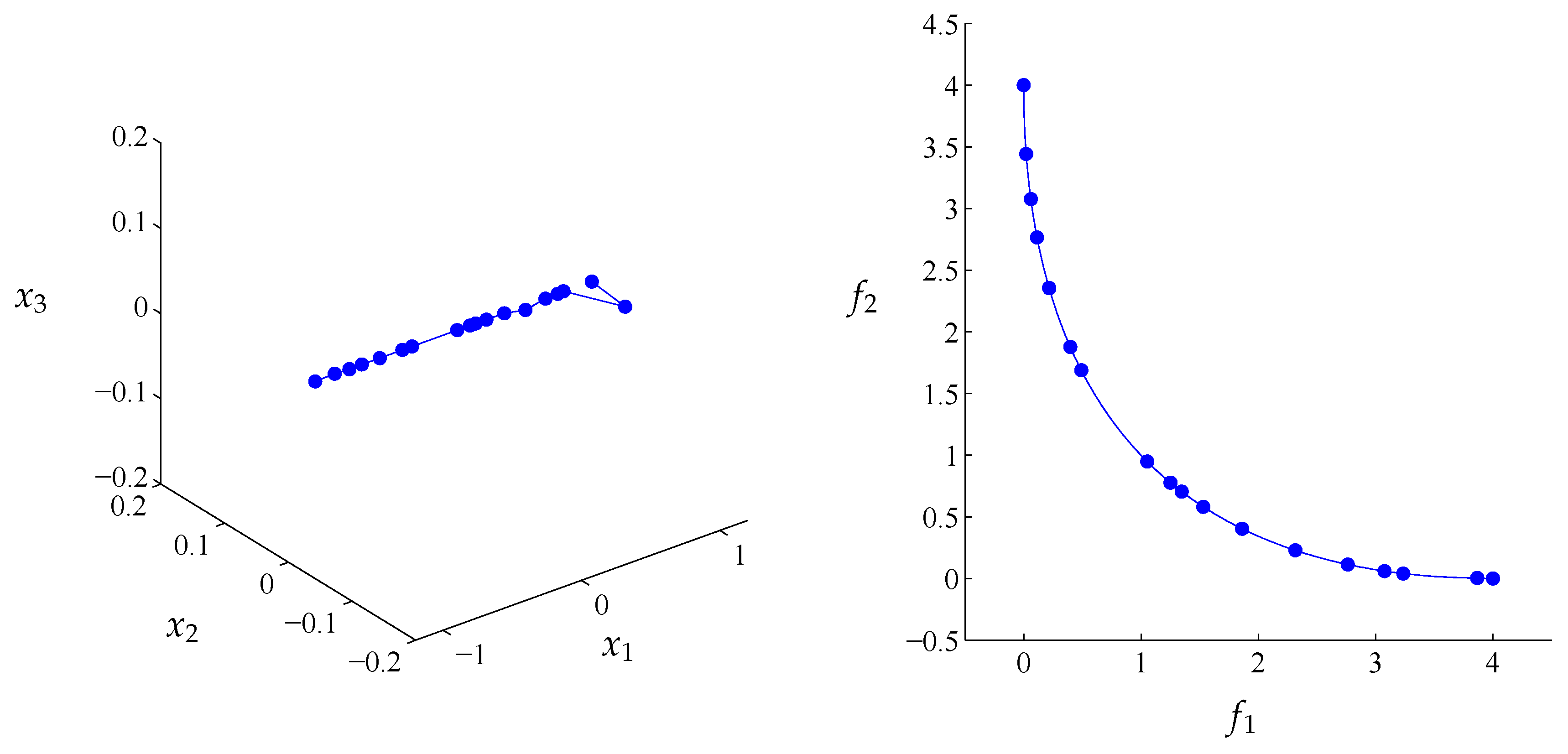
Figure 25.
The same as in
Figure 24 but for the 400th generation.
Figure 25.
The same as in
Figure 24 but for the 400th generation.
Figure 26.
The same as in
Figure 24 but for the 500th generation.
Figure 26.
The same as in
Figure 24 but for the 500th generation.
Table 1.
for several values of p and q.
Table 1.
for several values of p and q.
| | p | 1 | 2 | 5 | 10 | 20 |
|---|
| q | |
|---|
| | | | | |
| | | | | |
| | | | | |
| | | | | |
| | | | | |
| 1 | | | | | |
| 2 | | | | | |
| 5 | | | | | |
| 10 | | | | | |
Table 2.
for several values of p and q.
Table 2.
for several values of p and q.
| | p | 1 | 2 | 5 | 10 | 20 |
|---|
| q | |
|---|
| | | | | |
| | | | | |
| | | | | |
| | | | | |
| | | | | |
| 1 | | | | | |
| 2 | | | | | |
| 5 | | | | | |
| 10 | | | | | |
Table 3.
Triangle inequality violations, in percentage, for several values of p and q: Here, we randomly chose 80 sets, each one containing 2 points in , and verified the triangle inequality for all possible set permutations (that is, 492,960).
Table 3.
Triangle inequality violations, in percentage, for several values of p and q: Here, we randomly chose 80 sets, each one containing 2 points in , and verified the triangle inequality for all possible set permutations (that is, 492,960).
| | p | 1 | 2 | 5 | 10 |
|---|
| q | |
|---|
| | 0 | 0 | 0 |
| | | 0 | 0 |
| | | 0 | 0 |
| | | | 0 |
| | | | |
Table 4.
results between the sets A and in Equations (14) and (15) for and some parameter values of p, q, and .
Table 4.
results between the sets A and in Equations (14) and (15) for and some parameter values of p, q, and .
| p | q | | | | |
|---|
| 1 | 1 | | | | |
| 1 | 1 | | | | |
| 1 | 100 | | | | |
| 1 | 200 | | | | |
| 1 | | | | | |
Table 5.
results for the approximations of the Pareto set and front for MOP (Equation (16)).
Table 5.
results for the approximations of the Pareto set and front for MOP (Equation (16)).
| | p | q | Decision Space | Objective Space |
|---|
| | Finite Arch. | Cont. Arch. | Finite Arch. | Cont. Arch. |
|---|
| 1 | 1 | | | | |
| 1 | 1 | | | | |
| 1 | 100 | | | | |
| 1 | 200 | | | | |
| 1 | 10,000 | | | | |
| 1 | 1 | | | | |
| 1 | 1 | | | | |
| 1 | 100 | | | | |
| 1 | 200 | | | | |
| 1 | 10,000 | | | | |
Table 6.
Parameter setting for NSGA-II and MOEA/D: Here, n denotes the dimension of the decision variable space.
Table 6.
Parameter setting for NSGA-II and MOEA/D: Here, n denotes the dimension of the decision variable space.
| Algorithm | Parameter | Value |
|---|
| NSGA-II | Population size | 12 |
| Number of generations | 500 |
| Crossover probability | 0.8 |
| Mutation probability | |
| Distribution index for crossover | 20 |
| Distribution index for mutation | 20 |
| MOEA/D | Population size | 12 |
| # weight vectors | 12 |
| Number of generations | 500 |
| Crossover probability | 1 |
| Mutation probability | |
| Distribution index for crossover | 30 |
| Distribution index for mutation | 20 |
| Aggregation function | Tchebycheff |
| Neighborhood size | 3 |
Table 7.
For MOP (Equation (16)), the Table shows the results for the finite and continuous Pareto front approximations. We used the NSGA-II generated archives for and .
Table 7.
For MOP (Equation (16)), the Table shows the results for the finite and continuous Pareto front approximations. We used the NSGA-II generated archives for and .
| Generation | | |
|---|
| Finite Arch. | Cont. Arch. | Finite Arch. | Cont. Arch. |
|---|
| 50 | | | | |
| 100 | | | | |
| 200 | | | | |
| 250 | | | | |
| 400 | | | | |
| 450 | | | | |
| 460 | | | | |
| 470 | | | | |
| 480 | | | | |
| 490 | | | | |
| 500 | | | | |
Table 8.
For MOP (Equation (16)), the Table shows the results for the finite and continuous Pareto front approximations. We used the MOEA/D generated archives for and .
Table 8.
For MOP (Equation (16)), the Table shows the results for the finite and continuous Pareto front approximations. We used the MOEA/D generated archives for and .
| Generation | | |
|---|
| Finite Arch. | Cont. Arch. | Finite Arch. | Cont. Arch. |
|---|
| 50 | | | | |
| 100 | | | | |
| 200 | | | | |
| 250 | | | | |
| 400 | | | | |
| 450 | | | | |
| 460 | | | | |
| 470 | | | | |
| 480 | | | | |
| 490 | | | | |
| 500 | | | | |
Table 9.
results between the Pareto Front and its respective discrete and continuous approximations of NSGA-II for MOP (Equation (17)): The data shown is the averaged over the 20 independent runs above.
Table 9.
results between the Pareto Front and its respective discrete and continuous approximations of NSGA-II for MOP (Equation (17)): The data shown is the averaged over the 20 independent runs above.
| Generation | Continuous Archive | Finite Archive |
|---|
| 20 | | |
| 40 | | |
| 60 | | |
| 80 | | |
| 100 | | |
| 120 | | |
| 140 | | |
| 160 | | |
| 180 | | |
| 200 | | |
| 220 | | |
| 240 | | |
| 260 | | |
| 280 | | |
| 300 | | |
| 320 | | |
| 340 | | |
| 360 | | |
| 380 | | |
| 400 | | |
| 420 | | |
| 440 | | |
| 460 | | |
| 480 | | |
| 500 | | |
