Article

A Note on a Generalized Gerber–Shiu Discounted Penalty Function for a Compound Poisson Risk Model

1
Department of Humanities and Social Sciences, Yibin Vocational & Technical College, Yibin 644003, China
2
School of Insurance, Shandong University of Finance and Economics, Jinan 250014, China
3
School of Science, Shandong Jiaotong University, Jinan 250357, China
*
Author to whom correspondence should be addressed.
Mathematics 2019, 7(10), 891; https://doi.org/10.3390/math7100891
Submission received: 13 August 2019 / Revised: 19 September 2019 / Accepted: 20 September 2019 / Published: 24 September 2019
(This article belongs to the Special Issue Stochastic Processes: Theory and Applications)

Abstract

:
In this paper, we propose a new generalized Gerber–Shiu discounted penalty function for a compound Poisson risk model, which can be used to study the moments of the ruin time. First, by taking derivatives with respect to the original Gerber–Shiu discounted penalty function, we construct a relation between the original Gerber–Shiu discounted penalty function and our new generalized Gerber–Shiu discounted penalty function. Next, we use Laplace transform to derive a defective renewal equation for the generalized Gerber–Shiu discounted penalty function, and give a recursive method for solving the equation. Finally, when the claim amounts obey the exponential distribution, we give some explicit expressions for the generalized Gerber–Shiu discounted penalty function. Numerical illustrations are also given to study the effect of the parameters on the generalized Gerber–Shiu discounted penalty function.

1. Introduction

The classical compound Poisson risk process { U ( t ) } t 0 is defined by
U ( t ) = u + c t i = 1 N ( t ) X i , t 0 ,
where u is the non-negative amount of initial reserves, and c > 0 denotes the constant premium rate per unit time. The counting process { N ( t ) } t 0 , representing the total claim numbers up to time t, is a homogeneous Poisson processes with intensity λ . { X i } i 1 is a sequence of independent and identically distributed non-negative random variables, where X i is the i-th claim amount. Let f ( x ) denote the density function of X, and let E [ X ] and f ^ ( s ) = 0 e s x f ( x ) d x denote the expectation and Laplace transform of X, respectively. To avoid ruin from being a certain event, we assume c > λ E [ X ] .
We say that ruin occurs whenever U ( t ) becomes negative. The time to ruin of the insurance company is defined as
τ = inf { t : U ( t ) < 0 } ,
where τ = if for all t 0 , U ( t ) 0 . For the initial reserves U ( 0 ) = u , the probability of ruin is defined as
ψ ( u ) = P ( τ < | U ( 0 ) = u ) , u 0 .
The probability of ruin is an important risk measure in the study of ruin in risk theory. It has been widely studied in actuarial science. In 1998, famous actuarial scholars Hans Gerber and Elias Shiu first proposed an expected discounted penalty function, which is also called Gerber–Shiu discounted penalty function, to study ruin related problems. Recently, it has become a powerful risk measurement tool in ruin theory. Given the initial surplus U ( 0 ) = u , we define the classical Gerber–Shiu discounted penalty function as follows:
Φ ( u , δ ) = E [ e δ τ W ( U ( τ ) , | U ( τ ) | ) I ( τ < ) | U ( 0 ) = u ] , u 0 ,
where δ 0 is the force of interest, W ( x , y ) is a non-negative measurable penalty function, and I ( · ) is the indicator function. It is clear that the Gerber–Shiu discounted penalty function becomes the probability of ruin when δ = 0 , W ( x , y ) = 1 . For the recent literature on the Gerber–Shiu discounted penalty function, we can refer to work by Lin et al. [1], Zhang et al. [2], Yu [3,4], Wang et al. [5], Avram et al. [6], Zhang [7], Chi [8], Peng and Wang [9], Li et al. [10], Huang et al. [11], Preischl and Thonhauser [12], Zeng et al. [13,14], Yu et al. [15], Dickson and Qazvini [16], Zhang and Su [17,18], Li et al. [19], and Zhao and Yin [20], among others.
In recent years, Gerber–Shiu discounted penalty function has been extended by many actuarial scholars, so that the new risk measures can be used to study more related quantities. For example, Cai et al. [21] studied the ruin-related Gerber–Shiu discounted penalty risk measures by bringing in the conception of path consumption. Cheung [22] extended the Gerber–Shiu discounted penalty function by introducing the penultimate claim before ruin under a Sparre–Andersen renewal risk model. Chueng [23], Cheung and Woo [24] proposed a new Gerber–Shiu type function by incorporating the total claims up to ruin. Chueng and Feng [25] studied a new kind of generalized Gerber–Shiu discounted penalty function under the Markov arrival process. Wang and Li [26] extended the discount rate from constant to a random variable for the Gerber–Shiu discounted penalty function in the classical risk model. Wang and Zhang [27] provided a smooth extension of the Gerber–Shiu discounted penalty function by introducing an auxiliary function. As is known to all, the ruin time is also an important random variable in the study of risk theory. We can study the Laplace transform of the ruin time by the Gerber–Shiu discounted penalty function, while other mathematical characteristics associated with the ruin time cannot be directly studied through Gerber–Shiu discounted penalty function. In recent years, many actuarial scholars have paid attention to the moment of the ruin time. For instance, Egidio dos Reis [28], Lin and Willmot [29] and Drekic and Willmot [30] studied the moment of the ruin time under the compound Poisson risk model. Pitts and Politis [31] proposed an approximation approach of the moment of ruin time. Yu et al. [32] studied the moment of ruin time under the Markov arrival risk model. The moment of ruin time was introduced in the Gerber–Shiu discounted penalty function by Lee and Willmot [33]; then, they studied this new Gerber–Shiu discounted penalty function Sparre-Andersen risk model [34]. Schmidli [35] considered a new Gerber–Shiu discounted penalty function, which is modified with an additional penalty for reaching a level above the initial capital. Deng et al. [36] studied a generalized Gerber–Shiu discounted penalty function, in which the interest rates follow a Markov chain with finite state space. Li and Lu [37] studied the generalized expected discounted penalty function in a risk process with credit and debit interests.
In this paper, we introduce a new generalized Gerber–Shiu type function. For non-negative integer n, define
Φ n ( u , δ ) = E [ τ n e δ τ W ( U ( τ ) , | U ( τ ) | ) I ( τ < ) | U ( 0 ) = u ] , u 0 .
We call Φ n ( u , δ ) a generalized Gerber–Shiu discounted penalty function. It is obvious that Φ 0 ( u , δ ) = Φ ( u , δ ) . When W ( x , y ) = 1 , Φ n ( u , δ ) is the discounted nth moment of ruin time, then we can use it to study the expectation and variance of ruin time. Note that the generalized Gerber–Shiu discounted penalty function defined by formula (5) is different from the function studied in Lee and Willmot [34] since we bring in the surplus before ruin.
In this paper, we mainly discuss the calculation method of the generalized Gerber–Shiu discounted penalty function Φ n ( u , δ ) . In Section 2, we propose a recursion method by Laplace transform to calculate Φ n ( u , δ ) . In Section 3, we present an exact expression of Φ n ( u , δ ) when claim amounts are exponentially distributed. Numerical examples are also given to explain the effect of the related parameters. Finally, conclusions are given in Section 4.

2. Recursion Calculation of Φ n ( u , δ )

First, we define the Laplace transform of Φ n ( u , δ ) by
Φ ^ n ( u , δ ) = 0 e s u Φ n ( u , δ ) d u , R e ( s ) 0 .
For convenience, we introduce the Dickson–Hipp operator T s , which, for any integral function h on ( 0 , + ) , is defined as
T s h ( x ) = x e s ( y x ) h ( y ) d y = 0 e s y h ( x + y ) d y , x 0 .
It is easily seen that T s h ( 0 ) = 0 e s y h ( y ) d y = h ^ ( s ) . The Dickson–Hipp operator has interchangeability, that is to say, for s r ,
T s T r h ( x ) = T r T s h ( x ) = T s h ( x ) T r h ( x ) r s .
For for more properties of the Dickson–Hipp operator, we refer interested readers to Dickson and Hipp [38] and Li and Garrido [39].
When n = 0 , it follows from Gerber and Shiu [35] and Laplace transform that Φ ^ 0 ( s , δ ) satisfies the following equation:
{ c s λ ( 1 f ^ ( s ) ) δ } Φ ^ 0 ( s , δ ) = λ { ω ^ ( ρ ( δ ) ) ω ^ ( s ) } ,
where
ω ( u ) = u W ( u , x u ) f ( x ) d x ,
ω ^ ( s ) = 0 e s u ω ( u ) d u ,
and ρ ( δ ) is the positive root of the following equation
c s λ ( 1 f ^ ( s ) ) δ = 0 .
By Equation (6), we can obtain the renewal equation satisfied by Gerber–Shiu discounted penalty function Φ 0 ( u , δ ) , and we can further derive the analytic expression of Φ 0 ( u , δ ) . Now, we consider the case n 1 . The derivative of Φ n ( u , δ ) with respect to δ is given by
Φ n ( u , δ ) = ( 1 ) n d n d δ n Φ 0 ( u , δ ) .
Applying Laplace transform on both sides of Equation (8) gives
Φ ^ n ( s , δ ) = ( 1 ) n d n d δ n Φ ^ 0 ( s , δ ) .
Then, taking a derivative on both sides of Equation (6) with respect to δ yields
{ c s λ ( 1 f ^ ( s ) ) δ } d n d δ n Φ ^ 0 ( s , δ ) n d n 1 d δ n 1 Φ ^ 0 ( s , δ ) = λ d n d δ n ω ^ ( ρ ( δ ) ) .
In addition, by Equation(9), we have
{ c s λ ( 1 f ^ ( s ) ) δ } Φ ^ n ( s , δ ) + n Φ ^ n 1 ( s , δ ) = ( 1 ) n λ d n d δ n ω ^ ( ρ ( δ ) ) .
Setting s = ρ ( δ ) in Equation (10) yields
( 1 ) n λ d n d δ n ω ^ ( ρ ( δ ) ) = n Φ ^ n 1 ( ρ ( δ ) , δ ) .
Substituting the above result back into Equation (10) gives
{ c s λ ( 1 f ^ ( s ) ) δ } Φ ^ n ( s , δ ) = n Φ ^ n 1 ( ρ ( δ ) , δ ) n Φ ^ n 1 ( s , δ ) .
Since ρ ( δ ) is the root of Equation (7), we have
c s λ ( 1 f ^ ( s ) ) δ = c s λ ( 1 f ^ ( s ) ) δ { c ρ ( δ ) λ [ 1 f ^ ( ρ ( δ ) ) ] δ } = c ( s ρ ( δ ) ) + λ [ f ^ ( s ) f ^ ( ρ ( δ ) ) ] = ( s ρ ( δ ) ) c + λ f ^ ( s ) f ^ ( ρ ( δ ) ) s ρ ( δ ) = ( s ρ ( δ ) ) [ c λ T s T ρ ( δ ) f ( 0 ) ] .
Plugging Equation (12) back into Equation (11) gives
( s ρ ( δ ) ) [ c λ T s T ρ ( δ ) f ( 0 ) ] Φ ^ n ( s , δ ) = n Φ ^ n 1 ( ρ ( δ ) , δ ) n Φ ^ n 1 ( s , δ ) .
We can rewrite the above equation to obtain
1 λ c T s T ρ ( δ ) f ( 0 ) Φ ^ n ( s , δ ) = n c Φ ^ n 1 ( ρ ( δ ) , δ ) Φ ^ n 1 ( s , δ ) s ρ ( δ ) = n c T s T ρ ( δ ) Φ ^ n 1 ( 0 , δ ) .
Applying Laplace transform on both sides of Equation (13) gives
Φ n ( u , δ ) = 0 λ c T ρ ( δ ) f ( x ) Φ n ( u x , δ ) d x + n c T ρ ( δ ) Φ n 1 ( u , δ ) ,
where g ( x ) = λ c T ρ ( δ ) f ( x ) , x 0 . Since by Gerber and Shiu [40] we have 0 g ( x ) d x < 1 , then Equation (14) is a defective renewal equation.
Define
H ( u ) = n = 1 g n ( u ) , u 0 ,
where g n denotes the nth convolution of g. Then, we can express the solution of Equation (14) as follows:
Φ n ( u , δ ) = n c T ρ ( δ ) Φ n 1 ( u , δ ) + n c 0 u H ( u x ) T ρ ( δ ) Φ n 1 ( x , δ ) d x .
The above equation gives a recursion algorithm for computing Φ n ( u , δ ) , where the initial value is given by Φ 0 ( u , δ ) .

3. Explicit Expressions for Exponential Claim Distribution and Numerical Examples

In this section, we suppose that the claim amounts are exponentially distributed, and the density function is given by
f ( x ) = α e α x , α , x > 0 .
To obtain some explicit results, we assume the penalty function W ( x , y ) = W 1 ( y ) . Then, we have
ω ( u ) = u W 1 ( x u ) α e α x d x = β e α u ,
where β = 0 W 1 ( x ) α e α x d x . Solving Equation (7), we obtain
ρ ( δ ) = λ + δ c α + ( λ + δ c α ) 2 + 4 c α δ 2 c .
We denote the other root of Equation (7) by R ( δ ) ; then, it is easy to obtain
R ( δ ) = λ + δ c α ( λ + δ c α ) 2 + 4 c α δ 2 c .
Now, we derive an expression for Φ n ( u , δ ) by Laplace inverse transform. First, by Equation (6), we have
c s + α ( s ρ ( δ ) ) ( s + R ( δ ) ) Φ ^ 0 ( s , δ ) = λ β α + ρ ( δ ) λ β α + s .
Then, we obtain
Φ ^ 0 ( s , δ ) = λ β c ( α + ρ ( δ ) ) ( s + R ( δ ) ) .
Applying Laplace inverse transform in the above equation gives
Φ 0 ( u , δ ) = λ β c ( α + ρ ( δ ) ) e R ( δ ) u , u 0 .
Next, we consider n 1 . Combining the derivative of formula (19) w.r.t δ and Equation (8), we find that Φ n ( u , δ ) has the following expression:
Φ n ( u , δ ) = k = 0 n A n , k u k k ! e R ( δ ) u , u 0 .
Finally, we discuss how to determine the coefficients A n , k in formula (20).
When n = 0 , comparing Equations (19) and (20), we obtain
A 0 , 0 = λ β c [ α + ρ ( δ ) ] .
Taking the Laplace transform of formula (20) yields
Φ ^ n ( s , δ ) = k = 0 n A n , k [ s + R ( δ ) ] k + 1 .
By formulas (21) and (22), we have
Φ ^ n ( s , δ ) = n [ Φ ^ n 1 ( ρ ( δ ) , δ ) Φ ^ n 1 ( s , δ ) ] c s λ ( 1 f ^ ( s ) ) δ = n ( s + α ) c ( s ρ ( δ ) ) ( s + R ( δ ) ) k = 0 n 1 A n 1 , k · 1 ( ρ ( δ ) + R ( δ ) ) k + 1 1 ( s + R ( δ ) ) k + 1 = L n ( s ) [ s + R ( δ ) ] n + 1 ,
where
L n ( s ) = n ( s + α ) c ( s ρ ( δ ) ) k = 0 n 1 A n 1 , k · [ s + R ( δ ) ] n k 1 [ s + R ( δ ) ] k + 1 [ ρ ( δ ) + R ( δ ) ] k + 1 [ ρ ( δ ) + R ( δ ) ] k + 1
is an n-order polynomial.
By partial fraction expansion of formula (23), we obtain
A n , k = 1 ( n k ) ! d n k d s n k L n ( s ) | s = R ( δ ) , k = 0 , 1 , 2 , , n .
Noting that the polynomial L n ( s ) only depends on A n 1 , k , we can calculate A n , k recursively from A 0 , k .
Without losing generality, we give the explicit expressions of Φ n ( u , δ ) for n = 1 , 2 .
For n = 1 , from formula (20), we have
Φ 1 ( u , δ ) = A 1 , 0 · e R ( δ ) u + A 1 , 1 · u e R ( δ ) u , u 0 .
From formula (24), we have
L 1 ( s ) = A 0 , 0 · ( s + α ) c [ ρ ( δ ) + R ( δ ) ] .
By formulas (25) and (27), we have
A 1 , 0 = d d s L 1 ( s ) | s = R ( δ ) = A 0 , 0 c [ ρ ( δ ) + R ( δ ) ] , A 1 , 1 = L 1 ( R ( δ ) ) = A 0 , 0 · ( α R ( δ ) ) c [ ρ ( δ ) + R ( δ ) ] .
Then, by formula (26), we get
Φ 1 ( u , δ ) = A 0 , 0 c [ ρ ( δ ) + R ( δ ) ] e R ( δ ) u + A 0 , 0 · ( α R ( δ ) ) c [ ρ ( δ ) + R ( δ ) ] e R ( δ ) u , u 0 .
For n = 2 , from formula (20), we have
Φ 2 ( u , δ ) = A 2 , 0 · e R ( δ ) u + A 2 , 1 · u e R ( δ ) u + 1 2 A 2 , 2 · u 2 e R ( δ ) u , u 0 .
From formula (24), we have
L 2 ( s ) = 2 A 1 , 0 c [ ρ ( δ ) + R ( δ ) ] ( s + α ) ( s + R ( δ ) ) + 2 A 1 , 1 c [ ρ ( δ ) + R ( δ ) ] 2 ( s + α ) ( s + ρ ( δ ) + R ( δ ) ) ,
L 2 ( s ) = 2 A 1 , 0 · [ 2 s + R ( δ ) + α ] c [ ρ ( δ ) + R ( δ ) ] + 2 A 1 , 1 · [ 2 s + 2 R ( δ ) + α + ρ ( δ ) ] c [ ρ ( δ ) + R ( δ ) ] 2 ,
L 2 ( s ) = 4 A 1 , 0 c [ ρ ( δ ) + R ( δ ) ] + 4 A 1 , 1 c [ ρ ( δ ) + R ( δ ) ] 2 .
By formulas (25) and (30)–(32), we have
A 2 , 0 = 1 2 d 2 d s 2 L 2 ( s ) | s = R ( δ ) = 2 A 1 , 0 c [ ρ ( δ ) + R ( δ ) ] + 2 A 1 , 1 c [ ρ ( δ ) + R ( δ ) ] 2 , A 2 , 1 = d d s L 2 ( s ) | s = R ( δ ) = 2 A 1 , 0 · [ α R ( δ ) ] c [ ρ ( δ ) + R ( δ ) ] + 2 A 1 , 1 · [ α + ρ ( δ ) ] c [ ρ ( δ ) + R ( δ ) ] 2 , A 2 , 2 = L 2 ( s ) | s = R ( δ ) = 2 A 1 , 1 · [ α R ( δ ) ] c [ ρ ( δ ) + R ( δ ) ] .
Then, by formula (29), we get
Φ 2 ( u , δ ) = { 2 A 1 , 0 c [ ρ ( δ ) + R ( δ ) ] + 2 A 1 , 1 c [ ρ ( δ ) + R ( δ ) ] 2 } e R ( δ ) u + 2 A 1 , 0 · [ α R ( δ ) ] c [ ρ ( δ ) + R ( δ ) ] + 2 A 1 , 1 · [ α + ρ ( δ ) ] c [ ρ ( δ ) + R ( δ ) ] 2 u e R ( δ ) u + A 1 , 1 · [ α R ( δ ) ] c [ ρ ( δ ) + R ( δ ) ] u 2 e R ( δ ) u , u 0 .
Next, we give the numerical simulation of Φ 0 ( u , δ ) , Φ 1 ( u , δ ) and Φ 2 ( u , δ ) to illustrate the effect of the related parameters on the generalized Gerber–Shiu discounted penalty function by Matlab (Version: matlab2016a; Manufacturer: The MathWorks, Inc.; Natick, Massachusetts 01760 USA)
Example 1.
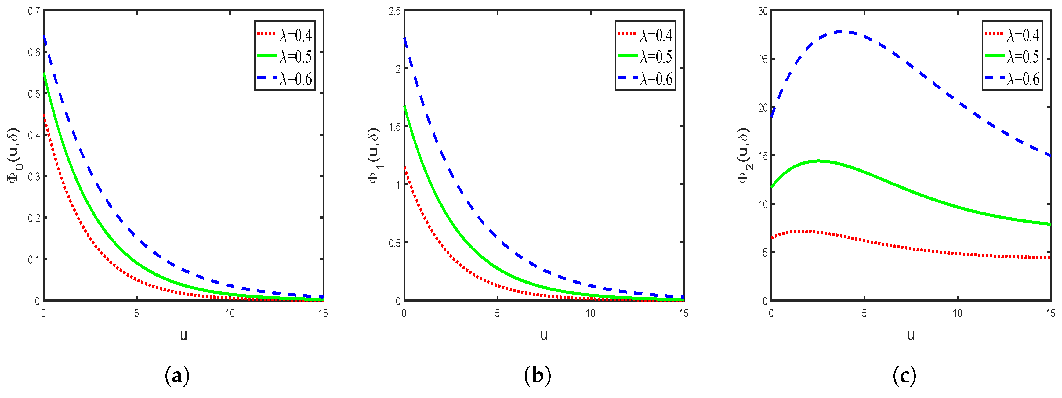
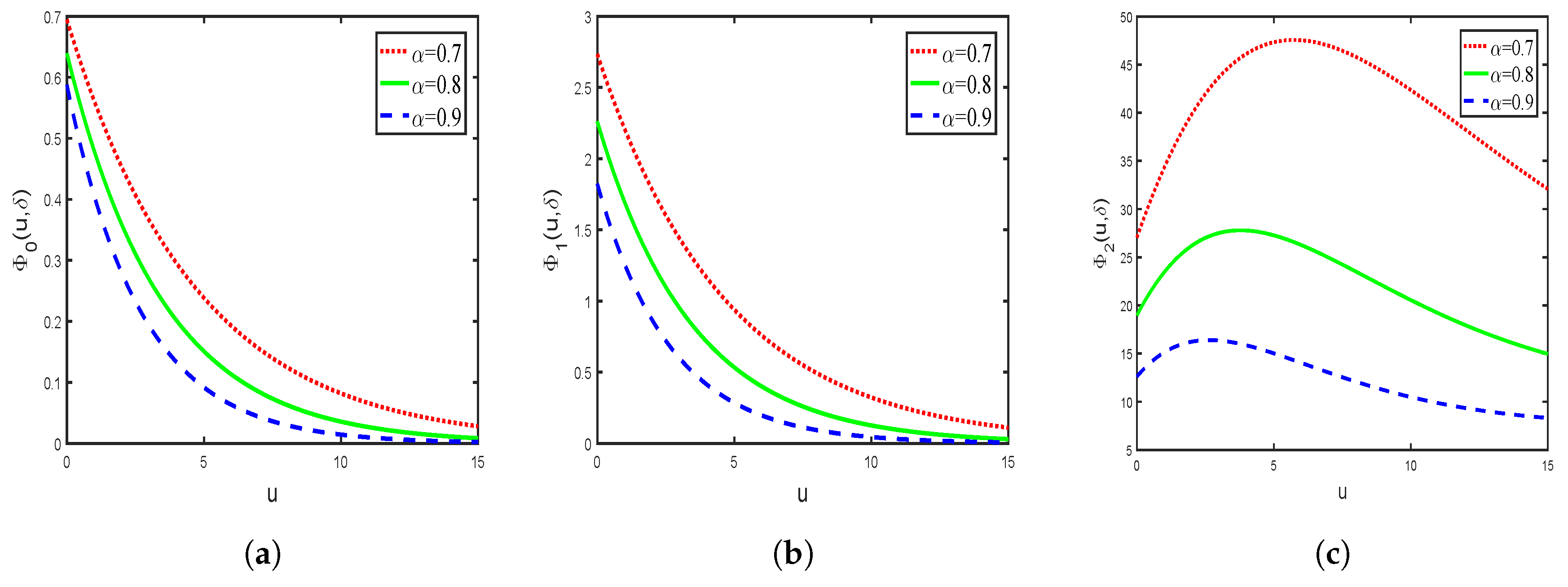
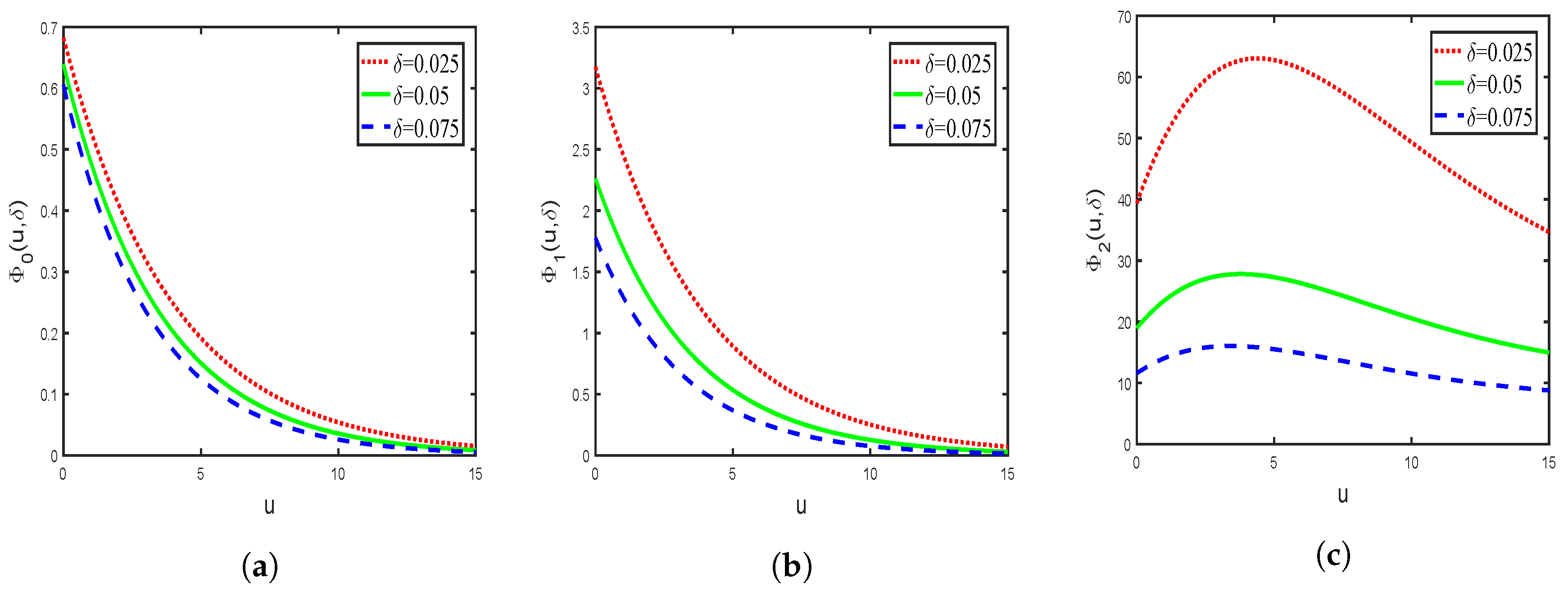
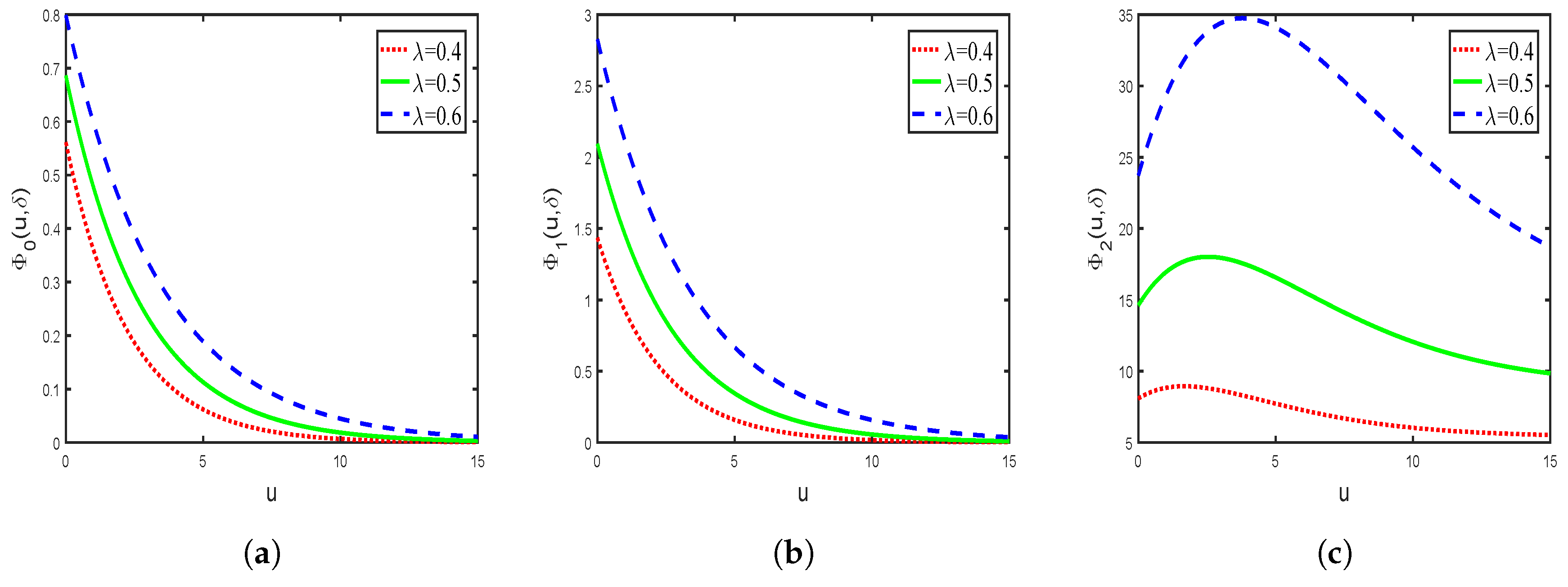
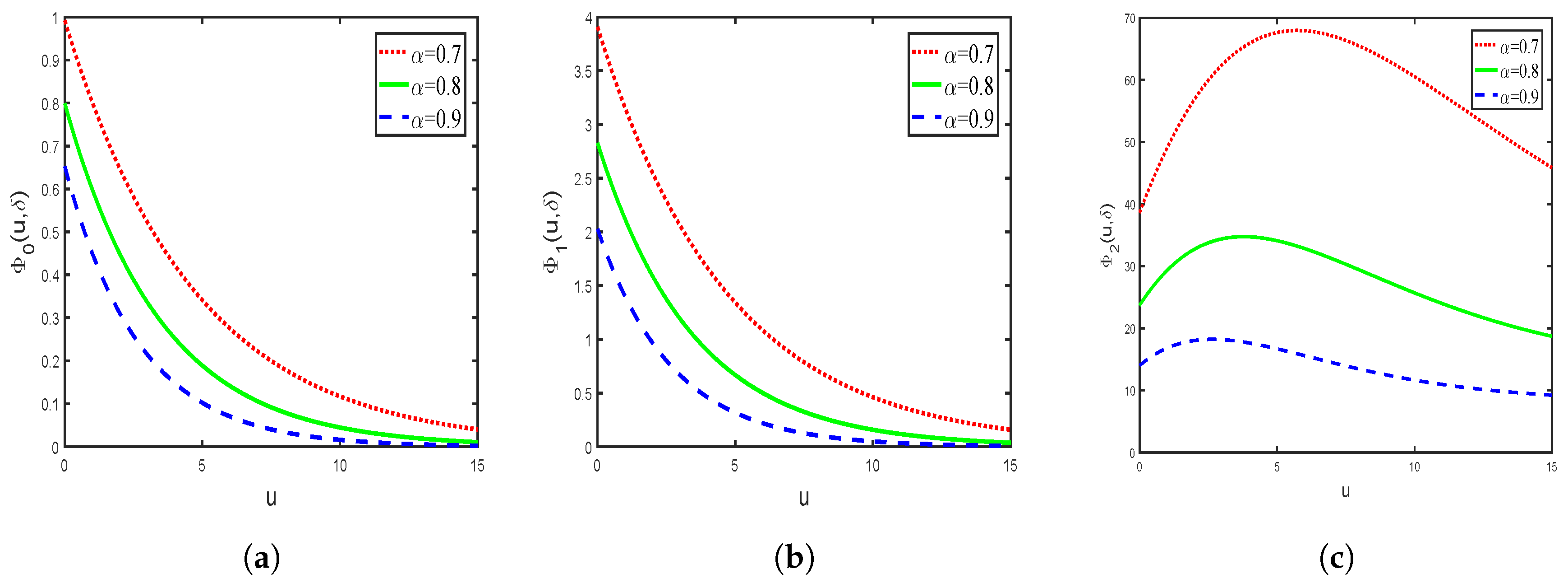
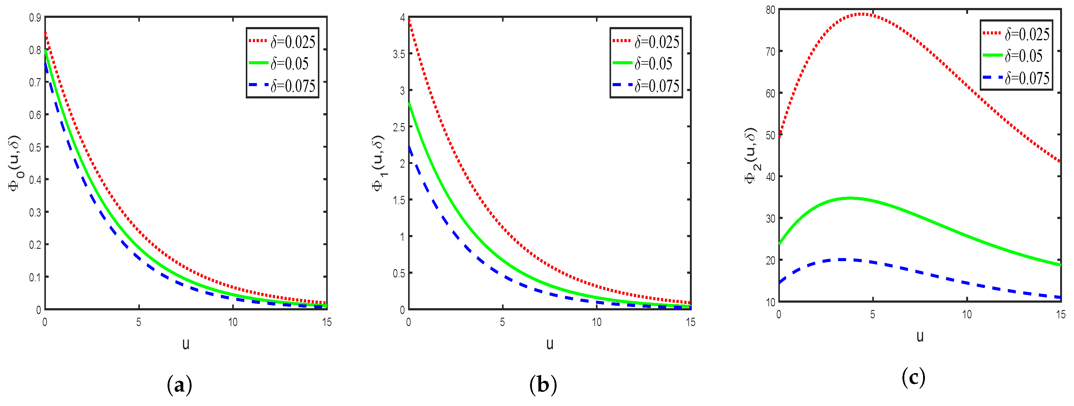
Suppose W ( x , y ) = 1 , then β = 1 . We give the influence of the relevant parameters on the function Φ 0 ( u , δ ) , Φ 1 ( u , δ ) and Φ 2 ( u , δ ) . See Figure 1, Figure 2, Figure 3 and Figure 4.
It is easy to see that the images we get from Figure 1, Figure 2, Figure 3 and Figure 4 are the opposite of the images some scholars get from the traditional classical risk model. For example, in Figure 1, Φ 0 ( u , δ ) is the Laplace transform of the ruin time. Φ 0 ( u , δ ) goes down as c increases. This means that the higher the premium income rate c is, the smaller the function Φ 0 ( u , δ ) is. The reason is that e δ τ is a decreasing function of τ . Increased premiums mean greater ruin time τ , which in turn leads to smaller functions e δ τ . Similarly, τ e δ τ and τ 2 e δ τ are also a subtractive function of τ when τ is large. Thus, Φ 1 ( u , δ ) and Φ 2 ( u , δ ) go down as c increases. The same conclusion appears in Figure 2, Figure 3 and Figure 4. We are not explain it one more time in the following Figure 5, Figure 6, Figure 7 and Figure 8.
Example 2.
Suppose W ( x , y ) = y , then β = 1 α . We give the influence of the relevant parameters on the function Φ 0 ( u , δ ) , Φ 1 ( u , δ ) and Φ 2 ( u , δ ) . See Figure 5, Figure 6, Figure 7 and Figure 8.

4. Conclusions

In this paper, we discuss a generalized Gerber–Shiu discounted penalty function, which relies on the moment of the time to ruin under the compound Poisson risk model. We present a recursion algorithm for calculating the generalized Gerber–Shiu discounted penalty function by Laplace transform and renewal theory when the claim amounts are subject to an exponential distribution. Furthermore, we derive some explicit expressions of the generalized Gerber–Shiu discounted penalty function for n = 0 , 1 , 2 . In addition, we also give numerical examples to explain the effects of parameters c , λ , α and δ on the generalized Gerber–Shiu discounted penalty function Φ 0 ( u , δ ) , Φ 1 ( u , δ ) and Φ 2 ( u , δ ) . It is very easy to see the effects of these parameters on the generalized Gerber–Shiu discounted penalty function from Figure 1, Figure 2, Figure 3, Figure 4, Figure 5, Figure 6, Figure 7 and Figure 8. The insurance company can bring the real claim data into the model for numerical simulation and obtain relevant parameters, so that the ruin probability, the Laplace transform of the ruin time and the discounted expected time to ruin can be calculated. The acquisition of these actuarial quantities will effectively improve the operating level of the insurance company.

Author Contributions

Data curation, W.Y., Y.S., Y.H. and X.Y.; Methodology, J.R. and W.Y.; Software, W.Y., K.S. and Y.S.; Writing—original draft, J.R. and W.Y.

Funding

This research is partially supported by the National Social Science Foundation of China (Grant No. 15BJY007), the National Natural Science Foundation of China (Grant Nos. 11301303, 71804090), the Taishan Scholars Program of Shandong Province (Grant No. tsqn20161041), the Humanities and Social Sciences Project of the Ministry Education of China (Grant No. 16YJC630070, Grant No. 19YJA910002), the Natural Science Foundation of Shandong Province (Grant No. ZR2018MG002), the Fostering Project of Dominant Discipline and Talent Team of Shandong Province Higher Education Institutions (Grant No. 1716009), the 1251 Talent Cultivation Project of Shandong Jiaotong University, the Risk Management and Insurance Research Team of Shandong University of Finance and Economics, the Shandong Jiaotong University ’Climbing’ Research Innovation Team Program, and the Collaborative Innovation Center Project of the Transformation of New and Old Kinetic Energy and Government Financial Allocation.

Acknowledgments

The authors would like to thank the four anonymous referees for their helpful comments and suggestions, which improved an earlier version of the paper.

Conflicts of Interest

The authors declare no conflict of interest.

References

  1. Lin, X.S.; Willmot, G.E.; Drekic, S. The classical risk model with a constant dividend barrier: Analysis of the Gerber–Shiu discounted penalty function. Insur. Math. Econ. 2003, 33, 391–408. [Google Scholar]
  2. Zhang, H.Y.; Zhou, M.; Guo, J.Y. The Gerber–Shiu discounted penalty function for classical risk model with a two-step premium rate. Stat. Probab. Lett. 2006, 76, 1211–1218. [Google Scholar] [CrossRef]
  3. Yu, W.G. Some results on absolute ruin in the perturbed insurance risk model with investment and debit interests. Econ. Model. 2013, 31, 625–634. [Google Scholar] [CrossRef]
  4. Yu, W.G. On the expected discounted penalty function for a Markov regime switching risk model with stochastic premium income. Discret. Dyn. Nat. Soc. 2013, 2013, 1–9. [Google Scholar] [CrossRef]
  5. Wang, Y.Y.; Yu, W.G.; Huang, Y.J.; Yu, X.L.; Fan, H.L. Estimating the expected discounted penalty function in a compound Poisson insurance risk model with mixed premium income. Mathematics 2019, 7, 305. [Google Scholar] [CrossRef]
  6. Avram, F.; Palmowski, Z.; Pistorius, M.R. On Gerber–Shiu functions and optimal dividend distribution for a Lévy risk process in the presence of a penalty function. Ann. Appl. Probab. 2015, 25, 1868–1935. [Google Scholar] [CrossRef]
  7. Zhang, Z.M. Estimating the Gerber–Shiu function by Fourier-Sinc series expansion. Scand. Actuar. J. 2017, 2017, 898–919. [Google Scholar] [CrossRef]
  8. Chi, Y.C. Analysis of expected discounted penalty function for a general jump diffusion risk model and applications in finance. Insur. Math. Econ. 2010, 46, 385–396. [Google Scholar] [CrossRef]
  9. Peng, J.Y.; Wang, D.C. Uniform asymptotics for ruin probabilities in a dependent renewal risk model with stochastic return on investments. Stochastics 2018, 90, 432–471. [Google Scholar] [CrossRef]
  10. Li, S.M.; Lu, Y.; Sendova, K.P. The expected discounted penalty function: From infinite time to finite time. Scand. Actuar. J. 2019, 2019, 336–354. [Google Scholar] [CrossRef]
  11. Huang, Y.J.; Yu, W.G.; Pan, Y.; Cui, C.R. Estimating the Gerber–Shiu expected discounted penalty function for Lévy risk model. Discrete Dyn. Nat. Soc. 2019, 2019, 1–15. [Google Scholar] [CrossRef]
  12. Preischl, M.; Thonhauser, S. Optimal reinsurance for Gerber–Shiu functions in the Cramér-Lundberg model. Insur. Math. Econ. 2019, 87, 82–91. [Google Scholar] [CrossRef]
  13. Zeng, Y.; Li, D.P.; Chen, Z.; Yang, Z. Ambiguity aversion and optimal derivative–based pension investment with stochastic income and volatility. J. Econ. Dyn. Control 2018, 88, 70–103. [Google Scholar] [CrossRef]
  14. Zeng, Y.; Li, D.P.; Gu, A.L. Robust equilibrium reinsurance–investment strategy for a mean–variance insurer in a model with jumps. Insur. Math. Econ. 2016, 66, 138–152. [Google Scholar] [CrossRef]
  15. Yu, W.G.; Huang, Y.J.; Cui, C.R. The absolute ruin insurance risk model with a threshold dividend strategy. Symmetry 2018, 10, 377. [Google Scholar] [CrossRef]
  16. Dickson, D.C.M.; Qazvini, M. Gerber–Shiu analysis of a risk model with capital injections. Eur. Actuar. J. 2016, 6, 409–440. [Google Scholar] [CrossRef]
  17. Zhang, Z.M.; Su, W. A new efficient method for estimating the Gerber–Shiu function in the classical risk model. Scand. Actuar. J. 2018, 2018, 426–449. [Google Scholar] [CrossRef]
  18. Zhang, Z.M.; Su, W. Estimating the Gerber–Shiu function in a Lévy risk model by Laguerre series expansion. J. Comput. Appl. Math. 2019, 346, 133–149. [Google Scholar] [CrossRef]
  19. Li, J.C.; Dickson, D.C.M.; Li, S.M. Some ruin problems for the MAP risk model. Insur. Math. Econ. 2015, 65, 1–8. [Google Scholar] [CrossRef]
  20. Zhao, Y.X.; Yin, C.C. The expected discounted penalty function under a renewal risk model with stochastic income. Appl. Math. Comput. 2012, 218, 6144–6154. [Google Scholar] [CrossRef]
  21. Cai, J.; Feng, R.; Willmot, G.E. On the total discounted operating costs up to default and its applications. Adv. Appl. Probab. 2009, 41, 495–522. [Google Scholar] [CrossRef]
  22. Cheung, E.C.K. A generalized penalty function in Sparre–Andersen risk models with surplus-dependent premium. Insur. Math. Econ. 2011, 48, 384–397. [Google Scholar] [CrossRef]
  23. Cheung, E.C.K. Moments of discounted aggregate claim costs until ruin in a Sparre–Andersen risk model with general interclaim times. Insur. Math. Econ. 2013, 53, 343–354. [Google Scholar] [CrossRef]
  24. Cheung, E.C.K.; Woo, J.K. On the discounted aggregate claim costs until ruin in dependent Sparre–Andersen risk processes. Scand. Actuar. J. 2016, 2016, 63–91. [Google Scholar] [CrossRef]
  25. Cheung, E.C.K.; Feng, R. A unified analysis of claim costs up to ruin in a Markovian arrival risk process. Insur. Math. Econ. 2013, 53, 98–109. [Google Scholar] [CrossRef]
  26. Wang, H.C.; Li, N.X. On the Gerber–Shiu function with random discount rate. Commun. Stat. Theory Methods 2017, 46, 210–220. [Google Scholar] [CrossRef]
  27. Wang, W.Y.; Zhang, Z.M. Computing the Gerber–Shiu function by frame duality projection. Scand. Actuar. J. 2019, 2019, 291–307. [Google Scholar] [CrossRef]
  28. Egidio dos Reis, A.D. On the moments of ruin and recovery times. Insur. Math. Econ. 2000, 27, 331–343. [Google Scholar] [CrossRef]
  29. Lin, X.S.; Willmot, G.E. The moments of the time of ruin, the surplus before ruin, and the deficit at ruin. Insur. Math. Econ. 2000, 27, 19–44. [Google Scholar] [CrossRef]
  30. Drekic, S.; Willmot, G.E. On the moments of the time of ruin with applications to phase-type claims. N. Am. Actuar. J. 2005, 9, 17–30. [Google Scholar] [CrossRef]
  31. Pitts, S.M.; Politis, K. Approximations for the moments of ruin time in the compound Poisson model. Insur. Math. Econ. 2008, 42, 668–679. [Google Scholar] [CrossRef]
  32. Yu, K.; Ren, J.; Stanford, D.A. The moments of the time of ruin in Markovian risk models. N. Am. Actuar. J. 2010, 14, 464–471. [Google Scholar] [CrossRef]
  33. Lee, W.Y.; Willmot, G.E. On the moments of the time to ruin in dependent Sparre–Andersen models with emphasis on Coxian interclaim times. Insur. Math. Econ. 2014, 59, 1–10. [Google Scholar] [CrossRef]
  34. Lee, W.Y.; Willmot, G.E. The moments of the time to ruin in dependent Sparre–Andersen models with Coxian claim sizes. Scand. Actuar. J. 2016, 2016, 550–564. [Google Scholar] [CrossRef]
  35. Schmidli, H. Extended Gerber–Shiu functions in a risk model with interest. Insur. Math. Econ. 2015, 61, 271–275. [Google Scholar] [CrossRef]
  36. Deng, Y.C.; Liu, J.; Huang, Y.; Li, M.; Zhou, J.M. On a discrete interaction risk model with delayed claims and stochastic incomes under random discount rates. Commun. Stat. Theory Methods 2018, 47, 5867–5883. [Google Scholar] [CrossRef]
  37. Li, S.M.; Lu, Y. On the generalized Gerber–Shiu function for surplus processes with interest. Insur. Math. Econ. 2013, 52, 127–134. [Google Scholar] [CrossRef]
  38. Dickson, D.C.M.; Hipp, C. On the time to ruin for Erlang (2) risk processes. Insur. Math. Econ. 2001, 29, 333–344. [Google Scholar] [CrossRef]
  39. Li, S.M.; Garrido, J. On ruin for the Erlang(n) risk process. Insur. Math. Econ. 2004, 34, 391–408. [Google Scholar] [CrossRef]
  40. Gerber, H.U.; Shiu, E.S.W. On the time value of ruin. N. Am. Actuar. J. 1998, 2, 48–72. [Google Scholar] [CrossRef]
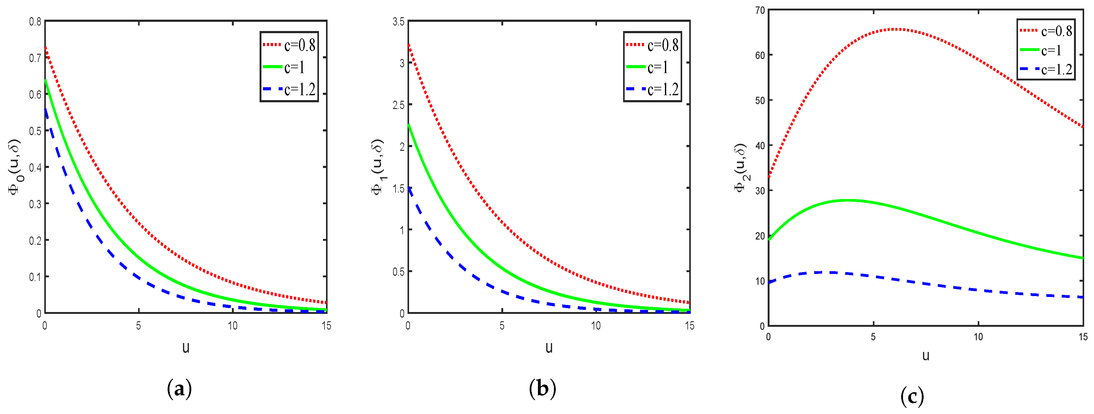
Figure 1. Set λ = 0.6 , α = 0.8 , δ = 0.05 . (a) The influence of the parameter c on the function Φ 0 ( u , δ ) . (b) The influence of the parameter c on the function Φ 1 ( u , δ ) . (c) The influence of the parameter c on the function Φ 2 ( u , δ ) .
Mathematics 07 00891 g001
Figure 2. Set c = 1 , α = 0.8 , δ = 0.05 . (a) The influence of the parameter λ on the function Φ 0 ( u , δ ) . (b) The influence of the parameter λ on the function Φ 1 ( u , δ ) . (c) The influence of the parameter λ on the function Φ 2 ( u , δ ) .
Mathematics 07 00891 g002
Figure 3. Set c = 1 , λ = 0.6 , δ = 0.05 . (a) The influence of the parameter α on the function Φ 0 ( u , δ ) . (b) The influence of the parameter α on the function Φ 1 ( u , δ ) . (c) The influence of the parameter α on the function Φ 2 ( u , δ ) .
Mathematics 07 00891 g003
Figure 4. Set c = 1 , λ = 0.6 , α = 0.8 . (a) The influence of the parameter δ on the function Φ 0 ( u , δ ) . (b) The influence of the parameter δ on the function Φ 1 ( u , δ ) . (c) The influence of the parameter δ on the function Φ 2 ( u , δ ) .
Mathematics 07 00891 g004
Figure 5. Set λ = 0.6 , α = 0.8 , δ = 0.05 . (a) The influence of the parameter c on the function Φ 0 ( u , δ ) . (b) The influence of the parameter c on the function Φ 1 ( u , δ ) . (c) The influence of the parameter c on the function Φ 2 ( u , δ ) .
Mathematics 07 00891 g005
Figure 6. Set c = 1 , α = 0.8 , δ = 0.05 . (a) The influence of the parameter λ on the function Φ 0 ( u , δ ) . (b) The influence of the parameter λ on the function Φ 1 ( u , δ ) . (c) The influence of the parameter λ on the function Φ 2 ( u , δ ) .
Mathematics 07 00891 g006
Figure 7. Set c = 1 , λ = 0.6 , δ = 0.05 . (a) The influence of the parameter α on the function Φ 0 ( u , δ ) . (b) The influence of the parameter α on the function Φ 1 ( u , δ ) . (c) The influence of the parameter α on the function Φ 2 ( u , δ ) .
Mathematics 07 00891 g007
Figure 8. Set c = 1 , λ = 0.6 , α = 0.8 . (a) The influence of the parameter δ on the function Φ 0 ( u , δ ) . (b) The influence of the parameter δ on the function Φ 1 ( u , δ ) . (c) The influence of the parameter δ on the function Φ 2 ( u , δ ) .
Mathematics 07 00891 g008