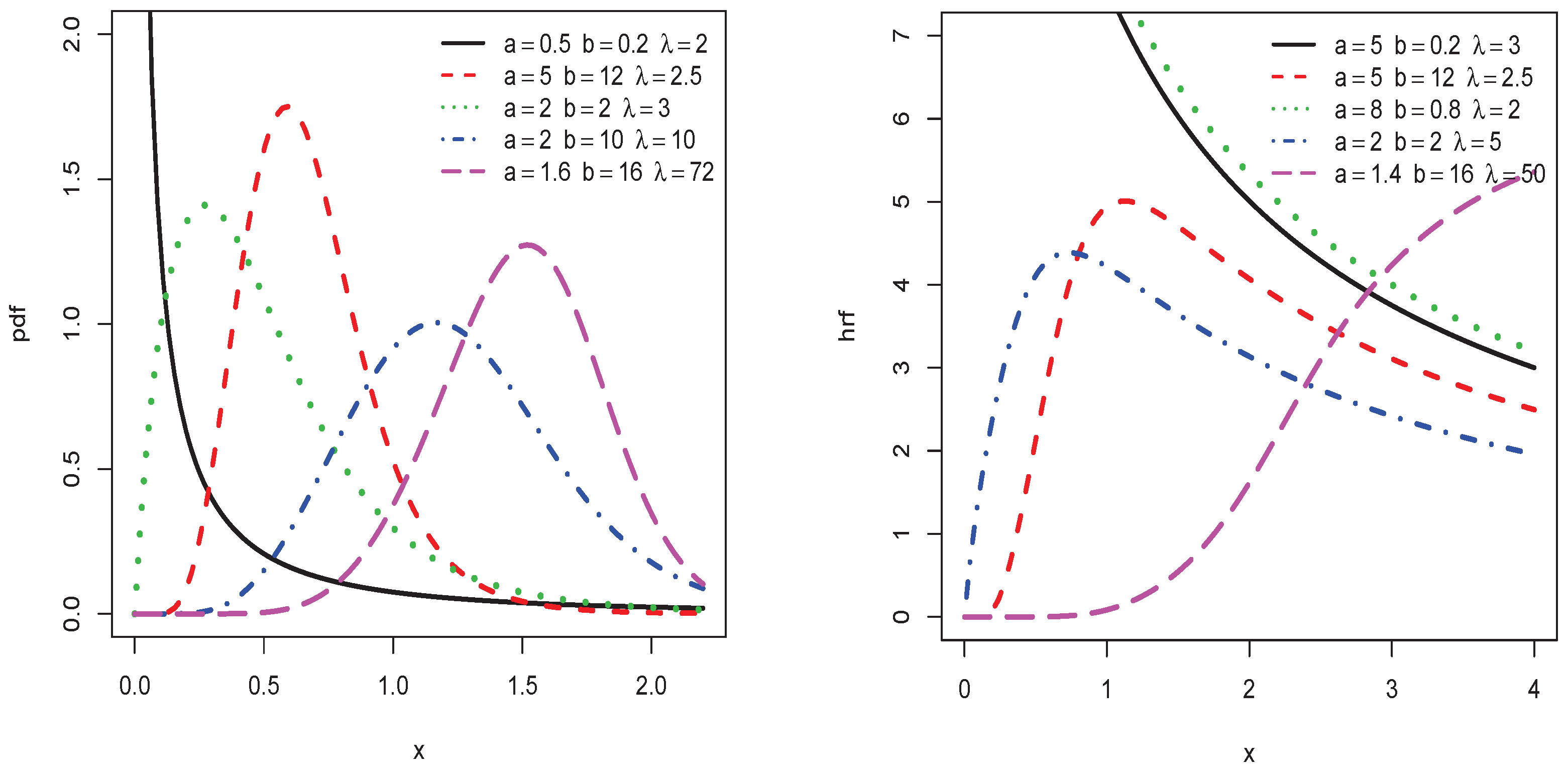
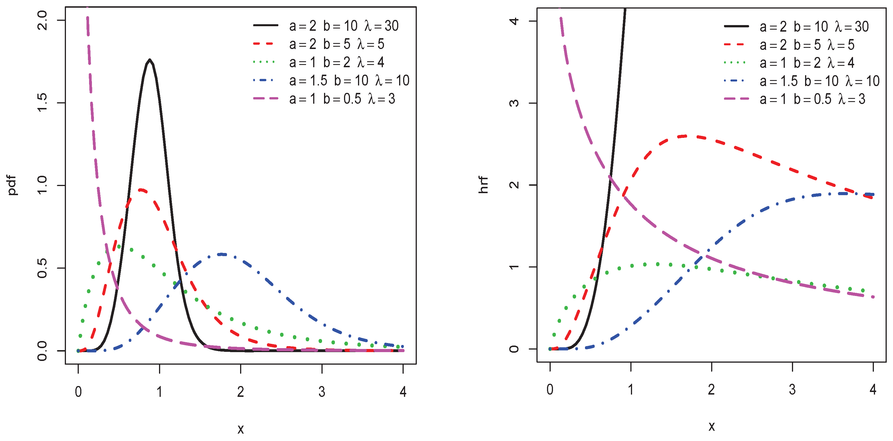
Figure 1.
Plots of some probability density functions (pdfs) and hazard rate functions (hrfs) of the type I half-logistic inverted Kumaraswamy (TIHLIK) distribution.
Figure 1.
Plots of some probability density functions (pdfs) and hazard rate functions (hrfs) of the type I half-logistic inverted Kumaraswamy (TIHLIK) distribution.
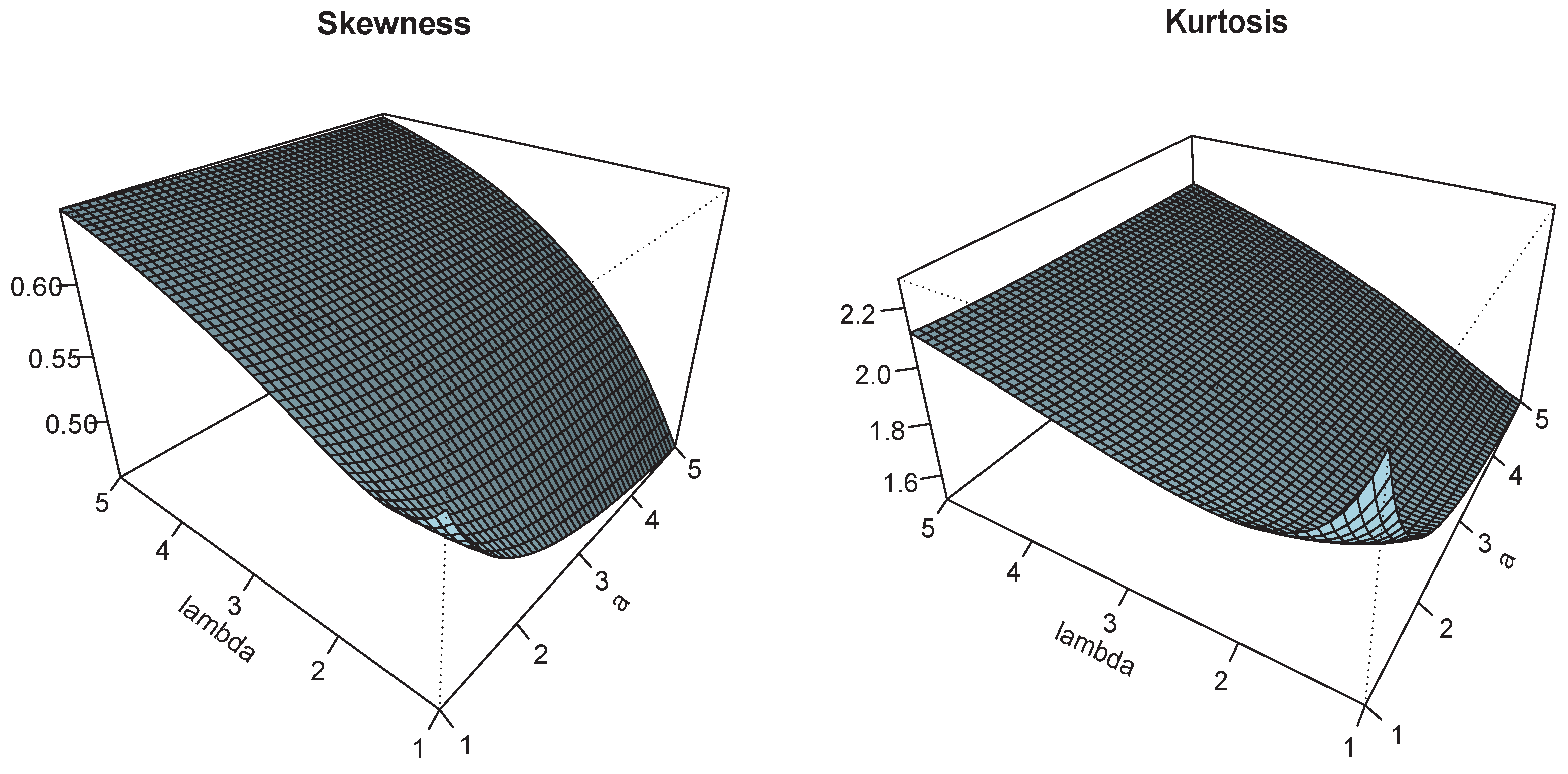
Figure 2.
Plots of some pdfs and hrfs of the TIHLIK distribution.
Figure 2.
Plots of some pdfs and hrfs of the TIHLIK distribution.
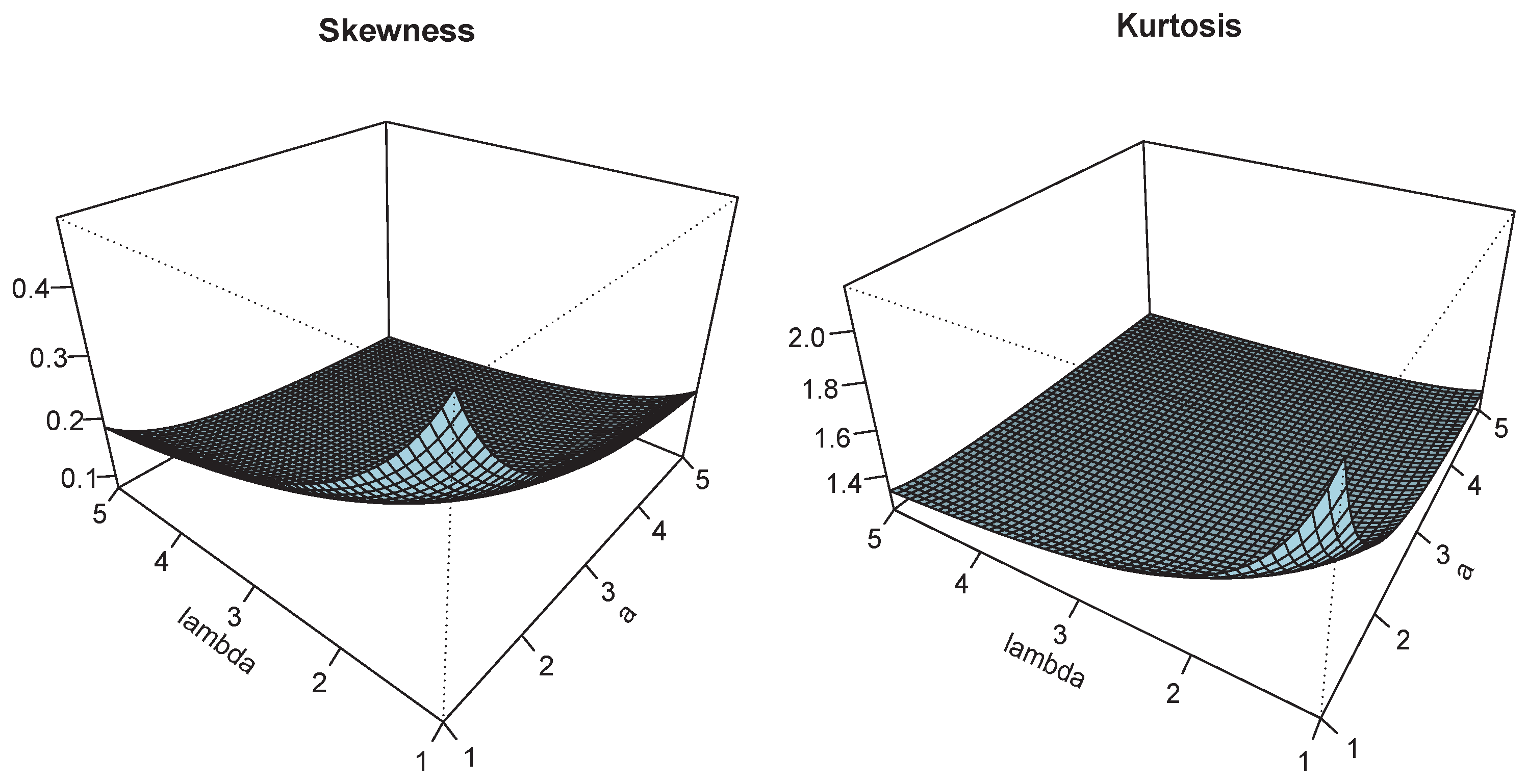
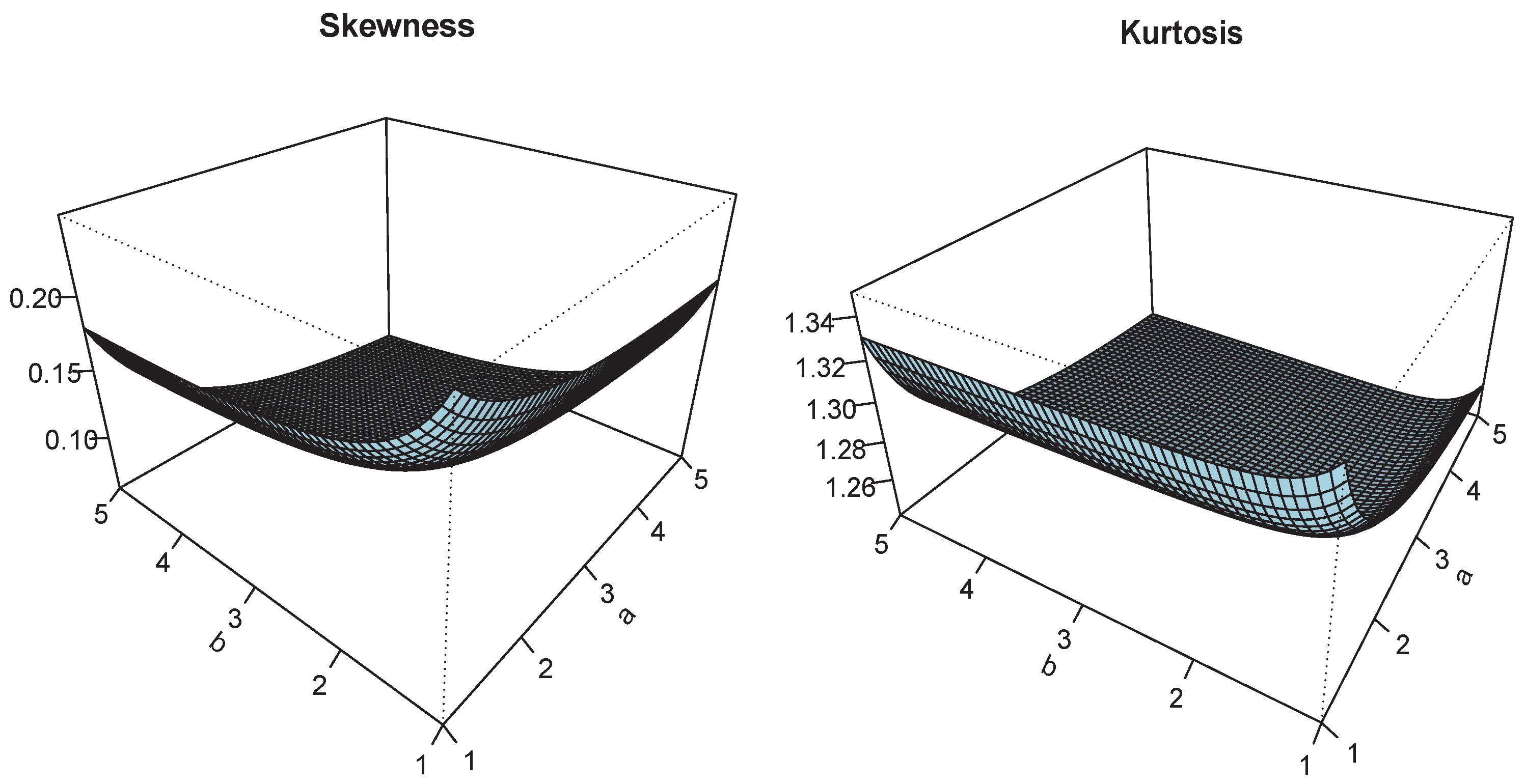
Figure 3.
Plots of and for and .
Figure 3.
Plots of and for and .
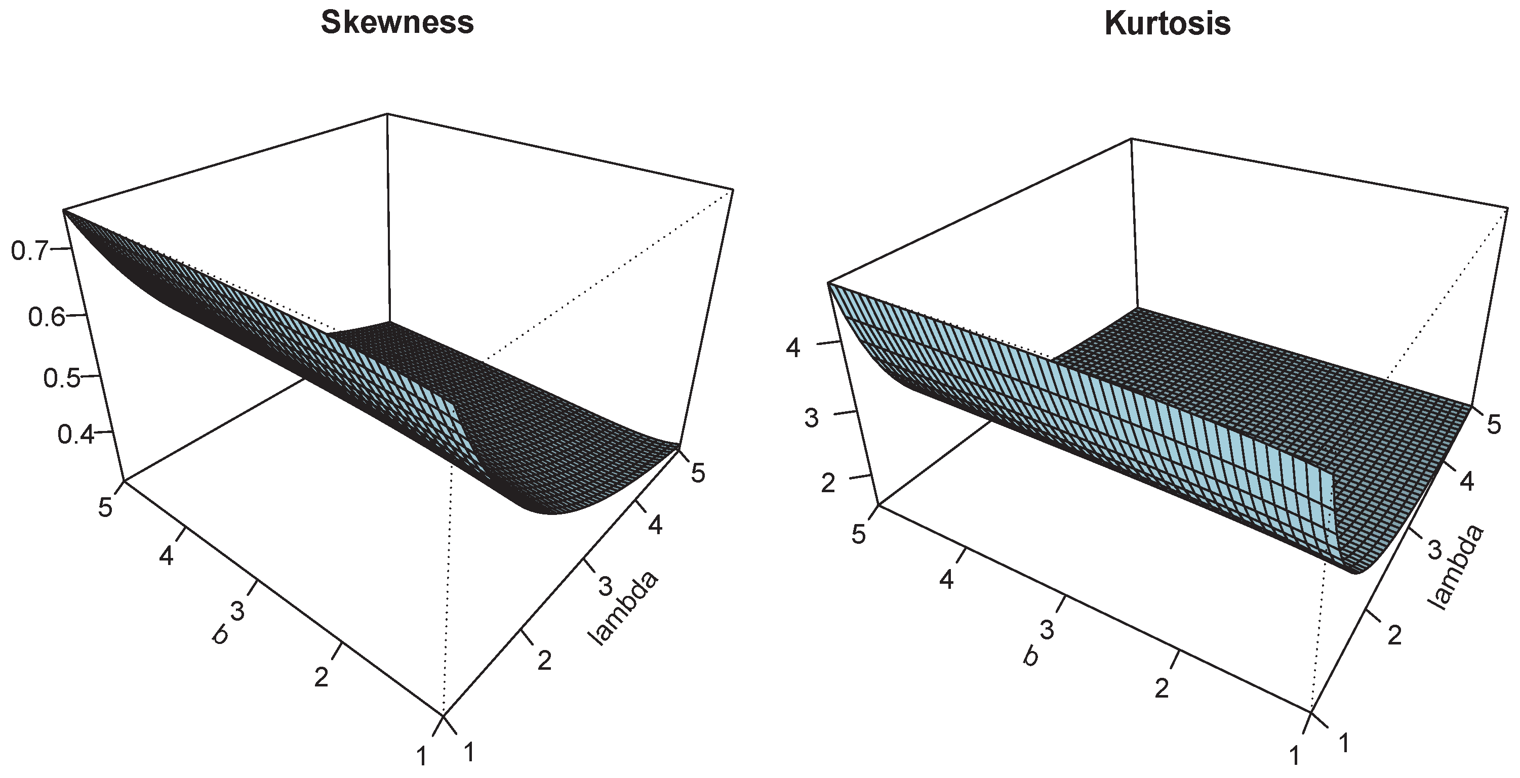
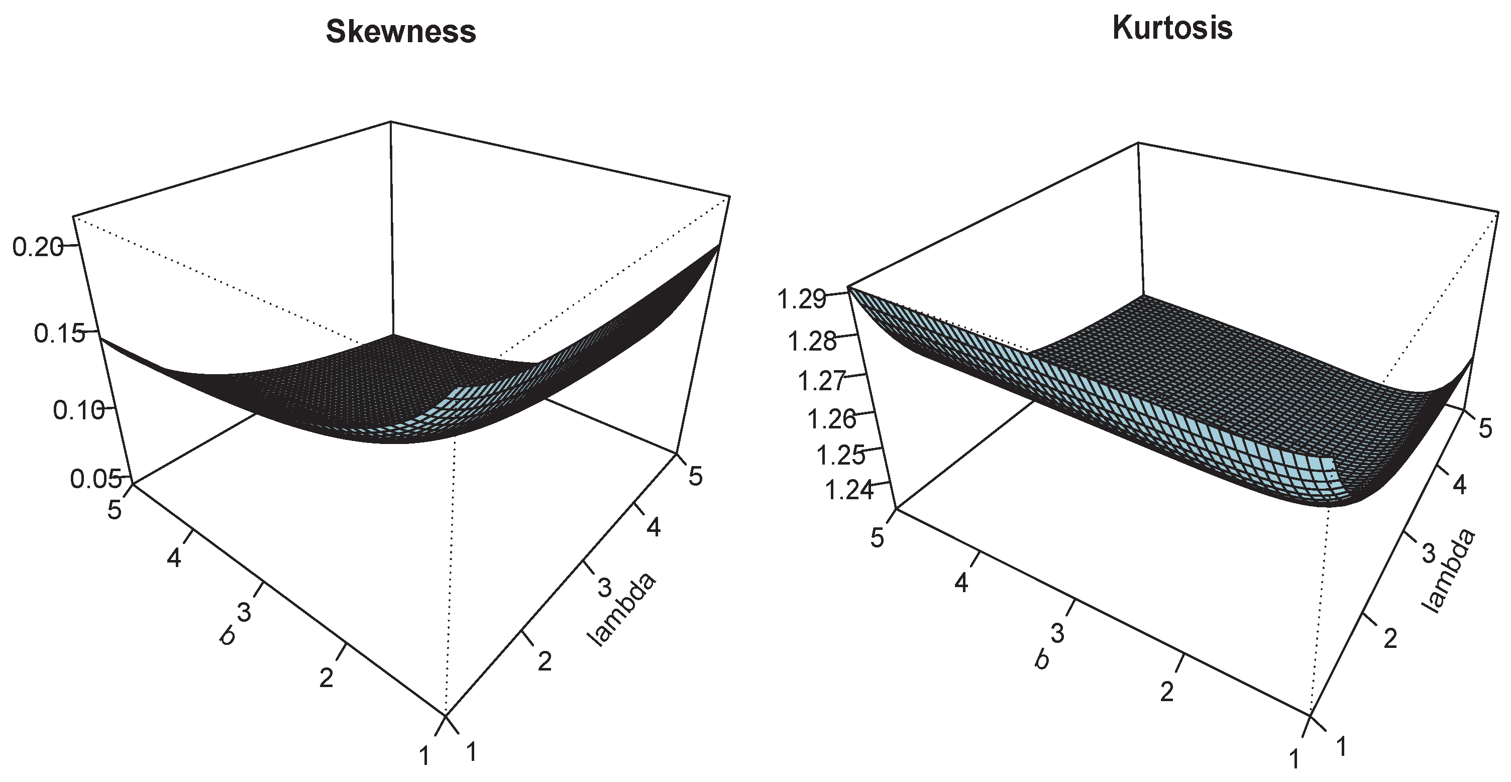
Figure 4.
Plots of and for and .
Figure 4.
Plots of and for and .
Figure 5.
Plots of and for and .
Figure 5.
Plots of and for and .
Figure 6.
Plots of and for and .
Figure 6.
Plots of and for and .
Figure 7.
Plots of and for and .
Figure 7.
Plots of and for and .
Figure 8.
Plots of and for and .
Figure 8.
Plots of and for and .
Figure 9.
Total test time (TTT) plot and boxplot for data set 1.
Figure 9.
Total test time (TTT) plot and boxplot for data set 1.
Figure 10.
TTT plot and boxplot for data set 2.
Figure 10.
TTT plot and boxplot for data set 2.
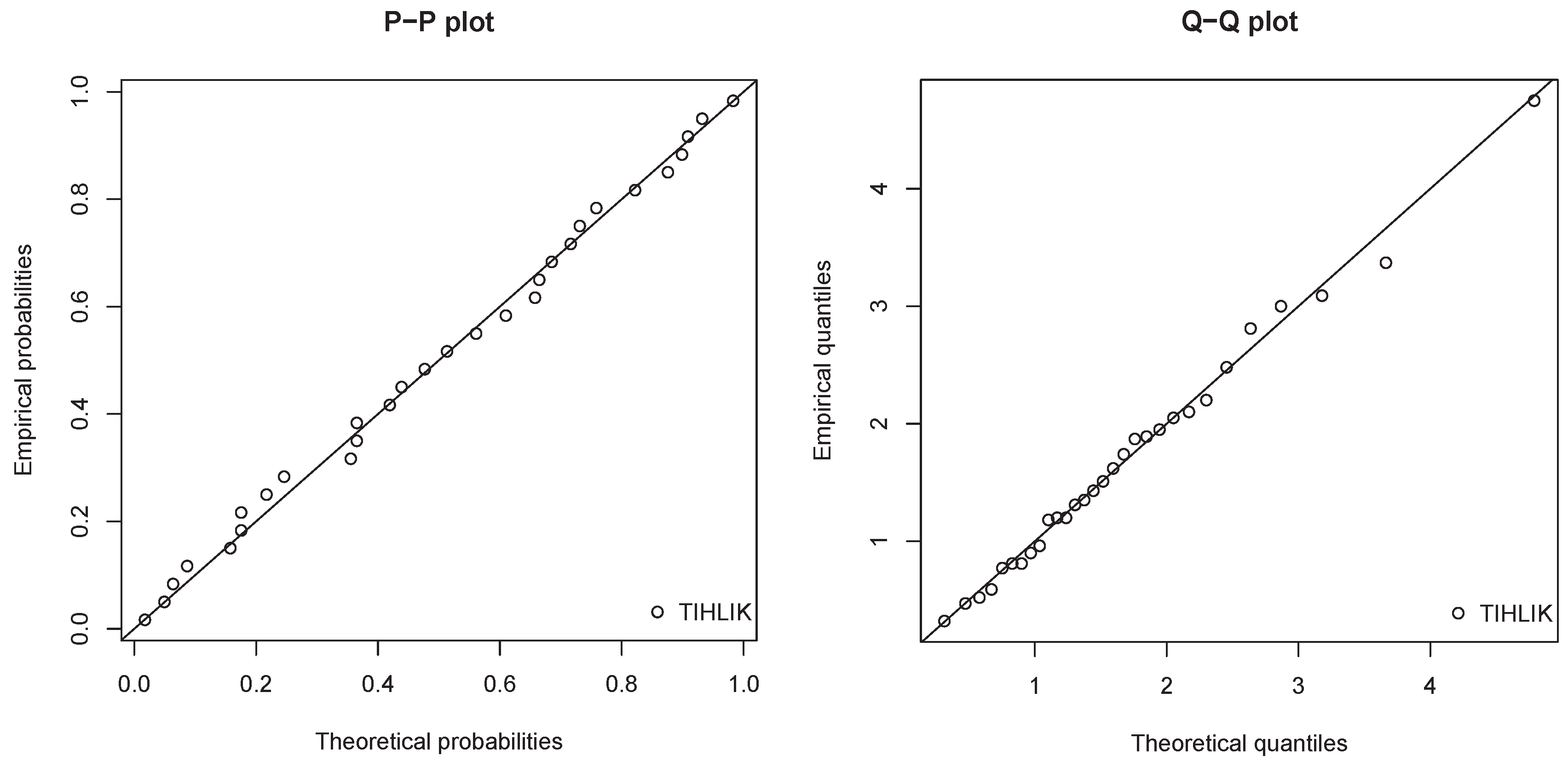
Figure 11.
Probability–Probability (P–P) plots and Quantile–Quantile (Q–Q) plot of the estimated TIHLIK model for data set 1.
Figure 11.
Probability–Probability (P–P) plots and Quantile–Quantile (Q–Q) plot of the estimated TIHLIK model for data set 1.
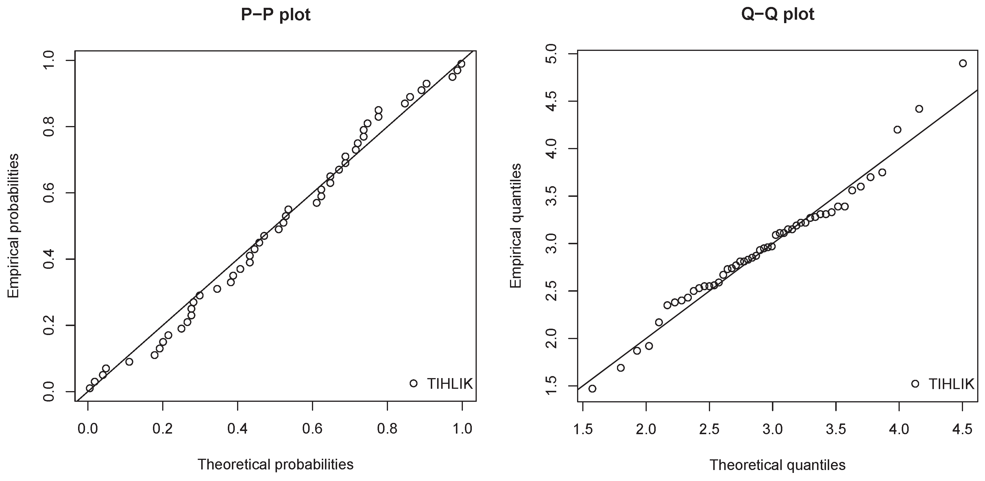
Figure 12.
P–P plot and Q–Q plot of the estimated TIHLIK model for data set 2.
Figure 12.
P–P plot and Q–Q plot of the estimated TIHLIK model for data set 2.
Figure 13.
Plots of the estimated pdfs for data set 1.
Figure 13.
Plots of the estimated pdfs for data set 1.
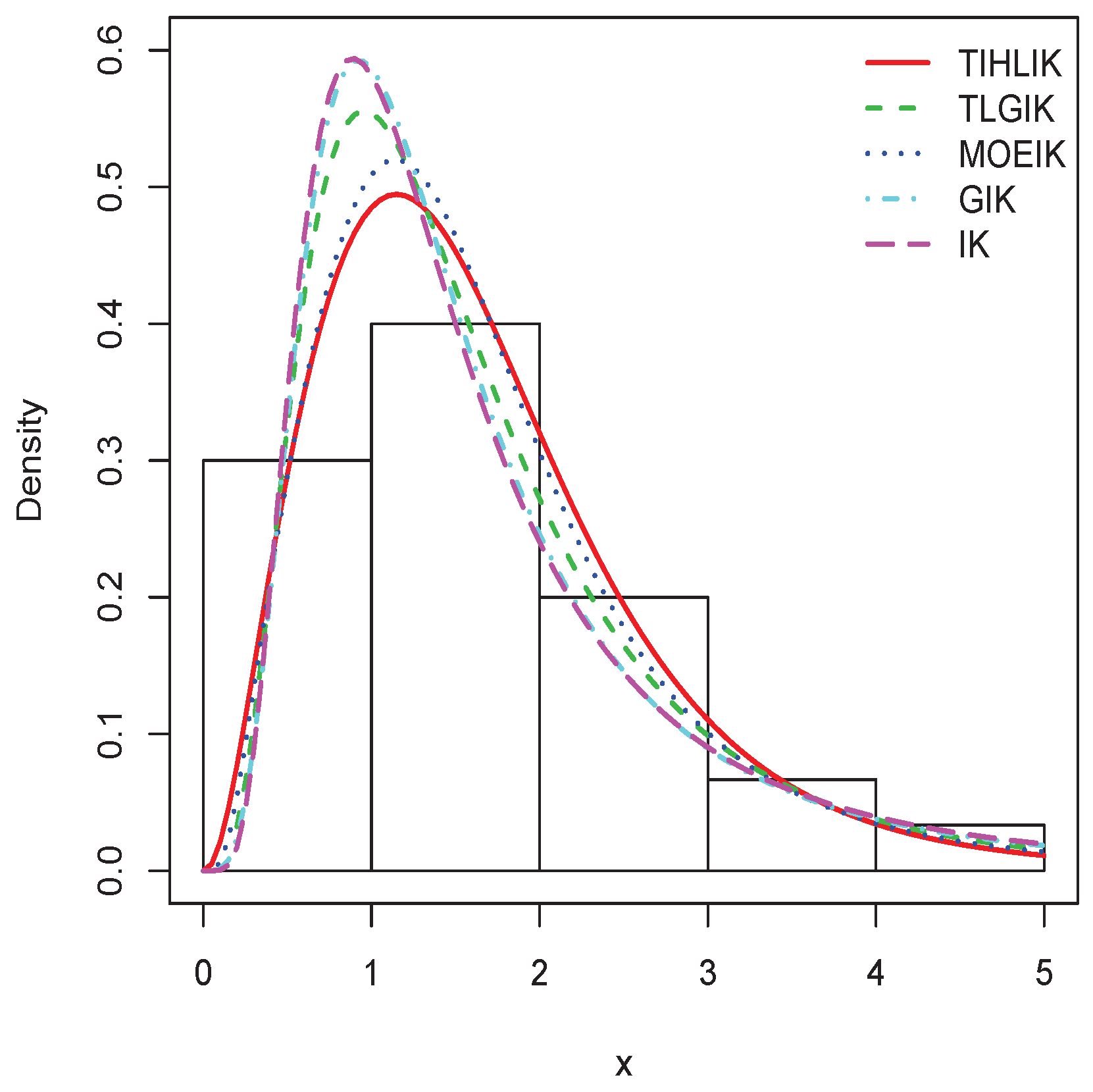
Figure 14.
Plots of the estimated pdfs for data set 2.
Figure 14.
Plots of the estimated pdfs for data set 2.
Table 1.
Some moments and variance of X for the following parameters values respecting the order ; (i): , (ii): , (iii): (iv): (v): , and (vi): .
Table 1.
Some moments and variance of X for the following parameters values respecting the order ; (i): , (ii): , (iii): (iv): (v): , and (vi): .
| (i) | (ii) | (iii) | (iv) | (v) | (vi) |
|---|
| 0.6117 | 0.8889 | 0.5127 | 0.3666 | 0.6484 | 0.2026 |
| 0.6083 | 1.1716 | 0.3594 | 0.1716 | 0.49172 | 0.0461 |
| 0.9516 | 2.2852 | 0.3326 | 0.0982 | 0.4289 | 0.0116 |
| 2.5250 | 0.2515 | 0.4065 | 0.06761 | 0.42739 | 0.0031 |
| 0.2342 | 0.3814 | 0.09652 | 0.0372 | 0.0712 | 0.0050 |
Table 2.
Estimates and mean square errors (MSEs) of TIHLIK model for maximum likelihood (ML), least squares (LS), weighted least square (WLS), Cramer-von Mises minimum distance (CV), and right-tail Anderson–Darling (RTAD) estimates for the Set1, i.e., , , .
Table 2.
Estimates and mean square errors (MSEs) of TIHLIK model for maximum likelihood (ML), least squares (LS), weighted least square (WLS), Cramer-von Mises minimum distance (CV), and right-tail Anderson–Darling (RTAD) estimates for the Set1, i.e., , , .
| MLE | LSE | WLSE | CVE | RTADE |
|---|
| n | Est. | MSEs | Est. | MSEs | Est. | MSEs | Est. | MSEs | Est. | MSEs |
|---|
| 30 | 1.628 | 0.043 | 1.473 | 0.259 | 1.581 | 2.084 | 1.562 | 0.459 | 1.473 | 0.319 |
| 1.950 | 0.102 | 2.296 | 0.763 | 2.329 | 0.991 | 2.395 | 0.888 | 2.450 | 1.580 |
| 2.237 | 0.492 | 2.109 | 0.551 | 2.126 | 1.188 | 2.351 | 1.018 | 2.171 | 0.851 |
| 50 | 1.603 | 0.026 | 1.550 | 0.263 | 1.616 | 0.362 | 1.575 | 0.311 | 1.547 | 0.189 |
| 1.895 | 0.070 | 2.110 | 0.588 | 2.067 | 0.600 | 2.201 | 0.708 | 2.144 | 0.639 |
| 2.144 | 0.282 | 2.049 | 0.348 | 2.094 | 0.362 | 2.169 | 0.534 | 2.088 | 0.386 |
| 100 | 1.601 | 0.015 | 1.505 | 0.137 | 1.610 | 0.242 | 1.541 | 0.151 | 1.492 | 0.128 |
| 1.900 | 0.026 | 2.162 | 0.475 | 2.031 | 0.498 | 2.172 | 0.516 | 2.241 | 0.536 |
| 2.124 | 0.095 | 2.009 | 0.120 | 2.046 | 0.148 | 2.068 | 0.131 | 2.058 | 0.139 |
Table 3.
Estimates and MSEs of TIHLIK model for ML, LS, WLS, CV, and RTAD estimates for the Set2, i.e., , , .
Table 3.
Estimates and MSEs of TIHLIK model for ML, LS, WLS, CV, and RTAD estimates for the Set2, i.e., , , .
| MLE | LSE | WLSE | CVE | RTADE |
|---|
| n | Est. | MSEs | Est. | MSEs | Est. | MSEs | Est. | MSEs | Est. | MSEs |
|---|
| 30 | 1.808 | 0.074 | 1.688 | 0.324 | 1.834 | 0.646 | 1.775 | 0.310 | 1.757 | 0.297 |
| 2.344 | 0.187 | 2.672 | 1.429 | 2.618 | 1.718 | 2.766 | 1.604 | 2.646 | 1.264 |
| 2.058 | 0.226 | 1.951 | 0.407 | 2.052 | 0.752 | 2.142 | 0.572 | 2.020 | 0.273 |
| 50 | 1.789 | 0.073 | 1.657 | 0.320 | 1.747 | 0.399 | 1.630 | 0.320 | 1.824 | 0.227 |
| 2.325 | 0.153 | 2.726 | 1.146 | 2.719 | 1.400 | 2.893 | 1.450 | 2.524 | 0.850 |
| 2.022 | 0.207 | 1.941 | 0.167 | 2.016 | 0.213 | 2.006 | 0.258 | 2.034 | 0.247 |
| 100 | 1.803 | 0.053 | 1.672 | 0.273 | 1.715 | 0.385 | 1.621 | 0.301 | 1.786 | 0.202 |
| 2.325 | 0.131 | 2.710 | 1.142 | 2.714 | 1.383 | 2.833 | 1.286 | 2.482 | 0.728 |
| 2.025 | 0.111 | 1.942 | 0.144 | 1.956 | 0.124 | 1.960 | 0.116 | 1.968 | 0.100 |
Table 4.
Estimates and MSEs of TIHLIK model for ML, LS, WLS, CV, and RTAD estimates for the Set3, i.e., , , .
Table 4.
Estimates and MSEs of TIHLIK model for ML, LS, WLS, CV, and RTAD estimates for the Set3, i.e., , , .
| MLE | LSE | WLSE | CVE | RTADE |
|---|
| n | Est. | MSEs | Est. | MSEs | Est. | MSEs | Est. | MSEs | Est. | MSEs |
|---|
| 30 | 1.869 | 0.186 | 1.715 | 0.419 | 1.753 | 0.469 | 1.778 | 0.355 | 1.835 | 0.304 |
| 2.435 | 0.410 | 2.834 | 0.939 | 2.940 | 2.095 | 2.942 | 0.944 | 2.699 | 1.218 |
| 2.278 | 0.547 | 2.193 | 0.716 | 2.186 | 0.861 | 2.305 | 0.614 | 2.258 | 0.846 |
| 50 | 1.856 | 0.152 | 1.616 | 0.215 | 1.827 | 0.458 | 1.685 | 0.233 | 1.851 | 0.345 |
| 2.394 | 0.407 | 2.876 | 0.627 | 2.743 | 1.126 | 2.973 | 0.759 | 2.621 | 0.836 |
| 2.186 | 0.201 | 2.047 | 0.265 | 2.219 | 0.409 | 2.193 | 0.336 | 2.254 | 0.421 |
| 100 | 1.850 | 0.132 | 1.581 | 0.155 | 1.804 | 0.410 | 1.674 | 0.197 | 1.721 | 0.173 |
| 2.388 | 0.393 | 2.957 | 0.598 | 2.709 | 1.072 | 2.934 | 0.683 | 2.747 | 0.661 |
| 2.147 | 0.109 | 2.032 | 0.119 | 2.092 | 0.133 | 2.145 | 0.205 | 2.095 | 0.118 |
Table 5.
Estimates and MSEs of TIHLIK model for ML, LS, WLS, CV, and RTAD estimates for the Set4, i.e., , , .
Table 5.
Estimates and MSEs of TIHLIK model for ML, LS, WLS, CV, and RTAD estimates for the Set4, i.e., , , .
| MLE | LSE | WLSE | CVE | RTADE |
|---|
| n | Est. | MSEs | Est. | MSEs | Est. | MSEs | Est. | MSEs | Est. | MSEs |
|---|
| 30 | 1.810 | 0.110 | 1.751 | 0.358 | 1.753 | 0.554 | 1.775 | 0.326 | 1.839 | 0.399 |
| 2.400 | 0.503 | 2.673 | 1.243 | 2.925 | 1.393 | 2.959 | 1.702 | 2.746 | 2.197 |
| 3.456 | 0.973 | 3.171 | 1.150 | 3.330 | 1.014 | 3.515 | 1.673 | 3.350 | 1.164 |
| 50 | 1.833 | 0.124 | 1.561 | 0.165 | 1.671 | 0.344 | 1.742 | 0.252 | 1.737 | 0.253 |
| 2.409 | 0.447 | 3.021 | 1.218 | 2.925 | 1.063 | 2.916 | 1.430 | 2.849 | 1.066 |
| 3.408 | 0.633 | 3.074 | 0.740 | 3.183 | 0.747 | 3.502 | 1.379 | 3.398 | 0.862 |
| 100 | 1.825 | 0.111 | 1.586 | 0.199 | 1.692 | 0.283 | 1.539 | 0.112 | 1.681 | 0.173 |
| 2.357 | 0.454 | 2.964 | 0.698 | 2.836 | 0.906 | 3.123 | 0.632 | 2.848 | 0.730 |
| 3.346 | 0.307 | 3.090 | 0.570 | 3.169 | 0.362 | 3.117 | 0.340 | 3.260 | 0.379 |
Table 6.
Descriptive statistics for data sets 1 and 2, respectively.
Table 6.
Descriptive statistics for data sets 1 and 2, respectively.
| n | Mean | Median | Standard Deviation | Skewness | Kurtosis |
|---|
| Data set 1 | 30 | 1.68 | 1.47 | 1.00 | 1.03 | 0.93 |
| Data set 2 | 50 | 2.95 | 2.94 | 0.64 | 0.4 | 1.02 |
Table 7.
MLEs along with their standard errors (in parentheses) for data set 1.
Table 7.
MLEs along with their standard errors (in parentheses) for data set 1.
| Model | a | b | | | | | |
|---|
| TIHLIK | 0.6888 | 3.3437 | 13.5822 | - | - | - |
| (0.4690) | (0.2944) | (0.6816) | - | - | - |
| TLGIK | - | - | 1.2334 | 1.9057 | 21.3625 | 0.2051 |
| - | - | (0.9359) | (1.5024) | (3.8678) | (0.3058) |
| MOEIK | - | - | 6.8751 | 4.3210 | 6.6101 | - |
| - | - | (3.5056) | (0.9386) | (2.9989) | - |
| GIK | - | - | | 3.9515 | 1.9557 | 1.4199 |
| - | - | | (3.7014) | (1.8132) | (1.0215) |
| IK | 2.9874 | 8.5913 | - | - | - | - |
| (0.4730) | (3.1230) | - | - | - | - |
Table 8.
MLEs along with their standard errors (in parentheses) for data set 2.
Table 8.
MLEs along with their standard errors (in parentheses) for data set 2.
| Model | a | b | | | | | |
|---|
| TIHLIK | 1.7115 | 33.0611 | 30.6921 | - | - | - |
| (0.5412) | (1.3753) | (0.8705) | - | - | - |
| TLGIK | - | - | 1.7205 | 2.0776 | 63.2200 | 1.1643 |
| - | - | (0.8203) | (1.1502) | (4.8377) | (1.1403) |
| MOEIK | - | - | 29.7926 | 5.3374 | 41.9828 | - |
| - | - | (17.8294) | (0.4872) | (20.7064) | - |
| GIK | - | - | | 8.7194 | 15.7859 | 0.3478 |
| - | - | | (6.3860) | (4.2844) | (0.2559) |
| IK | 3.1501 | 51.0099 | - | - | - | - |
| (0.2359) | (14.4844) | - | - | - | - |
Table 9.
The , AIC, BIC, W, A, KS, and p-value values for data set 1.
Table 9.
The , AIC, BIC, W, A, KS, and p-value values for data set 1.
| Model | | AIC | BIC | W | A | KS | p-Value (KS) |
|---|
| TIHLIK | 38.1741 | 82.3483 | 83.2714 | 0.0144 | 0.1055 | 0.0575 | 0.9999 |
| TLGIK | 38.5302 | 85.0605 | 90.6653 | 0.0302 | 0.1943 | 0.0932 | 0.9566 |
| MOEIK | 38.3427 | 82.6855 | 86.8891 | 0.0196 | 0.1349 | 0.0679 | 0.9871 |
| GIK | 39.3172 | 84.6345 | 88.8381 | 0.0514 | 0.3226 | 0.1097 | 0.8628 |
| IK | 39.4255 | 83.2954 | 85.6534 | 0.0561 | 0.3505 | 0.1143 | 0.8279 |
Table 10.
The , AIC, BIC, W, A, KS, and p-value values for data set 2.
Table 10.
The , AIC, BIC, W, A, KS, and p-value values for data set 2.
| Model | | AIC | BIC | W | A | KS | p-Value (KS) |
|---|
| TIHLIK | 47.3670 | 100.7342 | 106.4702 | 0.0616 | 0.4354 | 0.0879 | 0.8338 |
| TLGIK | 51.8215 | 111.6431 | 119.2911 | 0.1941 | 1.2270 | 0.1153 | 0.5189 |
| MOEIK | 61.4733 | 128.9467 | 134.6828 | 0.0737 | 0.5004 | 0.2589 | 0.0205 |
| GIK | 61.0390 | 128.0782 | 133.81421 | 0.3163 | 1.9228 | 0.1926 | 0.0488 |
| IK | 68.3343 | 140.6686 | 144.4927 | 0.1668 | 1.0619 | 0.2548 | 0.0030 |


