A New Family of Chaotic Systems with Different Closed Curve Equilibrium

Abstract

Chaotic systems with hidden attractors, infinite number of equilibrium points and different closed curve equilibrium have received much attention in the past six years. In this work, we introduce a new family of chaotic systems with different closed curve equilibrium. Using the methods of equilibrium points, phase portraits, maximal Lyapunov exponents, Kaplan–Yorke dimension, and eigenvalues, we analyze the dynamical properties of the proposed systems and extend the general knowledge of such systems.

1. Introduction

Over the past fifty years, investigating chaotic systems has attracted many researchers’ attention. Generating chaotic attractors may help one to understand the dynamics of the real system. Recently, new chaotic systems with hidden attractors have been introduced [1,2]. An attractor is called self-excited if its basin of attraction intersects any open neighborhood of a stationary state (an equilibrium), otherwise it is called a hidden attractor. It is generally accepted that there are three main families of hidden attractors [1,3,4]: hidden attractors with stable equilibria, hidden attractors without equilibrium and hidden attractors with infinite number of equilibrium points. Some developments include chaotic systems without any equilibrium points [5,6,7,8,9,10], with a single stable equilibrium [11,12], and with uncountable equilibria [13,14,15]. However, there is little discussion on systems with different families of hidden attractors [4,16]. Undoubtedly, many undiscovered systems surely exist. In this study, the authors present a family of chaotic systems with different closed curve equilibriums, being the promotion of published papers, which may extend the general knowledge of such systems.

Gotthans and Petr$\check{z}$ela [14] have introduced a general three-dimensional model generating hidden attractors with infinite equilibria. The model is given as:

$$\begin{array}{cc}\hfill \dot{x}& =z,\hfill \\ \hfill \dot{y}& =z{g}_1(x,y,z),\hfill \\ \hfill \dot{z}& =g_2(x,y,z),\hfill \end{array}$$

(1)

where x, y and z are state variables, while $g_1(x,y,z)$ and $g_2(x,y,z)$ are two nonlinear functions.

Motivated by the works mentioned above, in this paper, we introduce and investigate a new family of chaotic systems with different closed curve equilibriums. Replacing $g_1(x,y,z)$ with $ay+b{y}^2+xz$, and $g_2(x,y,z)$ with ${\left|x\right|}^k+{\left|y\right|}^k-1$ in (1), i.e.,

$$\begin{array}{cc}\hfill g_1(x,y,z)& =ay+b{y}^2+xz,\hfill \\ \hfill g_2(x,y,z)& ={\left|x\right|}^k+{\left|y\right|}^k-1,\hfill \end{array}$$

(2)

the proposed novel system is obtained as

$$\begin{array}{cc}\hfill \dot{x}& =z,\hfill \\ \hfill \dot{y}& =-z(ay+b{y}^2+xz),\hfill \\ \hfill \dot{z}& ={\left|x\right|}^k+{\left|y\right|}^k-1,\hfill \end{array}$$

(3)

where a and b are both positive parameters, while k is a positive integer. In fact, the new model (3) contains several known systems as special cases.

• $(Example$$A)$
  For the case of $k=2$, system (3) corresponds to the following system:

  $$\begin{array}{cc}\hfill \dot{x}& =z,\hfill \\ \hfill \dot{y}& =-z(ay+b{y}^2+xz),\hfill \\ \hfill \dot{z}& =x^2+y^2-1.\hfill \end{array}$$

  (4)

  Actually, model (4) was studied by Gotthans and Petr$\check{z}$ela in [15] and has shown that there exists some chaotic system with a circle of equilibrium points as $\left\{(x,y,0):x^2+y^2=1\right\}$.
• $(Example$$B)$
  For the case of $k=4$, system (3) corresponds to the following system:

  $$\begin{array}{cc}\hfill \dot{x}& =z,\hfill \\ \hfill \dot{y}& =-z(ay+b{y}^2+xz),\hfill \\ \hfill \dot{z}& =x^4+y^4-1.\hfill \end{array}$$

  (5)

  Model (5) is exactly the system studied by Pham et al. in [4] and have been shown that there exists a chaotic system with a rounded square equilibrium as $\left\{(x,y,0):x^4+y^4=1\right\}$.

Above all, the aim of this study is to introduce a new family of chaotic systems generating hidden attractors with differently shaped equilibrium points, containing systems (4) and (5) as two particular cases, being the generalization of the existing results, and to broaden the views on the hidden attractors.

For any integer k, by solving the following system

$$\left\{\begin{array}{c}z=0,\hfill \\ -z(ay+b{y}^2+xz)=0,\hfill \\ {\left|x\right|}^k+{\left|y\right|}^k-1=0,\hfill \end{array}\right.$$

(6)

we obtain the equilibrium points of system (3). It is easy to see that the proposed system (3) has a family of different curve equilibriums of $\left\{(x,y,0):{\left|x\right|}^k+{\left|y\right|}^k=1\right\}$, as illustrated in Figure 1. With the increasing values of k, the area covered by the different closed curves ${\left|x\right|}^k+{\left|y\right|}^k=1$ is getting larger.

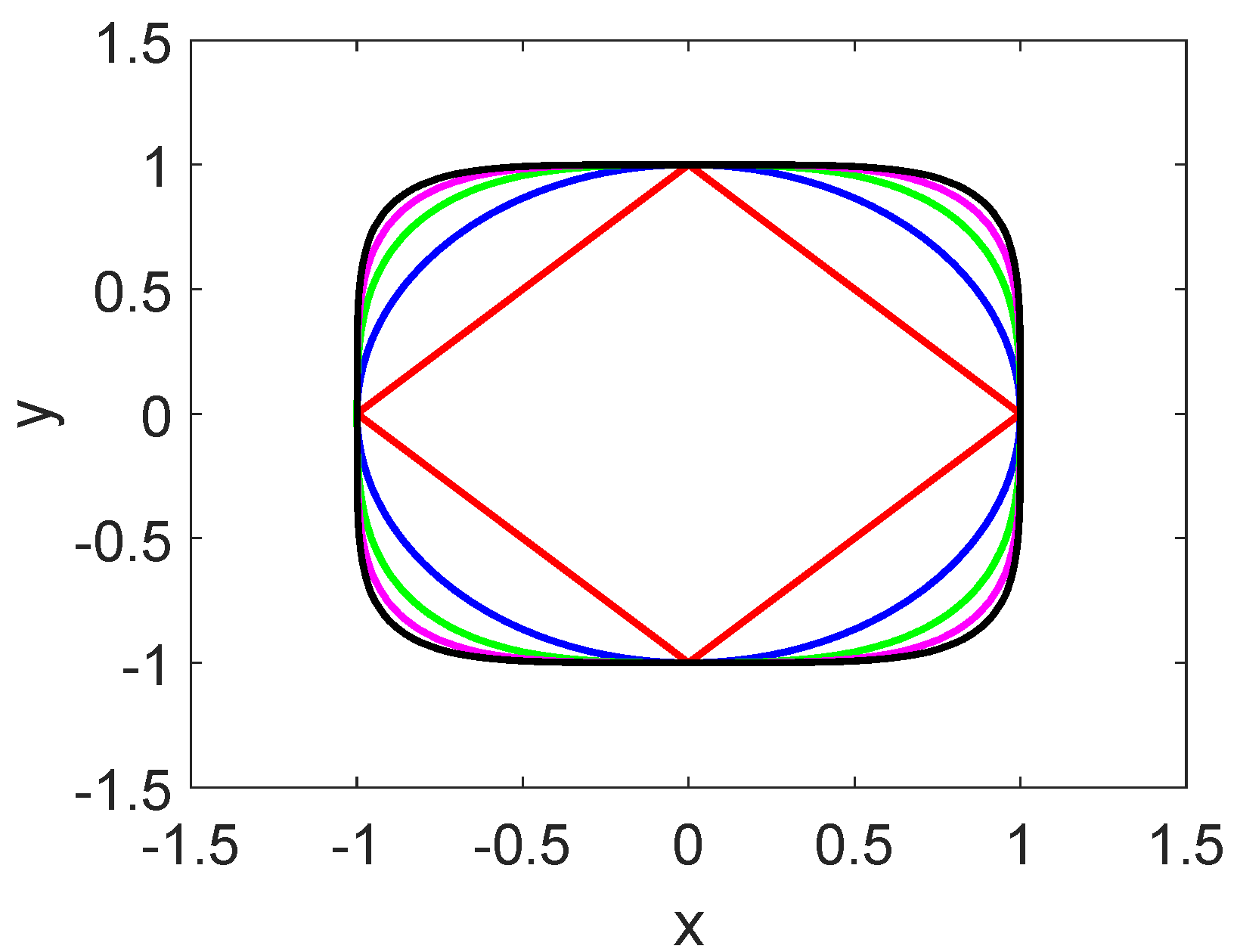
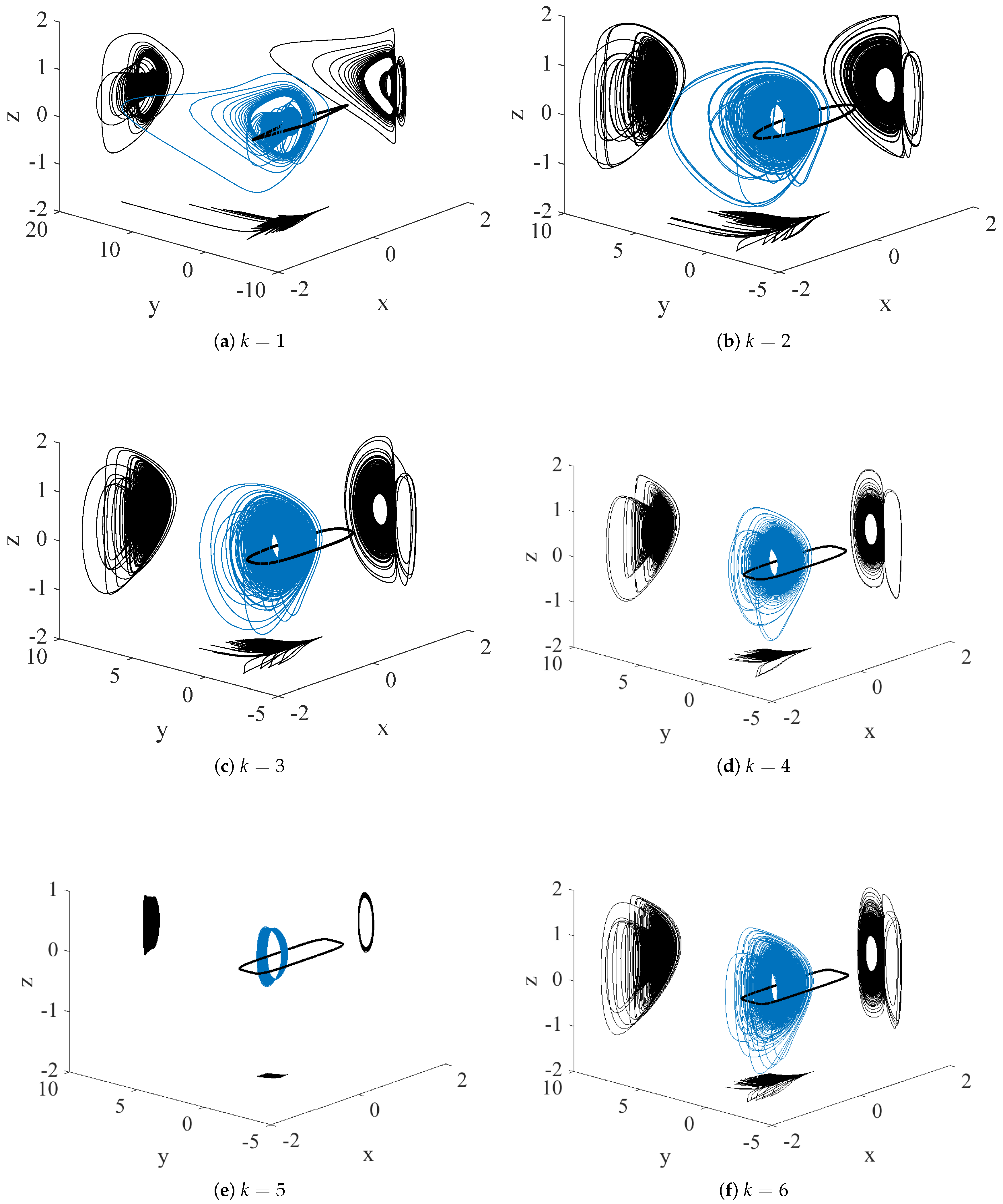
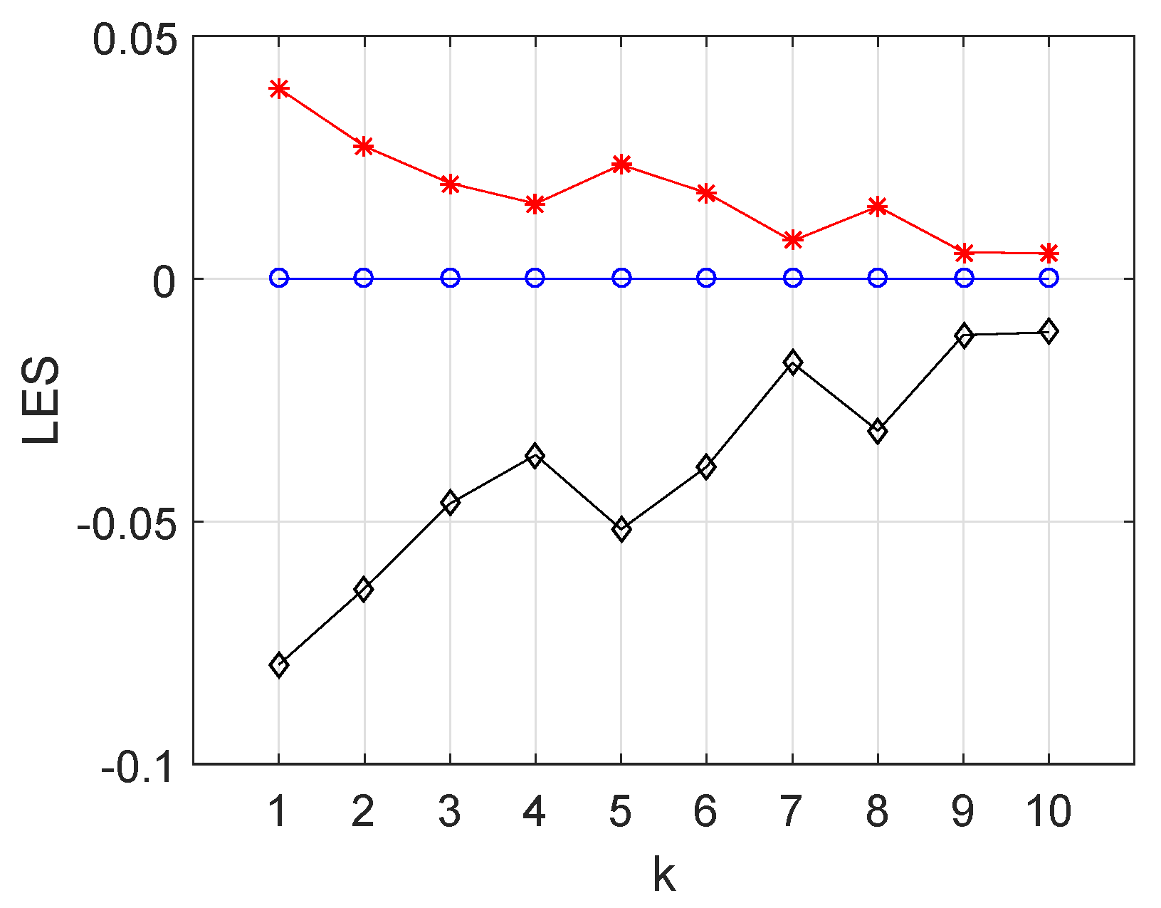
2. Chaotic Behavior of the Proposed System

Consider a general n-dimensional autonomous vector field

$$\dot{x}=f\left(x\right),x\in {\mathbb{R}}^n.$$

(7)

An equilibrium solution of (7) is a point $x^{\ast }\in {\mathbb{R}}^n$ such that $f\left(x^{\ast }\right)=0$, i.e., a solution which does not change in time. Other terms substituted for the term equilibrium solution are fixed point or critical point. In order to determine the stability of $x^{\ast },$ we must understand the nature of solution near $x^{\ast }$. We do this by linearzing (7) at $x^{\ast }$, that is, by studying the following linear system

$$\dot{\xi }=Df\left(x^{\ast }\right)\xi ,\xi \in {\mathbb{R}}^n,$$

(8)

where $Df=[\partial f_i/\partial x_j]$ is the Jacobian matrix of first partial derivatives of the function $f={(f_1(x_1,\dots ,x_n),f_2(x_1,\dots ,x_n),\dots ,f_n(x_1,\dots ,x_n))}^T$ (T denotes transpose), and $x=x^{\ast }+\xi$.

An equilibrium is called $hyperbolic$ if there are no eigenvalues of $Df\left(x\right)$ on the imaginary axis. The following well-known theorem for hyperbolic equilibrium is very crucial in this paper.

Theorem 1.

[17] Suppose that all of the eigenvalues of $Df\left(x^{\ast }\right)$ have negative real parts. Then, the equilibrium solution $x=x^{\ast }$ of the nonlinear vector field is asymptotically stable.

However, it is worth mentioning that the situation is very complicated for the nonhyperbolic equilibrium. Let us recall some definitions that are well known in the literature.

Definition 1.

[18] An attractor is a minimal closed invariant set that attracts nearby trajectories lying in the domain of stability (or basin of attraction) onto it.

Definition 2.

[18] A chaotic attractor is an attractor that exhibits sensitivity to initial conditions.

Definition 3.

[18] The spectrum of Lyapunov exponents are quantities that characterize the rate of separation of infinitesimally close trajectories.

Chaos is a phenomenon that is not easily identified or classified. There is also no universally accepted definitions for chaos, but there are some characteristics displayed by the solutions of chaotic systems: sensitivity to initial conditions; long-term nonperiodic behavior and fractal structure. Generally, a system is chaotic if at least one of the Lyapunov exponents is positive. This implies that two trajectories that start initially close to each other on the strange attractor will diverge as time increases.

It is worthwhile to note that system (3) with a family of different curve equilibrium points displays chaotic attractors (see Figure 2) for $a=5,b=3$, and the initial conditions $\left(x\right(0),y(0),z(0\left)\right)=(0,0,0)$. The black closed contour in the middle of each of Figure 2a–f is the plot of the closed curve equilibrium for the different values of k, respectively. Chaotic behavior of the system is generally confirmed by the Lyapunov exponents calculated by the Wolf method and the Kaplan–Yorke dimension $D_{KY}$ (see

Table 1. Lyapunov exponents of the system (3) for the value of k from 1 to 7.

Equations	Equilibrium	LEs	${\mathit{D}}_{\mathit{KY}}$
$k=1$	$\left|x^{\ast }\right|+\left|y^{\ast }\right|=1$	$(0.0392,0,-0.0795)$	$2.4931$
$k=2$	${\left(x^{\ast }\right)}^2+{\left(y^{\ast }\right)}^2=1$	$(0.0273,0,-0.0638)$	$2.4279$
$k=3$	${\left|x^{\ast }\right|}^3+{\left|y^{\ast }\right|}^3=1$	$(0.0197,0,-0.0463)$	$2.4255$
$k=4$	${\left(x^{\ast }\right)}^4+{\left(y^{\ast }\right)}^4=1$	$(0.0155,0,-0.0363)$	$2.4270$
$k=5$	${\left|x^{\ast }\right|}^5+{\left|y^{\ast }\right|}^5=1$	$(0.0235,0,-0.0516)$	$2.4554$
$k=6$	${\left(x^{\ast }\right)}^6+{\left(y^{\ast }\right)}^6=1$	$(0.0177,0,-0.0387)$	$2.4574$
$k=7$	${\left|x^{\ast }\right|}^7+{\left|y^{\ast }\right|}^7=1$	$(0.0078,0,-0.0173)$	$2.4508$

and Figure 3). In simulation, the fourth-order Runge–Kutta integration method has been used with a final time of 10,000 and the time step equals $0.01$. The results are very interesting that, with the increasing values of k, the corresponding largest Lyapunov exponents have a trend of decreasing.

Dynamical motion in the close neighborhood of the equilibrium is determined by the eigenvalues and associated eigenspace established along this structure [14,15]. The partial derivatives of the state variables are required in estimating the Jacobian matrix. The derivation of $\left|·\right|$ can be obtained in several ways. Here, $sgn(·)$ is the signum function. It is known that the signum function is not differentiable at 0.

In the case of the system (3), a state-dependent linearization matrix is easily established as

$$J_{(x,y,z)}=D{f}_{(x,y,z)}=\left(\begin{array}{ccc}0& 0& 1\\ -z^2& -az-2byz& -2xz-ay-b{y}^2\\ k{x}^{k-1}{\left[sgn\left(x\right)\right]}^k& k{y}^{k-1}{\left[sgn\left(y\right)\right]}^k& 0\end{array}\right).$$

(9)

The equilibrium points lie in the plane $z=0$, so we have

$$J_{(x,y,0)}=\left(\begin{array}{ccc}0& 0& 1\\ 0& 0& -ay-b{y}^2\\ k{x}^{k-1}{\left[sgn\left(x\right)\right]}^k& k{y}^{k-1}{\left[sgn\left(y\right)\right]}^k& 0\end{array}\right).$$

(10)

The local behavior along the equilibrium is determined by the eigenvalues, i.e., the roots of the characteristic equation

$$Det(J_{(x,y,0)}-\lambda E)=-\lambda [{\lambda }^2+k{y}^{k-1}{\left[sgn\left(y\right)\right]}^k(ay+b{y}^2)-k{x}^{k-1}{\left[sgn\left(x\right)\right]}^k]=0.$$

(11)

The eigenvalues are given by

$$\begin{array}{cc}\hfill {\lambda }_1& =0,\hfill \\ \hfill {\lambda }_{2,3}& =\pm {(k{x}^{k-1}{\left[sgn\left(x\right)\right]}^k-k{y}^{k-1}{\left[sgn\left(y\right)\right]}^k(ay+b{y}^2))}^{\frac{1}{2}}.\hfill \end{array}$$

(12)

Particularly, for $k=1$, we have (See

Table 2. Eigenvalues of the system (3) for $k=1$.

Case	${\mathit{\lambda }}_{2,3}$
I     $0<y<0.1805$	one positve real, one negative real
I     $0.1805<y<1$	a pair of purely imaginary
$II$	a pair of purely imaginary
$III$	a pair of purely imaginary
$IV$   $-1<y<-0.2324$	a pair of purely imaginary
$IV$   $-0.2324<y<0$	one positve real, one negative real
$x=0,y=1$	${\lambda }_{2,3}=\pm 2.8284i$
$x=-1,y=0$	${\lambda }_{2,3}=\pm i$
$x=0,y=-1$	${\lambda }_{2,3}=\pm 1.4142i$
$x=1,y=0$	${\lambda }_{2,3}=\pm 1$
$x=0.8195,y=0.1805$	${\lambda }_{2,3}=0$
$x=0.7676,y=-0.2324$	${\lambda }_{2,3}=0$

)

$$\begin{array}{cc}\hfill {\lambda }_1& =0,\hfill \\ \hfill {\lambda }_{2,3}& =\pm {(sgn\left(x\right)-sgn\left(y\right)(ay+b{y}^2))}^{\frac{1}{2}}.\hfill \end{array}$$

(13)

Particularly, for $k=2$, we have (See

Table 3. Eigenvalues of the system (3) for $k=2$.

Case	${\mathit{\lambda }}_{2,3}$
I   $0.9221<x<1,0<y<0.3869$	one positve real, one negative real
I   $0<x<0.9221,y>0.3869$	a pair of purely imaginary
$II$	a pair of purely imaginary
$III$	a pair of purely imaginary
$IV$   $0.8676<x<1,-0.4973<y<0$	a pair of purely imaginary
$IV$   $0<x<0.8676,-1<y<-0.4973$	one positve real, one negative real
$x=0,y=1$	${\lambda }_{2,3}=\pm 4i$
$x=-1,y=0$	${\lambda }_{2,3}=\pm 1.4142i$
$x=0,y=-1$	${\lambda }_{2,3}=\pm 2i$
$x=1,y=0$	${\lambda }_{2,3}=\pm 1.4142$
$x=0.8676,y=0.4973$	${\lambda }_{2,3}=0$
$x=0.9221,y=0.3869$	${\lambda }_{2,3}=0$

)

$$\begin{array}{cc}\hfill {\lambda }_1& =0,\hfill \\ \hfill {\lambda }_{2,3}& =\pm {(2x-2y(ay+b{y}^2))}^{\frac{1}{2}}.\hfill \end{array}$$

(14)

In Table 2 and Table 3, I, $II$, $III$, $IV$ represent the four quadrants, respectively.

A pair of purely imaginary eigenvalues represent an unstable center equilibrium. Then, there are concentric periodic orbits around the equilibrium curves. In addition, the pair of purely real eigenvalues implies an unstable saddle. Furthermore, three-dimensional Bogdanov–Takens equilibria (${\lambda }_1={\lambda }_2={\lambda }_3=0$) are also presented for the case of $k=1,2$.

3. Conclusions

The main goal of the current study is to propose a novel and more general family of chaotic systems with different curve equilibriums located on a quadrangle, a circle or other general cases. Furthermore, the chaotic systems here are the extension of existing literature. Dynamics of the new system have been investigated via different tools such as Phase portrait, Kaplan–Yorke dimension, Maximal Lyapunov exponents, and Eigenvalues. The results in this study provide a new and in-depth understanding of such systems. Physical realization of chaotic models have been used in different applications such as chaotic masking communications [19] and autonomous robots [20]. Furthermore, the feasibility of the theoretical model can be confirmed via their realizations, which is future work.

References

1. Dudkowski, D.; Kapitaniak, T.; Kuznetsov, N.V.; Leonov, G.A.; Prasad, A. Hidden attractors in dynamical systems. Phys. Rep. 2016, 637, 1–50. [Google Scholar] [CrossRef]
2. Kuznetsov, N.I. Hidden attractors in fundamental problems and engineering models: A short survey. In AETA 2015: Recent Advances in Electrical Engineering and Related Sciences; Lecture Notes in Electrical Engineering; Duy, V., Dao, T., Zelinka, I., Choi, H.S., Chadli, M., Eds.; Springer: Cham, Switzerland, 2015; Volume 371, pp. 13–25. [Google Scholar]
3. Kapitaniak, T.; Leonov, G.A. Multistability: uncovering hidden attractors. Eur. Phys. J. Spec. Top. 2015, 224, 1405–1408. [Google Scholar] [CrossRef]
4. Pham, V.-T.; Jafari, S.; Volos, C.; Gotthans, T.; Wang, X.; Hoang, D.V. A chatoic system with rounded square equilibrium and with no-equilibrium. Optik 2017, 130, 365–371. [Google Scholar] [CrossRef]
5. Wang, X.; Chen, G. Constructing a chaotic system with any number of equilibria. Nonlinear Dyn. 2013, 71, 429–436. [Google Scholar] [CrossRef]
6. Wei, Z. Dynamical behaviors of a chaotic system with no equilibria. Phys. Lett. 2011, 376, 102–108. [Google Scholar] [CrossRef]
7. Wei, Z.; Wang, R.; Liu, A. A new finding of the existence of hidden hyperchaotic attractor with no equilibria. Math. Comput. Simul. 2014, 100, 13–23. [Google Scholar] [CrossRef]
8. Pham, V.-T.; Volos, C.K.; Jafari, S.; Wei, Z.; Wang, X. Constructing a novel no-equilibrium chaotic system. Int. J. Bifurc. Chaos 2014, 24, 1450073. [Google Scholar] [CrossRef]
9. Tahir, F.R.; Jafari, S.; Pham, V.-T.; Wang, X. A novel no-equilibrium chaotic system with multiwing butterfly attractors. Int. J. Bifurc. Chaos 2015, 25, 1550056. [Google Scholar] [CrossRef]
10. Pham, V.-T.; Vaidyanathan, S.; Volos, C.K.; Jafari, S.; Kingni, S.T. A no-equilibrium hyperchaotic system with a cubic nonlinear term. Optik 2016, 127, 3259–3265. [Google Scholar] [CrossRef]
11. Molaie, M.; Jafari, S.; Sprott, J.C.; Golpayegani, S. Simple chaotic flows with one stable equilibrium. Int. J. Bifurc. Chaos 2013, 23, 1350188. [Google Scholar] [CrossRef]
12. Wang, X.; Chen, G. A chaotic system with only one stable equilibrium. Commun. Nonlinear Sci. Numer. Simul. 2012, 17, 1264–1272. [Google Scholar] [CrossRef] [Green Version]
13. Jafari, S.; Sprott, J.C. Simple chaotic flows with a line equilibrium. Chaos Solitons Fractals 2013, 57, 79–84. [Google Scholar] [CrossRef]
14. Gotthans, T.; Petržela, J. New class of chaotic systems with circular equilibrium. Nonlinear Dyn. 2015, 73, 429–436. [Google Scholar] [CrossRef]
15. Gotthans, T.; Sprott, J.C.; Petržela, J. Simple chaotic flow with circle and square equilibrium. Int. J. Bifurc. Chaos 2016, 26, 1650137. [Google Scholar] [CrossRef]
16. Pham, V.-T.; Volos, C.; Jafari, S.; Vaidyanathan, S.; Kapitaniak, T.; Wang, X. A chaotic systems with different families of hidden attractors. Int. J. Bifurc. Chaos 2016, 26, 1650139. [Google Scholar] [CrossRef]
17. Wiggins, S. Linearization. In Introduction to Applied Nonlinear Dynamical Systems and Chaos, 2nd ed.; Marsden, J.E., Sirovich, L., Antman, S.S., Eds.; Springer: New York, NY, USA, 2002; pp. 10–11. [Google Scholar]
18. Lynch, S. Three-Dimensional Autonomous Systems and Chaos. In Dynamical Systems With Applications Using Matlab, 2nd ed.; Marsden, J.E., Sirovich, L., Antman, S.S., Eds.; Springer International Publishing: Dordrecht, Switzerland, 2014; pp. 294–296. [Google Scholar]
19. Cicek, S.; Ferikoglu, A.; Pehlivan, I. A new 3D chaotic system: dynamical analysis, electronic circuit design, active control synchronization and chaotic masking communication application. Optik 2016, 127, 4024–4030. [Google Scholar] [CrossRef]
20. Volos, C.; Kyprianidis, I.; Stouboulos, I. A chaotic path planning generator for autonomous mobile robots. Robot. Auton. Syst. 2012, 60, 651–656. [Google Scholar] [CrossRef]
Figure 1. Different shapes of equilibrium points of system (3), k = 1 , 2 , 3 , 4 , 5 , from the interior to the outside, respectively.
Mathematics 07 00094 g001
Figure 2. 3D perspective view and plane projections of systems for k from 1 to 6.
Mathematics 07 00094 g002
Figure 3. The graph of the three Lyapunov exponents of system (3) for the value of k from 1 to 10.
Mathematics 07 00094 g003