Abstract
The present article was developed for the economic order quantity (EOQ) inventory model under daytime, non-random, uncertain demand. In any inventory management problem, several parameters are involved that are basically flexible in nature with the progress of time. This model can be split into three different sub-models, assuming the demand rate and the cost vector associated with the model are non-randomly uncertain (i.e., fuzzy), and these may include some of the retained learning experiences of the decision-maker (DM). However, the DM has the option of revising his/her decision through the application of the appropriate key vector of the fuzzy locks in their final state. The basic novelty of the present model is that it includes a computer-based decision-making process involving flowchart algorithms that are able to identify and update the key vectors automatically. The numerical study indicates that when all parameters are assumed to be fuzzy, the double keys of the fuzzy lock provide a more accurate optimum than other methods. Sensitivity analysis and graphical illustrations are made for better justification of the model.
1. Introduction
The traditional economic order quantity (EOQ) model has been enriched with the help of modern researchers, by using a variety of approximations and methodologies to represent an uncertain world. Nash [1] started an initiative with the bargaining problem that is one of the pioneering articles in the field of decision-making for inventory management problems. In the deterministic field, it is quite outdated, but in the field of fuzzy environments, the problem itself offers some new routes in the final decision-making process.
Zadeh [2] was the first to develop the concept of the fuzzy set. Then, it was applied by Bellman and Zadeh [3] in decision-making problems. Since then, many researchers have been engaged in characterizing the actual nature of the fuzzy set [4,5,6,7,8,9]. In this context, Diamond [10,11] has discussed both k-type fuzzy numbers and star-type fuzzy numbers. A means of finding the membership of general fuzzy numbers was also developed by Chutia et al. [12]. Roychoudhury and Pedrycz [13] provided the functional relationship among fuzzy complements. In addition, fuzzy control theory was enriched by Bobylev [14,15] with the help of the Cauchy problem. Buckley [16] discussed the generalization of fuzzy sets for practical applications. To date, a number of researchers, including Roy and Maji [17], Molodtsov [18], Cagman et al. [19], etc., have studied fuzzy soft sets; fuzzy rough sets were developed by Pawlak [20], and hesitant fuzzy sets have been improved by Torra [21], Karmakar et al. [22], De and Sana [23], etc., in real-world final decision-making problems.
Moreover, the concept of integrating the impact of learning experiences into fuzzy sets, namely, the triangular dense fuzzy set (TDFS), along with new defuzzification methods, was described by De and Beg [24], and they also utilized this fuzzy set in philosophical contexts (De and Beg [25]). In their observations, the Cauchy sequence was employed, which naturally converges to zero. Using this property, they studied the triangular dense fuzzy set, in which the fuzziness decreases with time. De and Mahata [26] discussed the cloudy fuzzy set, which is an improvement to an extension of the triangular dense fuzzy set using a continuous time variable. Recently, Karmakar et al. [27,28] studied a pollution control scheme for a sponge iron production plant model utilizing the triangular dense fuzzy rule. Additionally, Maity et al. [29] developed a two-decision-makers single-decision inventory model utilizing the concept of the triangular dense fuzzy lock set.
In addition, in cases of program-based models, some recent articles should be noted Boccia et al. [30] studied a multi-commodity location-routing problem using a flow interception formulation and a branch-and-cut algorithm. Charkhgard et al. [31] discussed a linear programming algorithm to solve optimization problems with multi-linear objective functions and affine constraints. Nash et al. [32] studied a linear programming algorithm for solving primal-dual problems using linear multiplicative programs. Pelt and Fransoo [33] discussed linear programming models for a stochastic dynamic capacitated lot-sizing problem.
Thus, from the above review, it can be seen that as soon as the set operation is completed, the final decision will have been reached for final execution. However, the concept of contradiction was first introduced by De [34] through the novel research into the triangular dense fuzzy lock set (TDFLS). In this study, an EOQ model has been developed, in which the computer program conducts a comparison of numerical results obtained from different sub-models. Here, a fuzzy lock set with several key vectors—namely, single and double keys—was utilized exclusively. The organization of the rest of this article is as follows. A deterministic EOQ model with natural idle time is considered first, and the problem itself is split into three sub-models, under the assumption that the demand rate, the various cost components, and all parameters are fuzzy numbers. Then each case is studied under general fuzzy, dense fuzzy, and dense fuzzy with lock environments. For the purposes of numerical illustration, the crisp model and fuzzy models are solved separately, using LINGO software. A comparative study of the various optimum values of the objective functions is made explicitly via computational algorithm. Finally, sensitivity analysis and graphical illustration are carried out to explore the novelty of the present research.
2. Preliminaries
2.1. Triangular Dense Fuzzy Set (TDFS)
In this section, several definitions of dense fuzzy set and triangular dense fuzzy set [24] have explained with their graphical representations and examples for subsequent uses.
Definition 1.
Let à be the fuzzy number whose components are the elements ofbeing the set of real numbers and N being the set of natural numbers with the membership grade satisfying the functional relationNow asiffor somethen the set à is called dense fuzzy set. If à is triangular then it is called TDFS. Now, if for someinattains the highest membership degree 1 then the set itself is called “Normalized Triangular Dense Fuzzy Set” or NTDFS.
Example 1.
Let us assume the TDFS as follows
for0and the corresponding membership function along with the graphical illustration (Figure 1) are given by
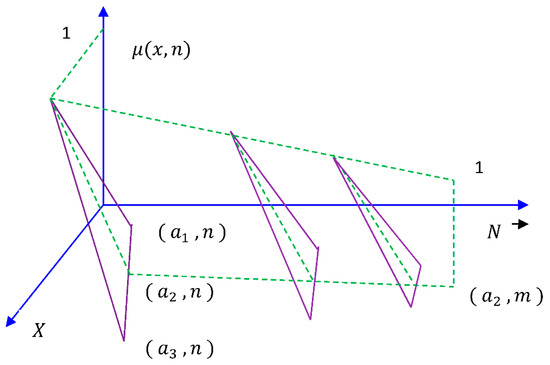
Figure 1.
Membership function of normalized triangular dense fuzzy set (NTDFS).
Remark 1.
Figure 1 shows initially the span of triangular fuzzy components are higher but as the progress of learning experiences the components become more closer and the membership degree gets near 1.
2.2. Triangular Dense Fuzzy Lock Sets (TDFLS)
Definition 2.
Letbe the TDFS whose components are the elements of, then if its membership functionsatisfies forifwith someandand in this case the index value, then the TDFSis called triangular dense fuzzy lock set (TDFLS) [34].
Definition 3.
Let the sequential definition of TDFS bewithand, whereandare the sequence of functions. Now if, ,are both converge as, then the fuzzy set does not converge to a crisp singletoni.e.,and then the TDFS becomes TDFLS.
Definition 4.
Let the sequential definition of TDFLS beforandare two Cauchy sequences of functions having converging pointsrespectively, then the fuzzy setis called triangular dense fuzzy lock set with double keys, and they depend upon ρ and σ, respectively. The corresponding membership function ofis stated in (2), and its graphical representation is given by Figure 2.
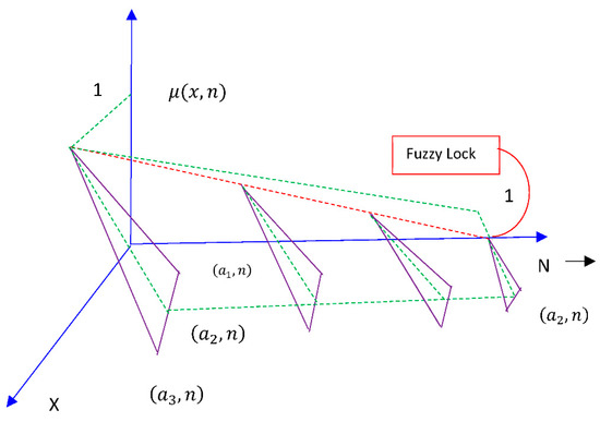
Figure 2.
Membership function of triangular dense fuzzy lock sets (TDFLS).
Remark 2.
Figure 2 shows initially the span of triangular fuzzy components are higher, but as the learning experiences progress, the components become closer and the membership degree will never reach 1.
2.3. Implication of TDFLS in Inventory Management Problems
In traditional inventory management problems, the demand rate assumes constant value from an infinite domain of instantaneous replenishment of the order quantities. However, modern research reveals that the demand rate might be non-random uncertain. Such uncertainty can be measured and gets concrete by means of learning experiences. The recent study on dense fuzzy set has been able to nullify the problem to some extent. However, though the decision-maker made a final decision prior to its application, in practice, during its process of execution, some situations arise (e.g., transportation problem, space problem, budget constraint, quantitative differences, etc.) for which the execution of the decision will have to stop instantly and consequently the decision-maker (DM) might wish to change the decision according to his/her needs. To capture the complexities of the problem the DM might have to choose the triangular dense fuzzy lock set (TDFLS) rule. With the help of TDFLS rule, any DM can overcome the problems of several parameters associated in an inventory by restricting them on lower and upper bounds immediately. Applying proper keys (which can be created from the bounds of the parameters) the DM can reach his/her expected goals.
3. Crisp Mathematical Model
Considering the needs of the present research on inventory management problems, after studying the up-to-date literature on the subject and incorporating several methodologies as preliminary concepts, the proposed mathematical model can be developed in the following way.
3.1. Assumptions and Notations
The following notations and assumptions were used to develop the model.
Notation
- Order quantity per cycle (decision variable)
- Inventory opening time per day (decision variable)
- Duration of closing/natural ideal time per day (decision variable)
- Inventory holding cost per unit quantity per day ($)
- Set up cost per cycle ($)
- Average natural idle time cost per unit idle time ($)
- selling price per unit ($)
- Cycle length (= n + 1) (days)
- Time horizon (days)
- Total average profit per cycle ($)
The definition of several costs has been added in the Appendix A.
Assumption
- Replenishments are instantaneous
- The time horizon is infinite
- The sum of opening and closing time period is unity
- Shortages are not allowed
- Holding cost is uniform over the cycle time
- Average natural idle time (leisure/pause) cost is constant per unit idle time
- The security charge, telephone charge, transportation cost (if any) etc., beyond the working hours may be considered as the idle time cost.
3.2. Formulation of the Crisp Mathematical Model
The inventory starts at the beginning of the opening time duration with inventory setup cost per cycle, holding cost per unit quantity per day and meets the demand quantity per unit time throughout the day time. After that, it remains steady up to the closing time period incurring the holding cost and idle time cost per unit idle time also. Again, it starts from the next day opening time and hence it continues up to days in similar manner. This problem can be modelled (Figure 3) in the following way:
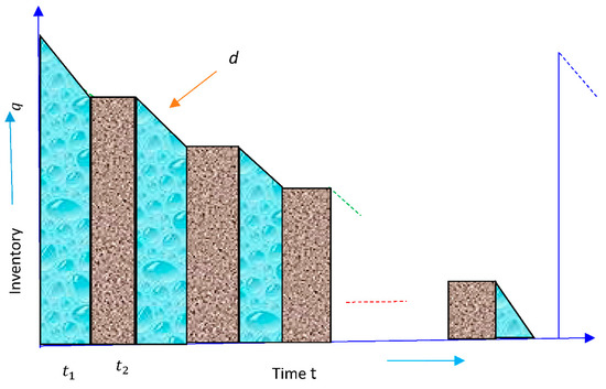
Figure 3.
Logistic diagram of inventory system.
The inventory holding cost (HC) can be obtained as
where
and
idle time cost
and the cycle time
Now, using Equations (3)–(7), the total average profit per cycle is given by
Now our problem is given by
Subject to the conditions (4), (5), and (7).
Now problem (9) can be written as
Subject to the conditions (4), (5), and (7)
where
Please note that, if then so Equation (8) reduces to
this is the case of classical EOQ model.
4. Fuzzy Mathematical Model
In many practical problems, several parameters associated in the model assume flexible values. Therefore, the demand rate, the several cost components, and both of them may assume fuzzy numbers. Consequently, the fuzzy model splits into three different models namely Model 1, Model 2 and Model 3, respectively, and they are stated as follows.
4.1. Model 1: When Demand Rate Assumes Dense Fuzzy Number
Since the demand rate assumes flexibility in nature throughout an inventory process. Therefore, the objective function of the crisp model (10) can be reduced to
where and are given by (11).
Again, (10) can also be rewritten as
The membership function of the demand rate having m learning frequency of dense fuzzy set is given by
Now, the left and the right cuts of are given by
However, utilizing (14) in (15) the membership functions of the fuzzy objective become
where the left and right cuts of are given by
Thus, as per Reference [23] the index value of the fuzzy objective is
where M is the total number of turnovers (learning frequency) to achieve the maturity in learning experiences. Now, if the demand rate assumes triangular dense fuzzy lock set then its membership function will be
The left and right cuts of the are
The corresponding index value is given by
Again utilizing (14) in (19) the membership function of the fuzzy objective becomes
Now the left and right cuts of are given by
The corresponding index value is
Special Cases
- (i)
- If in (22) then
- (ii)
- If in (i) then , the case of single key
- (iii)
- If in (ii) then , the case of general fuzzy number.
- (iv)
- If in (iii) then , the case of crisp model.
Discussion on various fuzzy models
- (i)
- Problem of Dense fuzzy modelReferring (11), (16), and (18) the problem can be formulated as
- (ii)
- Problem of Dense fuzzy lock modelReferring to (19) and (22), the problem can be formulated asand the other parameters obtained in (23). Please note that for single key .
- (iii)
- Problem of general fuzzy modelTo set up the model considering then (24) becomesand the other parameters taken from (23).
Corollary 1.
Rules of finding key values of the fuzzy locks
For every fuzzy parameter there exists two bounds namely a upper limit (if known), lower limit (if known) or both. For single key, if upper bound is available then the index value ofis given byimplies. If the lower bound is known, thenimplies. For double keys the index value ofis given by,Therefore,and.
Numerical Example 1
Considering the data set studied by De and Sana [23] and let . Here the bounds of demand rate assume as . Employing the above definition, the key values for the demand rate are obtained as
Satisfying the above condition let and then the optimal solution of the several models can be put in Table 1.

Table 1.
Optimal solution of the economic order quantity (EOQ) model.
4.2. Model 2: When the Cost/Price Components Assume Fuzzy Number
Now in this section, considering the cost/price components as TDFLS to study whether it gives better results than that of demand rate for TDFLS or not. Before applying TDFLS rule the original crisp problem (9) can be reduced to
where
Now, if the cost vector takes a triangular dense fuzzy lock set then the corresponding average inventory profit becomes
where for .
Therefore, as per De [34], the index value of the fuzzy objective is given by
Thus, the crisp equivalent problem of the fuzzy objective (28) is
Particular cases
- (i)
- If then gives the crisp problem.
- (ii)
- If for thengives the general fuzzy problem.
- (iii)
- If for thengives the problem of dense fuzzy model.
- (iv)
- If for thengives the problem of dense fuzzy lock model for single key.
- (v)
- If for thengives the problem of dense fuzzy lock model for double keys.
Corollary 2.
Method of finding the keys of the fuzzy lock sets of cost vectors
As per De [34], the keys of fuzzy cost vectors can be obtained from for as which is coming from the left and right α-cuts that splits into and respectively. Let the lower and upper bounds of each cost parameters are and respectively. Thus, it is clear that and giving and for double keys and that for single key
Numerical Example 2
Considering the data set studied by De and Sana [23] and let Here the bounds of the different cost vectors assumes as follows: and . Employing Corollary 2 the various key vectors are obtained as follows
And that for single key it becomes,
Now for practical purpose consider for single key and that for double keys which must satisfy the above constraints. Thus, the optimum average inventory profit is found in Table 2.
Table 2.
Optimum solution for EOQ model under cost/price fuzzy Locks.
4.3. Model 3: When Demand Rate and Cost/Price All Assume to Be Fuzzy Numbers
In this section, considering the demand rate and costs/prices all parameters as TDFLS to check whether this gives finer optimum than Model 1 and Model 2 or not. First of all Equation (9) can be simplified as follows.
where
Now, let the cost vector and demand rate both orient with a triangular dense fuzzy lock set and the corresponding average inventory profit is reduces to
With for and . Therefore, as per De [34], the index value of the fuzzy objective is given by
Thus, the crisp equivalent problem of the fuzzy objective (36) is
Particular cases
- (i)
- If then gives the crisp problem.
- (ii)
- If for thengives the general fuzzy problem.
- (iii)
- If for thengives the problem of dense fuzzy model.
- (iv)
- If for thengives the problem of dense fuzzy lock model for single key.
- (v)
- If for thengives the problem of dense fuzzy lock model for double keys.
Numerical Example 3
Let the parameters assume the values which are used in the numerical Examples 1 and 2. Thus, solving (38), and the optimal result is obtained in Table 3.
Table 3.
Optimum solution for Model 3.
4.4. Discussion on Numerical Results Obtained in Model 1, Model 2, and Model 3
From optimum solution Table 1, the case of Model 1 (when only demand rate assumes fuzzy) it is seen that the optimality exists at four learning frequencies for three days cycle times of 12.12 h of opening time per day under several methodological environments. However, in crisp environments, the profit value was $16,759.89 viz. it began to enhance to $18,194.72 for the double keys of lock fuzzy environments. Table 2 (when only cost parameters assume fuzzy) reveals that the optimum profit value keeps $17,505.34 in general fuzzy environment viz. in dense fuzzy environment it gets the value $17,186.75 and finally the profit function reaches to $19,681.38 for double key of lock fuzzy environment. In Table 3 of Model 3 (when all parameters assume fuzzy) it was observed that for the same learning frequency and the same cycle time as obtained in the earlier cases, the profit function was the highest value under general fuzzy ($18,161.8), dense fuzzy ($17,705.93), lock fuzzy with single key ($19,519.68), and that for double key ($21,216.8) environment, respectively, with respect to the other models. Therefore, Model 3 gives the ultimate maximum value for the average profit function among other models.
4.5. Sensitivity Analysis
Since Model 3 gives over all optimum so the sensitivity analysis has been made for the double key parameters of the cost vector and demand rate also which are associated in the EOQ model. Considering the parametric changes from −50% to +50% for each of the keys taking one at a time and keeping others as constants the optimum result is obtained in Table 4.
Table 4.
Sensitivity analysis for Model 3.
Table 4 shows that whatever be the changes of demand rate and cost vectors within −50% to +50% of any keys, the profit function is ultimately increasing to a considerable average profit from 23.02% to 37.28% as well. It was also seen that the order quantity gets fixed value 81.22 units for the change of the key vectors of the several cost components. Although the order quantity gets a range of variation from 79.09 units to 87.59 units for the change of demand rate alone. However, it was observed that the optimum cycle time be 3 days (= n + 1) in all the cases with respect to the learning frequency 4.
4.6. Solution Procedure for Dense Fuzzy Lock Set Model
To get the optimum value of the objective function of the proposed model, a computer-based algorithm and flow chart can be included in the following manner.
Solution Algorithm and Flow Chart over Dense Fuzzy Lock Set Model
The solution algorithm is stated as follows:
- Input .
- Find average profit (Crisp) using Equations (4), (5), (7), and (9).
- Apply general fuzzy (a) when d is fuzzy (b) when and d are fuzzy and (c) when are fuzzy only.
- Find corresponding average profit using Equations (25), (30), and (39), respectively.
- Find
- Check if yes go to step 7 else go to step 8.
- Set go to step 9.
- Set
- Apply dense fuzzy rule over the parameters.
- Consider three cases d is dense fuzzy, and d are dense fuzzy, are dense fuzzy.
- Find corresponding average profit respectively using Equations (23), (39), and (31).
- Find corresponding average profit .
- Check if yes go to step 14 else go to step 15.
- Set
- Apply fuzzy lock set of single key over the fuzzy parameters.
- Consider three cases d is fuzzy lock, and d are fuzzy lock, are fuzzy lock.
- Find corresponding average profit using Equations (24), (32), and (41), respectively.
- Find
- Check if yes go to step 20 else go to step 21.
- Set
- Apply fuzzy lock set of double keys over the fuzzy parameters.
- Consider three cases d is fuzzy lock, and d are fuzzy lock, are fuzzy lock.
- Find corresponding average profit using Equations (24), (33) and (42) respectively
- Find
- Check if yes go to step 26 else go to step 27.
- is optimum, go to step 25.
- is optimum.
- End.
The flow chart of the above algorithm can be developed as Figure 4:
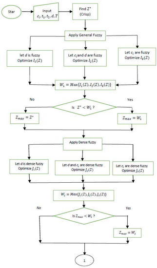
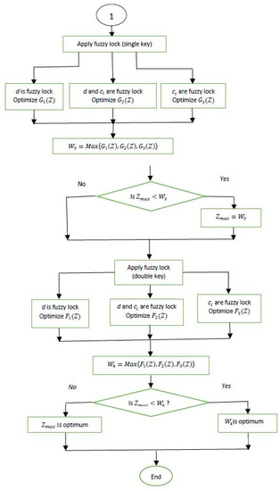
Figure 4.
Flow chart of the proposed mode.
Remark 3.
Based on proposed algorithm the flow chart has been drawn. From the input data the crisp problem has been solved first. After that, general fuzzy methodology has been employed on demand, cost parameters, and both demand and cost parameters separately; take maximum value (since it is a profit function) after optimizing them and compare this value with crisp optimum to get maximum among them. Then dense fuzzy methodology has been applied in a similar way to get optimum value among them. Thereafter dense fuzzy with single key and finally dense fuzzy with double key have been utilized to get finer optimum. After applying all fuzzy environments in the proposed model, all maximum values have been ordered to get final profit value.
4.7. Graphical Illustration
Several graphs have been drawn utilizing the data (Table 1, Table 2, Table 3 and Table 4). A comparative discussion over Model 1, Model 2 and Model 3 (shown in Figure 4) has been done using the data set of Table 1, Table 2 and Table 3. Figure 5 has been drawn using the data of the sensitivity analysis (Table 4).
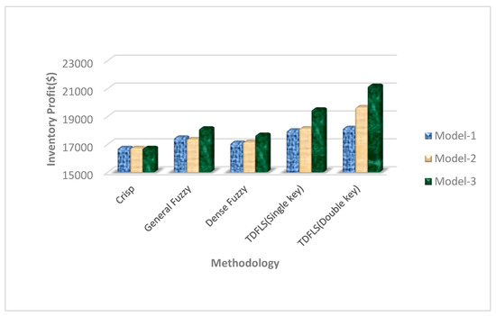
Figure 5.
Comparison between Model 1, Model 2 and Model 3.
Figure 5 shows the average inventory profit assumes minimum value for crisp sense and that gets maximum value for dense fuzzy lock of double keys environment throughout the Model 1, Model 2 and Model 3 exclusively. This study also reveals that general fuzzy environment gives supremum average profit value than that of dense fuzzy environment. However, the dense fuzzy lock environment of single key always corresponds to the finer average profit function than all other cases except the cases of fuzzy lock of double keys.
Figure 6 shows that the average profit value of Model 3 gets almost insensitive when unit selling price and idle time cost get values from −50% to +50% separately. Moreover, the profit value assumes remarkable variation when the holding cost, set up cost, and demand rate changes from −50% to +50% separately. Thus, the basic managerial insight is to have more profit and the parameters like unit holding cost, set up cost, and demand rate of the inventory process might decrease up to 50% all the time.
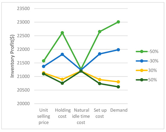
Figure 6.
Graphical illustration of sensitivity analysis.
5. Conclusions
Natural idle time is an emergent situation in any kind of inventory management problem. This idle time can be considered by means of usual closing time duration per day. Also due to the huge pressures of population in each and every country in the world, the market itself creates large demands for essential commodities which are used in daily life. However, the capacity of production as well as natural resources and the capital involved to run the inventory process are also limited to some extent. Therefore, it is natural that any one commodity may not be available whenever it is demanded. In such cases, the exact decision can be made with the help of controlling the key vector of the corresponding fuzzy locks. Such kind of behavior representing the counterpart of the learning experiences of the management process which are genuinely modern trends of any enterprises of inventory management. Thus, the basic novelties of this article are:
- (a)
- Inventory problems should be optimized with the help of dense fuzzy lock set rules instead of dense fuzzy rules.
- (b)
- Double key vectors may be able to maximize the average profit function instead of taking single key vectors for managerial decision-making.
- (c)
- Optimum results can be checked and updated through a computer-based algorithm.
Author Contributions
All authors equally contributed in each section.
Funding
This research received no external funding.
Acknowledgments
The authors are thankful to the anonymous reviewers for their valuable comments and suggestions to improve the quality of the present article.
Conflicts of Interest
The authors declare no conflict of interest.
Appendix A
Defining several costs associated in the proposed model.
1. Set-up cost(b):
The cost of setting a production plant/inventory is called setup cost. It includes costs of developing infrastructure, requisition, follow-up, receiving the goods, quantity control, etc. These are also called order costs or replenishment costs per production run (cycle). They are assumed to be independent of the quantity ordered or produced.
2. Unit selling price (p):
It is the price which can be obtained after the sale of one unit of item. This includes the price which gets value after deduction (if any) on marked (announced or declared) price value on the corresponding items.
3. Average natural idle time cost per unit idle time (ic):
In a broad sense, this is the per-hour cost of the maintenance of the inventory process at the closing period of the process. The natural closing period is generally viewed as “natural idle time” of the process. For instance, 9 p.m. to 9 a.m. is the non-shopping/marketing/business time in a day. This includes per hour cost of telephone calls, security charges, electricity bills, etc.
4. Holding cost():
The cost to carry or hold the goods in stock is known as holding or carrying cost per unit of goods for a unit of time. Holding cost is assumed to vary directly with the size of inventory as well as the time for which the item is held in stock. The following components constitute the holding cost:
- (i)
- Invested capital cost.
- (ii)
- Record-keeping and administrative cost.
- (iii)
- Handling cost.
- (iv)
- Storage cost.
- (v)
- Taxes and insurance costs.
References
- Nash, J.F. The bargaining problem. Econometrica 1950, 18, 155–162. [Google Scholar] [CrossRef]
- Zadeh, L.A. Fuzzy sets. Inf. Control 1965, 8, 338–356. [Google Scholar] [CrossRef]
- Bellman, R.E.; Zadeh, L.A. Decision making in a fuzzy environment. Manag. Sci. 1970, 17, 141–164. [Google Scholar] [CrossRef]
- Dubois, D.; Prade, H. Operations on fuzzy numbers. Int. J. Syst. Sci. 1978, 9, 613–626. [Google Scholar] [CrossRef]
- Kaufmann, A.; Gupta, M.M. Introduction of Fuzzy Arithmetic Theory and Applications; Van Nostrand Reinhold: New York, NY, USA, 1985. [Google Scholar]
- Baez-Sancheza, A.D.; Morettib, A.C.; Rojas-Medarc, M.A. On polygonal fuzzy sets and numbers. Fuzzy Sets Syst. 2012, 209, 54–65. [Google Scholar] [CrossRef]
- Beg, I.; Ashraf, S. Fuzzy relational calculus. Bull. Malaysian Math. Sci. Soc. 2014, 37, 203–237. [Google Scholar]
- Deli, I.; Broumi, S. Neutrosophic soft matrices and NSM-decision making. J. Intell. Fuzzy Syst. 2015, 28, 2233–2241. [Google Scholar] [CrossRef]
- Kumar, R.S. Modelling a type-2 fuzzy inventory system considering items with imperfect quality ad shortage backlogging. Sadhana 2018, 43, 163–175. [Google Scholar] [CrossRef]
- Diamond, P. The Structure of Type k Fuzzy Numbers, in the Coming of Age of Fuzzy Logic; Bezdek, J.C., Ed.; World Scientific Publishing: Seattle, WA, USA, 1989; pp. 671–674. [Google Scholar]
- Diamond, P. A note on fuzzy star shaped fuzzy sets. Fuzzy Sets Syst. 1990, 37, 193–199. [Google Scholar] [CrossRef]
- Chutia, R.; Mahanta, S.; Baruah, H.K. An alternative method of finding the membership of a fuzzy number. Int. J. Latest Trends Comput. 2010, 1, 69–72. [Google Scholar]
- Roychoudhury, S.; Pedrycz, W. An alternative characterization of fuzzy complement functional. Soft Comput.—Fusion Found. Methodol. Appl. 2003, 7, 563–565. [Google Scholar] [CrossRef]
- Bobeylev, V.N. Cauchy problem under fuzzy control. BUSEFAL 1985, 21, 117–126. [Google Scholar]
- Bobeylev, V.N. On the reduction of fuzzy number to real. BUSEFAL 1988, 35, 100–104. [Google Scholar]
- Buckley, J.J. Generalized and extended fuzzy sets with applications. Fuzzy Sets Syst. 1988, 25, 159–174. [Google Scholar] [CrossRef]
- Roy, A.R.; Maji, P.K. A fuzzy soft theoretic approach to decision making problems. J. Comput. Appl. Math. 2010, 203, 412–418. [Google Scholar] [CrossRef]
- Molodtsov, D. Soft set theory first result. Comput. Math. Appl. 1999, 37, 19–31. [Google Scholar] [CrossRef]
- Cagman, N.; Enginoglu, S.; Citak, F. Fuzzy soft theory and its application. Int. J. Fuzzy Syst. 2011, 8, 137–147. [Google Scholar]
- Pawlak, Z. Rough sets. Int. J. Inf. Comput. Sci. 1982, 11, 341–356. [Google Scholar] [CrossRef]
- Torra, V. Hesitant fuzzy sets. Int. J. Intell. Syst. 2010, 25, 529–539. [Google Scholar] [CrossRef]
- Karmakar, S.; De, S.K.; Goswami, A. A deteriorating EOQ model for natural idle time and imprecise demand: Hesitant fuzzy approach. Int. J. Syst. Sci. Oper. Logist. 2015. [Google Scholar] [CrossRef]
- De, S.K.; Sana, S.S. Multi-criterion multi-attribute decision-making for an EOQ model in a hesitant fuzzy environment. Nat. Sci. Eng. 2015, 17, 61–68. [Google Scholar]
- De, S.K.; Beg, I. Triangular dense fuzzy sets and new defuzzification methods. J. Intell. Fuzzy Syst. 2016, 31, 469–477. [Google Scholar] [CrossRef]
- De, S.K.; Beg, I. Triangular dense fuzzy Neutrosophic sets. Neutrosophic Sets Syst. 2016, 13, 24–37. [Google Scholar]
- De, S.K.; Mahata, G.C. Decision of a fuzzy inventory with fuzzy backorder model under cloudy fuzzy demand rate. Int. J. Appl. Comput. Math. 2016. [Google Scholar] [CrossRef]
- Karmakar, S.; De, S.K.; Goswami, A. A pollution sensitive remanufacturing model with waste items: Triangular dense fuzzy lock set approach. J. Clean. Prod. 2018. [Google Scholar] [CrossRef]
- Karmakar, S.; De, S.K.; Goswami, A. A pollution sensitive dense fuzzy economic production quantity model with cycle time dependent production rate. J. Clean. Prod. 2017. [Google Scholar] [CrossRef]
- Maity, S.; De, S.K.; Pal, M. Two decision makers’ single decision over a back order EOQ model with dense fuzzy demand rate. J. Financ. Mark. 2018, 3. [Google Scholar] [CrossRef]
- Boccia, M.; Crainic, T.G.; Sforza, A.; Sterle, C. Multi-commodity location-routing: Flow intercepting formulation and branch-and-cut algorithm. Comput. Oper. Res. 2018, 89, 94–112. [Google Scholar] [CrossRef]
- Charkhgarda, H.; Savelsbergh, M.; Talebian, M. A linear programming-based algorithm to solve a class of optimization problems with a multi-linear objective function and affine constraints. Comput. Oper. Res. 2018, 89, 17–30. [Google Scholar] [CrossRef]
- Nash, J.F.; Shao, L.; Ehrgott, M. Primal and dual multi-objective linear programming algorithms for linear multiplicative programmes. Optimization 2016, 65, 415–431. [Google Scholar]
- Pelt, T.D.; Fransoo, J.C. A note on “Linear programming models for a stochastic dynamic capacitated lot sizing problem”. Comput. Oper. Res. 2018, 89, 13–16. [Google Scholar] [CrossRef]
- De, S.K. Triangular dense fuzzy lock set. Soft Comput. 2017. [Google Scholar] [CrossRef]
© 2019 by the authors. Licensee MDPI, Basel, Switzerland. This article is an open access article distributed under the terms and conditions of the Creative Commons Attribution (CC BY) license (http://creativecommons.org/licenses/by/4.0/).