Imperfect Multi-Stage Lean Manufacturing System with Rework under Fuzzy Demand


Abstract
1. Introduction
2. Materials and Methods
2.1. Assumptions
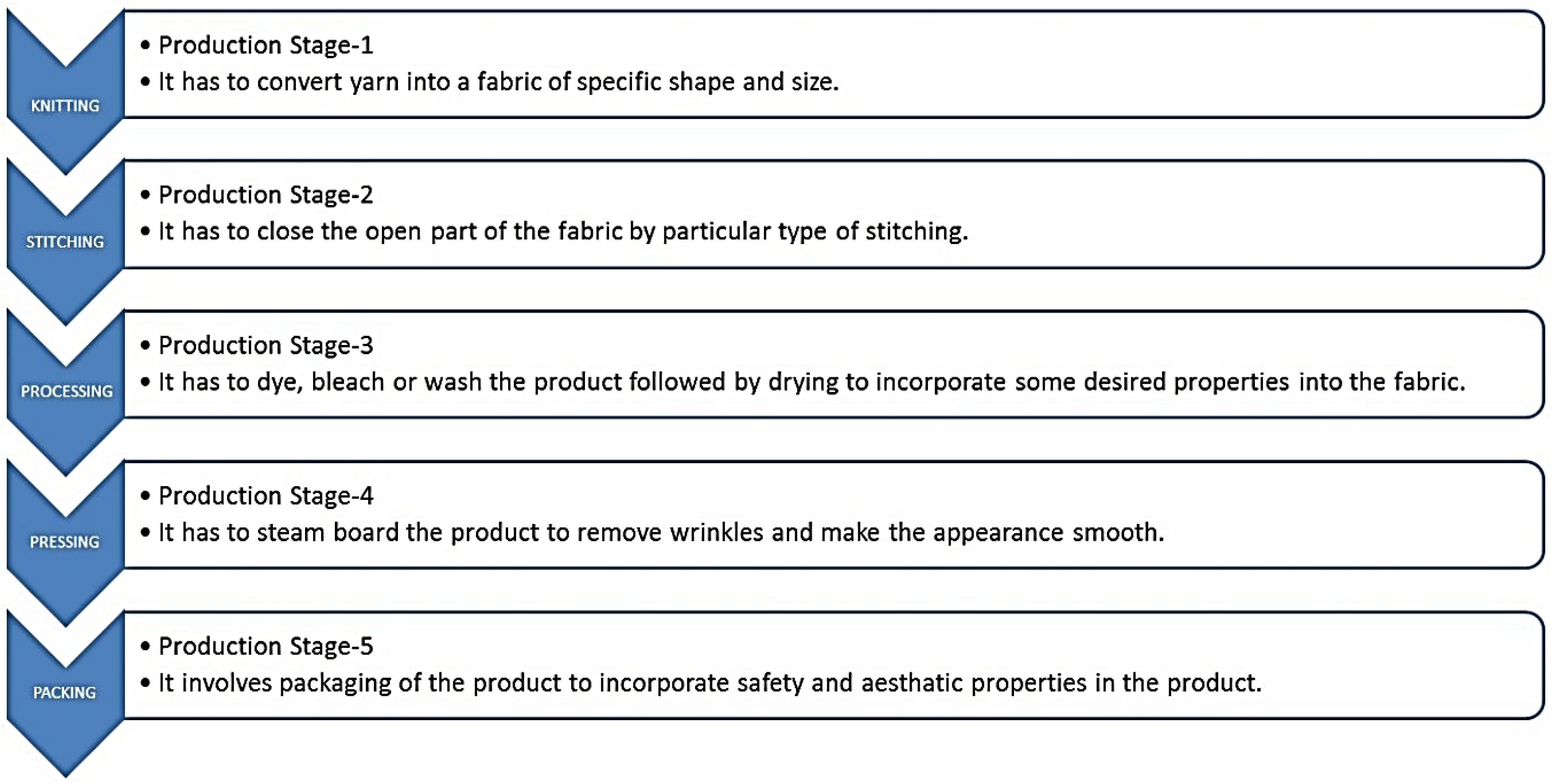
- A single type of item is produced in an n-stage production system.
- Production runs are fairly consistent, i.e., system is assumed to be a lean manufacturing system where inventory behavior follows a similar trend in repetitive production cycles.
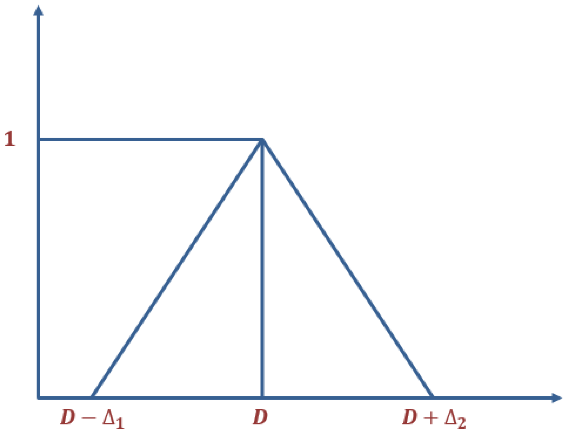
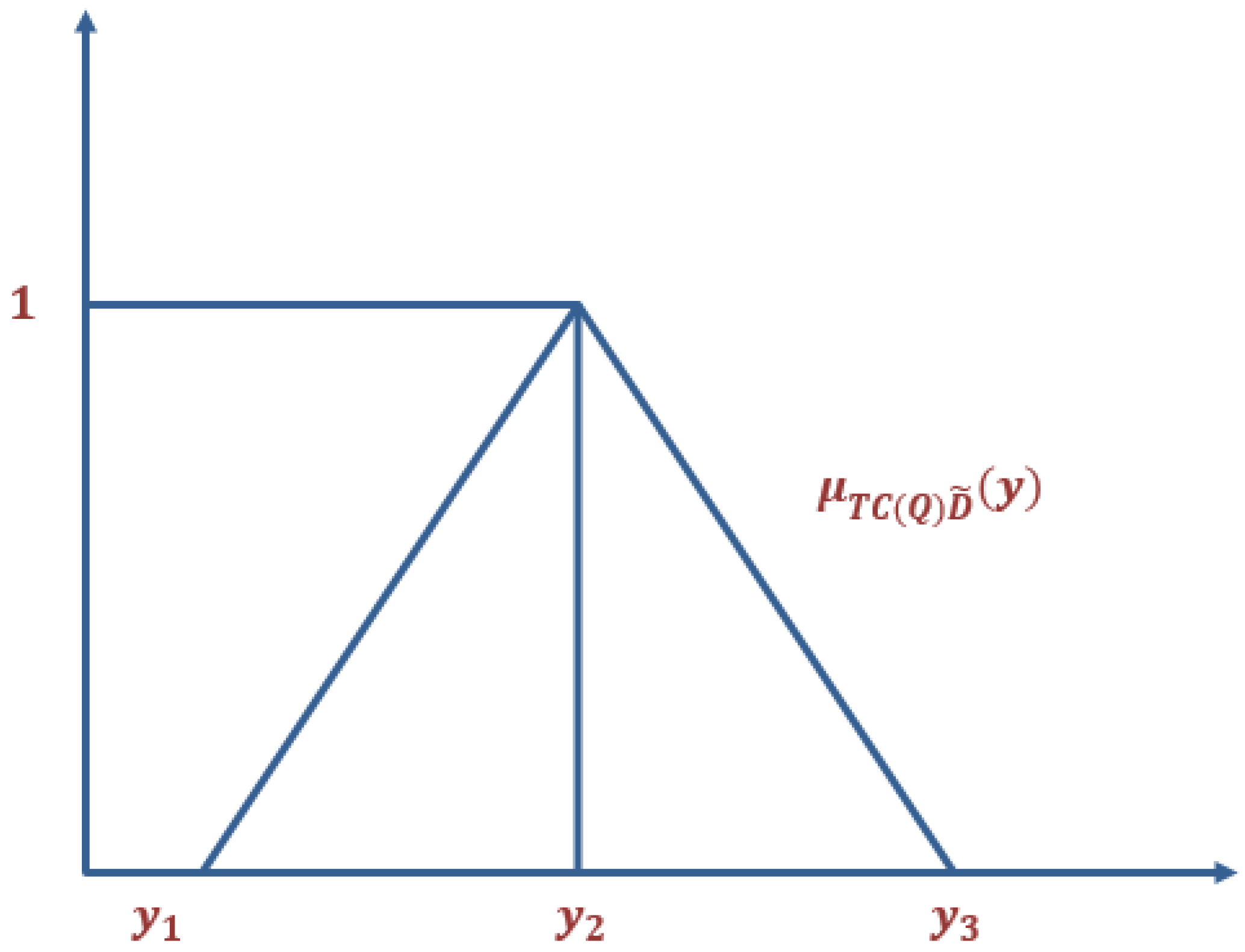
- Uncertain product demand is measured as a Triangular Fuzzy Number (TFN).
- Inline inspections provides effective results, determines the defective items immediately, and helps the managers to make immediate decisions over it. This model assumes that defective items are detected during the hundred percent inline inspection.
- In textile industries, defective items are generally reworked. This model assumes reworking of defective items at each production stage. The reworking process is considered as perfect and no item is scrapped.
- Defective rate is constant at each production stage, but it may vary from stage to stage.
- Setup time of each production stage is percent of the total time of that production stage.
- Transportation time and cost among the production stages is assumed to be negligible.
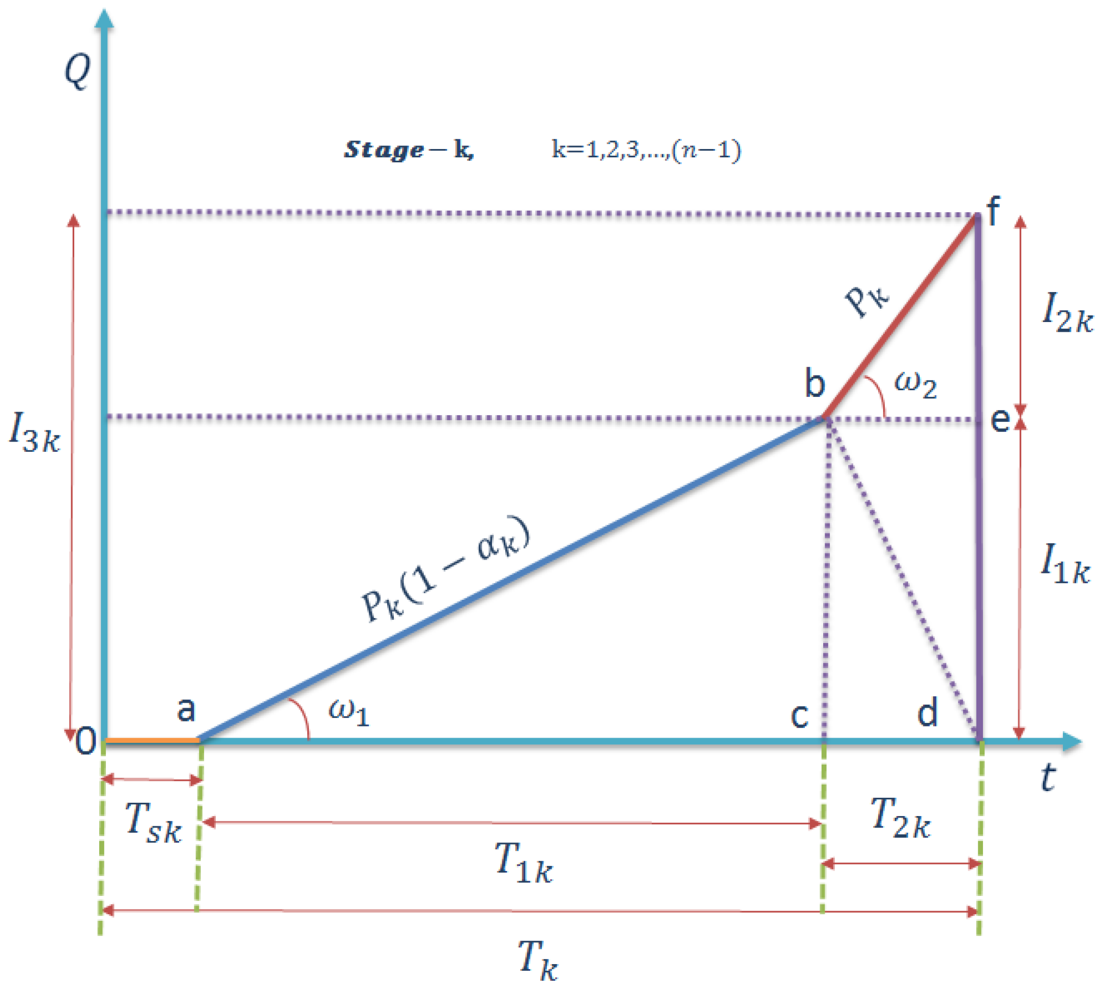
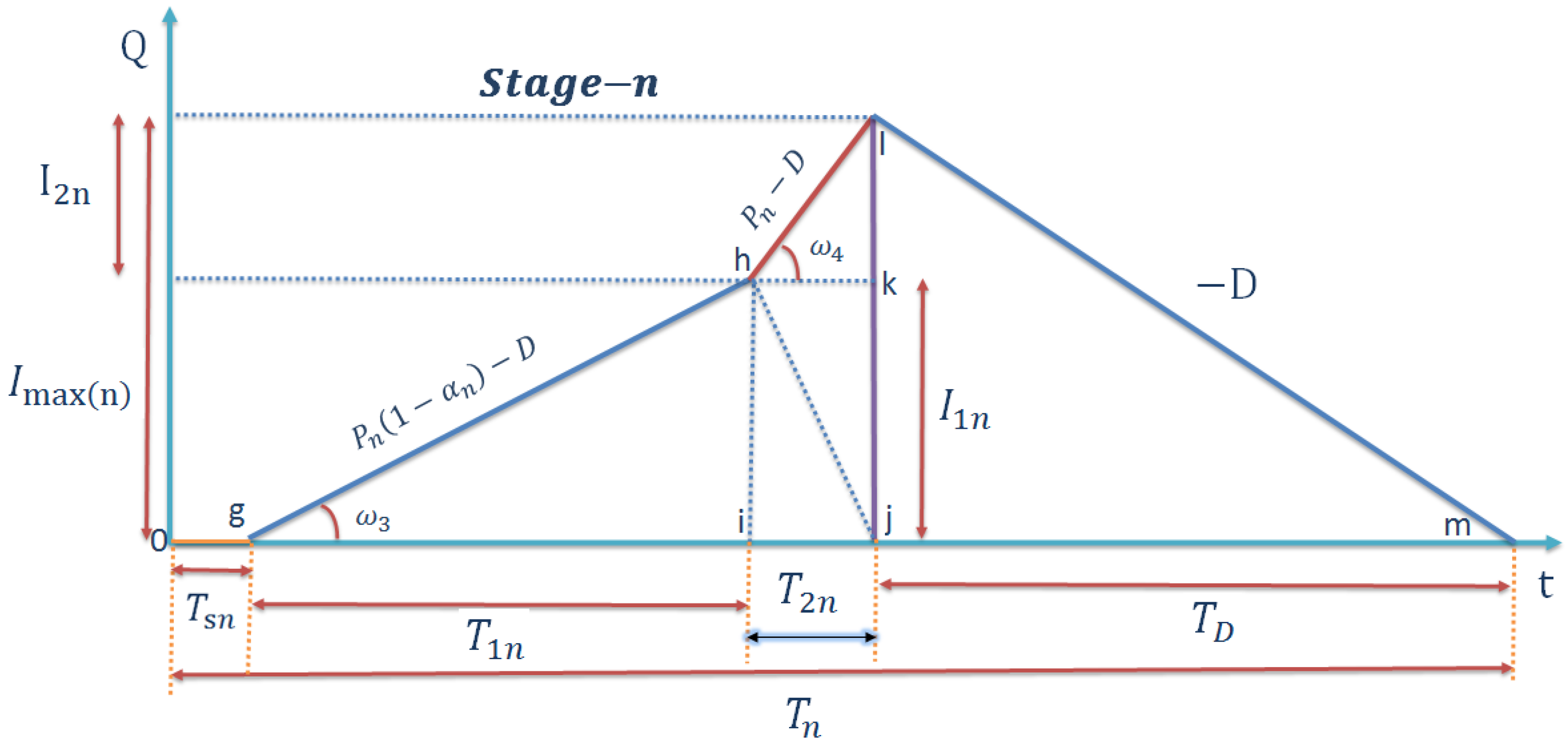
2.2. Model Formulation
3. Numerical Experiment and Results
3.1. Example 1
3.2. Example 2
3.3. Example 3
4. Discussion
- It is evident from the change in optimal cost function that the order processing cost () is the most sensitive factor than other parameters. One can observe that with each percentage increase in there exists almost similar amount of percentage increase in the system cost. For instance, regarding four-stage production system in Example 2, system cost increases by 24.17% by the increment of 25% in order of processing cost, and 48.34% increase in system cost is observed by a 50% rise in the order of processing cost.
- Next to the effect of order processing cost is the impact of production rate () on the system cost. It can be noted that the effect of production rate on the production system with higher number of stages is more than the system with a lower number of production stages. This illustrates the necessity of wisely adjusting production rate at each production stage to keep the system cost at its minimum value.
- An interesting observation from the sensitivity analysis of all the numerical examples reveal that the impact of setup cost () and the inventory holding cost () is same on the system cost for all the production systems with any number of stages. Thus, the decision makers have to make intelligent decision in putting efforts to reduce one of these costs first. Here arises the importance of lean philosophy, as Single Minute Exchange of Dyes (SMED) is the best possible solution for setup cost reduction. Therefore, managers should make efforts to apply SMED for setup cost reduction first, as it is much more beneficial than cutting down stock management equipment and inventory holding staff.
- Inspection cost () and defective proportion () bear trivial impact on the system cost that gradually varies as the system moves towards a higher number of stages.
5. Conclusions
Author Contributions
Funding
Conflicts of Interest
Nomenclature
| Indices | |
| k | production stages (k = 1, 2, 3… (n − 1)) |
| i | production stages (i = 1, 2, 3… n) |
| Decision variable | |
| Q | lot size (items) |
| Parameters | |
| number of production stages | |
| production rate for production stage (items per unit time) | |
| production rate for production stage (items per unit time, where ) | |
| demand rate (fuzzy, and fulfilled at production stage) | |
| defective proportion at production stage | |
| defective proportion at production stage | |
| cycle time of production stage (years) | |
| cycle time of production stage (years) | |
| time between production runs (total cycle time of -stages, years) | |
| setup cost of production stage ($/setup) | |
| inventory holding cost of finished items ($/item/year) | |
| order processing cost at production stage ($/item/stage) | |
| inspection cost at production stage ($/item/stage) | |
| percentage setup time per stage | |
| average inventory of finished items in the system | |
| total cost of the production system ($ per unit time) | |
Abbreviations
| EOQ | Economic order quantity |
| EPQ | Economic production quantity |
| TFN | Triangular fuzzy number |
| FMF | Fuzzy membership function |
| SMED | Single minute exchange of dyes |
References
- Hodge, G.L.; Goforth Ross, K.; Joines, J.A.; Thoney, K. Adapting lean manufacturing principles to the textile industry. Prod. Plan. Control 2011, 22, 237–247. [Google Scholar] [CrossRef]
- Harris, F.W. How many parts to make at once. Fact. Mag. Manag. 1913, 10, 135–136. [Google Scholar] [CrossRef]
- Taft, E.W. The most economical production lot. Iron Age 1918, 101, 1410–1412. [Google Scholar]
- Lee, H.L. Lot sizing to reduce capacity utilization in a production process with defective items, process corrections, and rework. Manag. Sci. 1992, 38, 1314–1328. [Google Scholar] [CrossRef]
- Gupta, T.; Chakraborty, S. Looping in a multistage production system. Int. J. Prod. Res. 1984, 22, 299–311. [Google Scholar] [CrossRef]
- Tayi, G.K.; Ballou, D.P. An integrated production-inventory model with reprocessing and inspection. Int. J. Prod. Res. 1988, 26, 1299–1315. [Google Scholar] [CrossRef]
- Lee, H.H.; Chandra, M.J.; Deleveaux, V.J. Optimal batch size and investment in multistage production systems with scrap. Prod. Plan. Control 1997, 8, 586–596. [Google Scholar] [CrossRef]
- Glock, C.H.; Jaber, M.Y. Learning effects and the phenomenon of moving bottlenecks in a two-stage production system. Appl. Math. Model. 2013, 37, 8617–8628. [Google Scholar] [CrossRef]
- Lin, C.S. Integrated production-inventory models with imperfect production processes and a limited capacity for raw materials. Math. Comput. Model. 1999, 29, 81–89. [Google Scholar] [CrossRef]
- Salameh, M.K.; Jaber, M.Y. Economic production quantity model for items with imperfect quality. Int. J. Prod. Econ. 2000, 64, 59–64. [Google Scholar] [CrossRef]
- Khan, M.; Jaber, M.Y.; Guiffrida, A.L.; Zolfaghari, S. A review of the extensions of a modified EOQ model for imperfect quality items. Int. J. Prod. Econ. 2011, 132, 1–2. [Google Scholar] [CrossRef]
- Jaber, M.Y.; Zanoni, S.; Zavanella, L.E. Economic order quantity models for imperfect items with buy and repair options. Int. J. Prod. Econ. 2014, 155, 126–131. [Google Scholar] [CrossRef]
- Ouyang, L.Y.; Chen, C.K.; Chang, H.C. Quality improvement, setup cost and lead-time reductions in lot size reorder point models with an imperfect production process. Comput. Oper. Res. 2002, 29, 1701–1717. [Google Scholar] [CrossRef]
- Cárdenas-Barrón, L.E. Economic production quantity with rework process at a single-stage manufacturing system with planned backorders. Comput. Ind. Eng. 2009, 57, 1105–1113. [Google Scholar] [CrossRef]
- Eroglu, A.; Ozdemir, G. An economic order quantity model with defective items and shortages. Int. J. Prod. Econ. 2007, 106, 544–549. [Google Scholar] [CrossRef]
- Jaber, M.Y.; Guiffrida, A.L. Learning curves for imperfect production processes with reworks and process restoration interruptions. Eur. J. Oper. Res. 2008, 189, 93–104. [Google Scholar] [CrossRef]
- Ben-Daya, M. The economic production lot-sizing problem with imperfect production processes and imperfect maintenance. Int. J. Prod. Econ. 2002, 76, 257–264. [Google Scholar] [CrossRef]
- Jamal, A.M.; Sarker, B.R.; Mondal, S. Optimal manufacturing batch size with rework process at a single-stage production system. Comput. Ind. Eng. 2004, 47, 77–89. [Google Scholar] [CrossRef]
- Biswas, P.; Sarker, B.R. Optimal batch quantity models for a lean production system with in-cycle rework and scrap. Int. J. Prod. Res. 2008, 46, 6585–6610. [Google Scholar] [CrossRef]
- Chung, K.J. The economic production quantity with rework process in supply chain management. Comput. Math. Appl. 2011, 62, 2547–2550. [Google Scholar] [CrossRef]
- Taleizadeh, A.A.; Jalali-Naini, S.G.; Wee, H.M.; Kuo, T.C. An imperfect multi-product production system with rework. Sci. Iran 2013, 20, 811–823. [Google Scholar]
- Cárdenas-Barrón, L.E. Optimal manufacturing batch size with rework in a single-stage production system—A simple derivation. Comput. Ind. Eng. 2008, 55, 758–765. [Google Scholar] [CrossRef]
- Ma, W.N.; Gong, D.C.; Lin, G.C. An optimal common production cycle time for imperfect production processes with scrap. Math. Comput. Model. 2010, 52, 724–737. [Google Scholar] [CrossRef]
- Barzoki, M.R.; Jahanbazi, M.; Bijari, M. Effects of imperfect products on lot sizing with work in process inventory. Appl. Math. Comput. 2011, 217, 8328–8336. [Google Scholar] [CrossRef]
- Chiu, S.W.; Tseng, C.T.; Wu, M.F.; Sung, P.C. Multi-item EPQ model with scrap, rework and multi-delivery using common cycle policy. J. Appl. Res. Technol. 2014, 12, 615–622. [Google Scholar] [CrossRef]
- Chiu, S.W.; Chiu, Y.S.; Yang, J.C. Combining an alternative multi-delivery policy into economic production lot size problem with partial rework. Expert Syst. Appl. 2012, 39, 2578–2583. [Google Scholar] [CrossRef]
- Noorollahi, E.; Karimi-Nasab, M.; Aryanezhad, M.B. An economic production quantity model with random yield subject to process compressibility. Math. Comput. Model. 2012, 56, 80–96. [Google Scholar] [CrossRef]
- Moussawi-Haidar, L.; Salameh, M.; Nasr, W. Production lot sizing with quality screening and rework. Appl. Math. Model. 2016, 40, 3242–3256. [Google Scholar] [CrossRef]
- Chiu, S.W.; Gong, D.C.; Wee, H.M. Effects of random defective rate and imperfect rework process on economic production quantity model. Jpn. J. Ind. Appl. Math. 2004, 21, 375. [Google Scholar] [CrossRef]
- Taleizadeh, A.A.; Cárdenas-Barrón, L.E.; Mohammadi, B. A deterministic multi product single machine EPQ model with backordering, scraped products, rework and interruption in manufacturing process. Int. J. Prod. Econ. 2014, 150, 9–27. [Google Scholar] [CrossRef]
- Chiu, S.W.; Ting, C.K.; Chiu, Y.S. Optimal production lot sizing with rework, scrap rate, and service level constraint. Math. Comput. Model. 2007, 46, 535–549. [Google Scholar] [CrossRef]
- Taleizadeh, A.A.; Wee, H.M.; Jalali-Naini, S.G. Economic production quantity model with repair failure and limited capacity. Appl. Math. Model. 2013, 37, 2765–2774. [Google Scholar] [CrossRef]
- Sana, S.S. A production–inventory model in an imperfect production process. Eur. J. Oper. Res. 2010, 200, 451–464. [Google Scholar] [CrossRef]
- Sarkar, B.; Moon, I. An EPQ model with inflation in an imperfect production system. Appl. Math. Comput. 2011, 217, 6159–6167. [Google Scholar] [CrossRef]
- Yoo, S.H.; Kim, D.; Park, M.S. Lot sizing and quality investment with quality cost analyses for imperfect production and inspection processes with commercial return. Int. J. Prod. Econ. 2012, 140, 922–933. [Google Scholar] [CrossRef]
- Chakraborty, T.; Giri, B.C. Joint determination of optimal safety stocks and production policy for an imperfect production system. Appl. Math. Model. 2012, 36, 712–722. [Google Scholar] [CrossRef]
- Wee, H.M.; Wang, W.T.; Yang, P.C. A production quantity model for imperfect quality items with shortage and screening constraint. Int. J. Prod. Res. 2013, 51, 1869–1884. [Google Scholar] [CrossRef]
- Chiu, S.W.; Chou, C.L.; Wu, W.K. Optimizing replenishment policy in an EPQ-based inventory model with nonconforming items and breakdown. Econ. Model. 2013, 35, 330–337. [Google Scholar] [CrossRef]
- Sarkar, B.; Cárdenas-Barrón, L.E.; Sarkar, M.; Singgih, M.L. An economic production quantity model with random defective rate, rework process and backorders for a single stage production system. J. Manuf. Syst. 2014, 33, 423–435. [Google Scholar] [CrossRef]
- Dang, J.F.; Hong, I.H. The Cournot game under a fuzzy decision environment. Comput. Math. Appl. 2010, 59, 3099–3109. [Google Scholar] [CrossRef]
- Zadeh, L.A. Fuzzy sets as a basis for a theory of possibility. Fuzzy Set Syst. 1999, 100, 9–34. [Google Scholar] [CrossRef]
- Petrovic, D.; Sweeney, E. Fuzzy knowledge-based approach to treating uncertainty in inventory control. Comput. Integr. Manuf. Syst. 1994, 7, 147–152. [Google Scholar] [CrossRef]
- Roy, T.K.; Maiti, M. Multi-objective inventory models of deteriorating items with some constraints in a fuzzy environment. Comput. Oper. Res. 1998, 25, 1085–1095. [Google Scholar] [CrossRef]
- Yao, J.S.; Chang, S.C.; Su, J.S. Fuzzy inventory without backorder for fuzzy order quantity and fuzzy total demand quantity. Comput. Oper. Res. 2000, 27, 935–962. [Google Scholar] [CrossRef]
- Chang, H.C.; Yao, J.S.; Ouyang, L.Y. Fuzzy mixture inventory model involving fuzzy random variable lead time demand and fuzzy total demand. Eur. J. Oper. Res. 2006, 169, 65–80. [Google Scholar] [CrossRef]
- Mahata, G.C.; Goswami, A. Fuzzy inventory models for items with imperfect quality and shortage backordering under crisp and fuzzy decision variables. Comput. Ind. Eng. 2013, 64, 190–199. [Google Scholar] [CrossRef]
- De, S.K.; Goswami, A.; Sana, S.S. An interpolating by pass to Pareto optimality in intuitionistic fuzzy technique for a EOQ model with time sensitive backlogging. Appl. Math. Comput. 2014, 230, 664–674. [Google Scholar] [CrossRef]
- Chang, S.Y.; Yeh, T.Y. A two-echelon supply chain of a returnable product with fuzzy demand. Appl. Math. Model. 2013, 37, 4305–4315. [Google Scholar] [CrossRef]
- Sadeghi, J.; Niaki, S.T. Two parameter tuned multi-objective evolutionary algorithms for a bi-objective vendor managed inventory model with trapezoidal fuzzy demand. Appl. Soft Comput. 2015, 30, 567–576. [Google Scholar] [CrossRef]
- Lin, J.; Hung, K.C.; Julian, P. Technical note on inventory model with trapezoidal type demand. Appl. Math. Model. 2014, 38, 4941–4948. [Google Scholar] [CrossRef]
- Coşgun, Ö.; Ekinci, Y.; Yanık, S. Fuzzy rule-based demand forecasting for dynamic pricing of a time company. Knowl. Based Syst. 2014, 70, 88–96. [Google Scholar] [CrossRef]
- Sadeghi, J.; Mousavi, S.M.; Niaki, S.T. Optimizing an inventory model with fuzzy demand, backordering, and discount using a hybrid imperialist competitive algorithm. Appl. Math. Model. 2016, 40, 7318–7335. [Google Scholar] [CrossRef]
- Rong, M.; Maiti, M. On an EOQ model with service level constraint under fuzzy-stochastic demand and variable lead-time. Appl. Math. Model. 2015, 39, 5230–5240. [Google Scholar] [CrossRef]
- Zhang, B.; Lu, S.; Zhang, D.; Wen, K. Supply chain coordination based on a buyback contract under fuzzy random variable demand. Fuzzy Set Syst. 2014, 255, 1–6. [Google Scholar] [CrossRef]
- Moghaddam, K.S. Fuzzy multi-objective model for supplier selection and order allocation in reverse logistics systems under supply and demand uncertainty. Expert Syst. Appl. 2015, 42, 6237–6254. [Google Scholar] [CrossRef]
- Huang, M.; Song, M.; Leon, V.J.; Wang, X. Dentralized capacity allocation of a single-facility with fuzzy demand. J. Manuf. Syst. 2014, 33, 7–15. [Google Scholar] [CrossRef]
- Taleizadeh, A.A.; Niaki, S.T.; Nikousokhan, R. Constraint multiproduct joint-replenishment inventory control problem using uncertain programming. Appl. Soft Comput. 2011, 11, 5143–5154. [Google Scholar] [CrossRef]
- Jana, D.K.; Das, B.; Maiti, M. Multi-item partial backlogging inventory models over random planninghorizon in random fuzzy environment. Appl. Soft Comput. 2014, 21, 12–27. [Google Scholar] [CrossRef]
- Das, B.C.; Das, B.; Mondal, S.K. An integrated production inventory model under interactive fuzzy credit period for deteriorating item with several kets. Appl. Soft Comput. 2015, 28, 453–465. [Google Scholar] [CrossRef]
- Ku, R.S.; Goswami, A. A fuzzy random EPQ model for imperfect quality items with possibility and necessity constraints. Appl. Soft Comput. 2015, 34, 838–850. [Google Scholar]
- Tayyab, M.; Sarkar, B. Optimal batch quantity in a cleaner multi-stage lean production system with random defective rate. J. Clean. Prod. 2016, 139, 922–934. [Google Scholar] [CrossRef]
- Kim, M.S.; Sarkar, B. Multi-stage cleaner production process with quality improvement and lead time dependent ordering cost. J. Clean. Prod. 2017, 144, 572–590. [Google Scholar] [CrossRef]
- Kaufman, A.; Gupta, M.M. Introduction to Fuzzy Arithmetic; Van Nostrand Reinhold Company: New York, NY, USA, 1991. [Google Scholar]
- Zimmermann, H.J. Fuzzy control. In Fuzzy Set Theory—And Its Applications; Springer: Dordrecht, The Netherlands, 1996; pp. 203–240. [Google Scholar]
- Sarkar, B.; Moon, I. Improved quality, setup cost reduction, and variable backorder costs in an imperfect production process. Int. J. Prod. Econ. 2014, 155, 204–213. [Google Scholar] [CrossRef]
- Sarkar, B. A production-inventory model with probabilistic deterioration in two-echelon supply chain management. Appl. Math. Model. 2013, 37, 3138–3151. [Google Scholar] [CrossRef]
- Sarkar, B.; Sana, S.S.; Chaudhuri, K. Optimal reliability, production lotsize and safety stock: An economic manufacturing quantity model. Int. J. Manag. Sci. Eng. Manag. 2010, 5, 192–202. [Google Scholar] [CrossRef]
- Moon, I.; Shin, E.; Sarkar, B. Min–max distribution free continuous-review model with a service level constraint and variable lead time. Appl. Math. Comput. 2014, 229, 310–315. [Google Scholar] [CrossRef]
- Shin, D.; Guchhait, R.; Sarkar, B.; Mittal, M. Controllable lead time, service level constraint, and transportation discounts in a continuous review inventory model. Rairo-Oper. Res. 2016, 50, 921–934. [Google Scholar] [CrossRef]
- Sarkar, B.; Ahmed, W.; Kim, N. Joint effects of variable carbon emission cost and multi-delay-in-payments under single-setup-multiple-delivery policy in a global sustainable supply chain. J. Clean. Prod. 2018, 185, 421–445. [Google Scholar] [CrossRef]
- Sarkar, B.; Sana, S.S.; Chaudhuri, K. An inventory model with finite replenishment rate, trade credit policy and price-discount offer. J. Ind. Eng. 2013, 1–18. [Google Scholar] [CrossRef]
- Ahmed, W.; Sarkar, B. Impact of carbon emissions in a sustainable supply chain management for a second generation biofuel. J. Clean. Prod. 2018, 186, 807–820. [Google Scholar] [CrossRef]
- Cárdenas-barrón, L.E.; Sarkar, B.; Treviño-garza, G. Easy and improved algorithms to joint determination of the replenishment lot size and number of shipments for an EPQ model with rework. Math. Comput. Appl. 2013, 18, 132–138. [Google Scholar] [CrossRef]


| Production Stages | Example 1 | Example 2 | Example 3 | |||
|---|---|---|---|---|---|---|
| Q* (items) | TC* ($) | Q* (items) | TC* ($) | Q* (items) | TC* ($) | |
| Single-stage | 1664.93 | 159,552 | 1984.44 | 552,648 | 557.94 | 1,236,016 |
| Two-stage | 2346.56 | 252,080 | 2795.5 | 905,477 | 786.79 | 2,051,893 |
| Three-stage | 2867.7 | 316,070 | 3414.82 | 1,160,906 | 961.72 | 2,652,656 |
| Four-stage | 3306.35 | 364,808 | 3935.67 | 1,360,773 | 1108.92 | 3,127,405 |
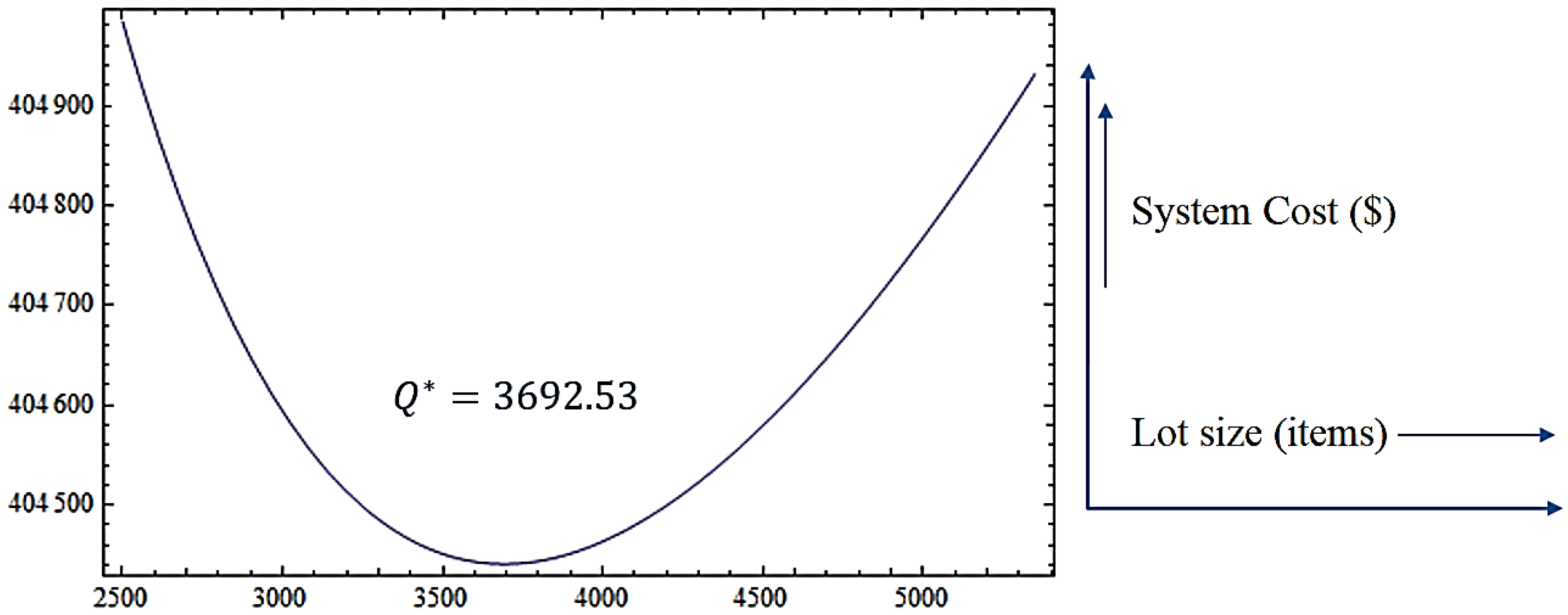
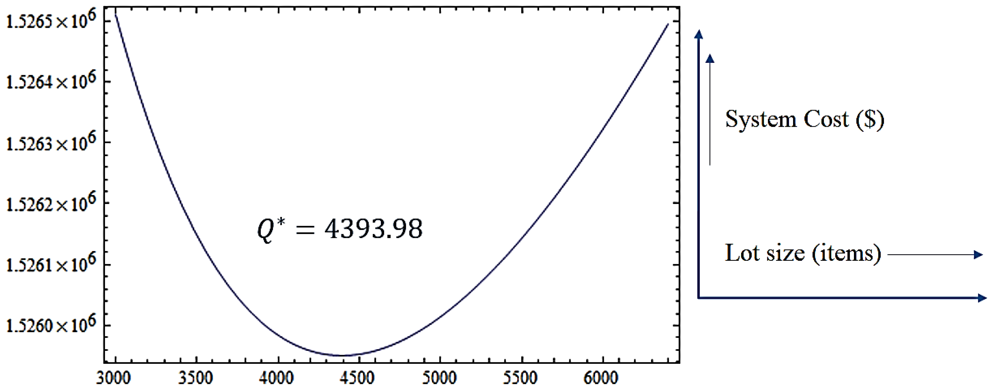
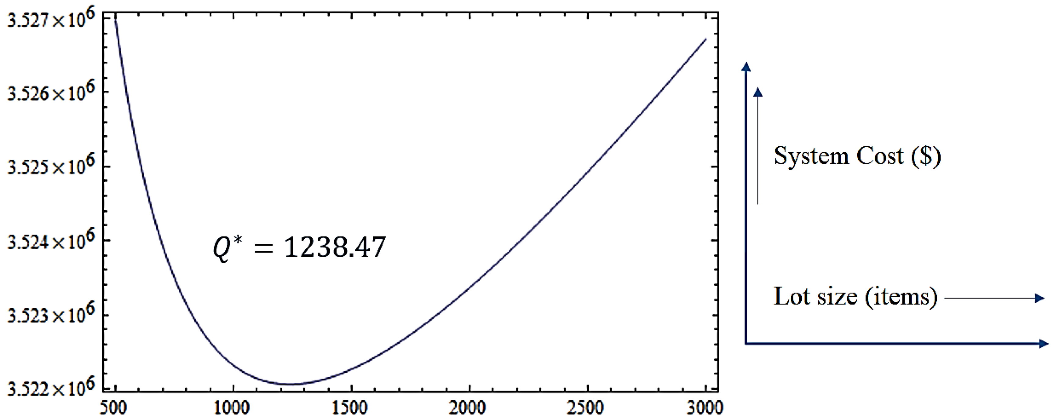
| Five-stage | 3692.53 | 404,441 | 4393.98 | 1,525,950 | 1238.47 | 3,522,058 |
| Parameters | Change (%) | Percentage Change in TC(Q)* | ||||
|---|---|---|---|---|---|---|
| Single-Stage Process | Two-Stage Process | Three-Stage Process | Four-Stage Process | Five-Stage Process | ||
| −50 | −0.73 | −17.09 | −24.92 | −29.53 | −32.57 | |
| −25 | −0.23 | −6.41 | −9.94 | −12.24 | −13.85 | |
| +25 | +0.13 | +4.27 | +7.09 | +9.13 | +10.67 | |
| +50 | +0.21 | +7.33 | +12.40 | +16.20 | +19.15 | |
| −50 | −1.11 | −0.80 | −0.65 | −0.57 | −0.51 | |
| −25 | −0.51 | −0.36 | −0.30 | −0.26 | −0.23 | |
| +25 | +0.45 | +0.32 | +0.26 | +0.23 | +0.21 | |
| +50 | +0.85 | +0.61 | +0.50 | +0.44 | +0.39 | |
| −50 | −47.79 | −48.32 | −48.56 | −48.70 | −48.80 | |
| −25 | −23.89 | −24.16 | −24.28 | −24.35 | −24.40 | |
| +25 | +23.89 | +24.16 | +24.28 | +24.35 | +24.40 | |
| +50 | +47.79 | +48.32 | +48.56 | +48.70 | +48.80 | |
| −50 | −0.32 | −0.32 | −0.32 | −0.32 | −0.33 | |
| −25 | −0.16 | −0.16 | −0.16 | −0.16 | −0.16 | |
| +25 | +0.16 | +0.16 | +0.16 | +0.16 | +0.16 | |
| +50 | +0.32 | +0.32 | +0.32 | +0.32 | +0.33 | |
| −50 | −1.11 | −0.80 | −0.65 | −0.57 | −0.51 | |
| −25 | −0.51 | −0.36 | −0.30 | −0.26 | −0.23 | |
| +25 | +0.45 | +0.32 | +0.26 | +0.23 | +0.21 | |
| +50 | +0.85 | +0.61 | +0.50 | +0.44 | +0.39 | |
| −50 | −0.47 | −0.38 | −0.32 | −0.28 | −0.25 | |
| −25 | −0.24 | −0.19 | −0.16 | −0.14 | −0.12 | |
| +25 | +0.24 | +0.19 | +0.16 | +0.14 | +0.12 | |
| +50 | +0.47 | +0.38 | +0.32 | +0.28 | +0.25 | |
| Parameters | Change (%) | Percentage Change in TC(Q)* | ||||
|---|---|---|---|---|---|---|
| Single-Stage Process | Two-Stage Process | Three-Stage Process | Four-Stage Process | Five-Stage Process | ||
| −50 | −0.17 | −15.12 | −22.75 | −27.42 | −30.57 | |
| −25 | −0.05 | −5.61 | −8.95 | −11.20 | −12.81 | |
| +25 | +0.03 | +3.70 | +6.28 | +8.20 | +9.69 | |
| +50 | +0.05 | +6.33 | +10.94 | +14.48 | +17.28 | |
| −50 | −0.32 | −0.23 | −0.19 | −0.16 | −0.15 | |
| −25 | −0.15 | −0.10 | −0.09 | −0.07 | −0.07 | |
| +25 | +0.13 | +0.09 | +0.08 | +0.07 | +0.06 | |
| +50 | +0.25 | +0.18 | +0.14 | +0.12 | +0.11 | |
| −50 | −48.08 | −48.23 | −48.30 | −48.34 | −48.37 | |
| −25 | −24.04 | −24.12 | −24.15 | −24.17 | −24.18 | |
| +25 | +24.04 | +24.12 | +24.15 | +24.17 | +24.18 | |
| +50 | +48.08 | +48.23 | +48.30 | +48.34 | +48.37 | |
| −50 | −1.37 | −1.38 | −1.38 | −1.38 | −1.38 | |
| −25 | −0.69 | −0.69 | −0.69 | −0.69 | −0.69 | |
| +25 | +0.69 | +0.69 | +0.69 | +0.69 | +0.69 | |
| +50 | +1.37 | +1.38 | +1.38 | +1.38 | +1.38 | |
| −50 | −0.32 | −0.23 | −0.19 | −0.16 | −0.15 | |
| −25 | −0.15 | −0.10 | −0.09 | −0.07 | −0.07 | |
| +25 | +0.13 | +0.09 | +0.08 | +0.07 | +0.06 | |
| +50 | +0.25 | +0.18 | +0.14 | +0.12 | +0.11 | |
| −50 | −0.49 | −0.40 | −0.35 | −0.31 | −0.27 | |
| −25 | −0.24 | −0.20 | −0.17 | −0.15 | −0.14 | |
| +25 | +0.24 | +0.20 | +0.17 | +0.15 | +0.14 | |
| +50 | +0.49 | +0.40 | +0.35 | +0.30 | +0.27 | |
| Parameters | Change (%) | Percentage Change in TC(Q)* | ||||
|---|---|---|---|---|---|---|
| Single-Stage Process | Two-Stage Process | Three-Stage Process | Four-Stage Process | Five-Stage Process | ||
| −50 | −0.10 | −14.38 | −21.92 | −26.61 | −29.80 | |
| −25 | −0.03 | −5.31 | −8.57 | −10.79 | −12.41 | |
| +25 | +0.02 | +3.48 | +5.97 | +7.84 | +9.31 | |
| +50 | +0.03 | +5.95 | +10.37 | +13.80 | +16.55 | |
| −50 | −0.21 | −0.15 | −0.12 | −0.10 | −0.09 | |
| −25 | −0.09 | −0.07 | −0.05 | −0.05 | −0.04 | |
| +25 | +0.08 | +0.06 | +0.05 | +0.04 | +0.04 | |
| +50 | +0.16 | +0.11 | +0.09 | +0.08 | +0.07 | |
| −50 | −49.40 | −49.50 | −49.55 | −49.58 | −49.59 | |
| −25 | −24.70 | −24.75 | −24.77 | −24.79 | −24.80 | |
| +25 | +24.70 | +24.75 | +24.77 | +24.79 | +24.80 | |
| +50 | +49.40 | +49.50 | +49.55 | +49.58 | +49.59 | |
| −50 | −0.25 | −0.25 | −0.25 | −0.25 | −0.25 | |
| −25 | −0.12 | −0.12 | −0.12 | −0.12 | −0.12 | |
| +25 | +0.12 | +0.12 | +0.12 | +0.12 | +0.12 | |
| +50 | +0.25 | +0.25 | +0.25 | +0.25 | +0.25 | |
| −50 | −0.21 | −0.15 | −0.12 | −0.10 | −0.09 | |
| −25 | −0.09 | −0.07 | −0.05 | −0.05 | −0.04 | |
| +25 | +0.08 | +0.06 | +0.05 | +0.04 | +0.04 | |
| +50 | +0.16 | +0.11 | +0.09 | +0.08 | +0.07 | |
| −50 | −0.49 | −0.41 | −0.35 | −0.31 | −0.28 | |
| −25 | −0.25 | −0.20 | −0.18 | −0.16 | −0.14 | |
| +25 | +0.25 | +0.20 | +0.18 | +0.16 | +0.14 | |
| +50 | +0.49 | +0.41 | +0.35 | +0.31 | +0.28 | |
© 2018 by the authors. Licensee MDPI, Basel, Switzerland. This article is an open access article distributed under the terms and conditions of the Creative Commons Attribution (CC BY) license (http://creativecommons.org/licenses/by/4.0/).
Share and Cite
Tayyab, M.; Sarkar, B.; Yahya, B.N. Imperfect Multi-Stage Lean Manufacturing System with Rework under Fuzzy Demand. Mathematics 2019, 7, 13. https://doi.org/10.3390/math7010013
Tayyab M, Sarkar B, Yahya BN. Imperfect Multi-Stage Lean Manufacturing System with Rework under Fuzzy Demand. Mathematics. 2019; 7(1):13. https://doi.org/10.3390/math7010013
Chicago/Turabian StyleTayyab, Muhammad, Biswajit Sarkar, and Bernardo Nugroho Yahya. 2019. "Imperfect Multi-Stage Lean Manufacturing System with Rework under Fuzzy Demand" Mathematics 7, no. 1: 13. https://doi.org/10.3390/math7010013
APA StyleTayyab, M., Sarkar, B., & Yahya, B. N. (2019). Imperfect Multi-Stage Lean Manufacturing System with Rework under Fuzzy Demand. Mathematics, 7(1), 13. https://doi.org/10.3390/math7010013