Introducing Weights Restrictions in Data Envelopment Analysis Models for Mutual Funds

Abstract

Data envelopment analysis has been applied in a number of papers to measure the performance of mutual funds, besides a great many applications on the more diverse fields of performance evaluation. The data envelopment analysis models proposed in the mutual funds literature do not generally set restrictions on the weights assigned to the input and output variables. In this paper, we study the effects of the introduction of different weight restrictions on the results of the performance evaluation of mutual funds. In addition, we provide a unified matrix representation for three widely used approaches on weight restrictions: virtual weight restrictions with constraints on all decision-making units (DMUs) (on all funds); virtual weight restrictions with constraints only on the target unit; assurance regions. Using the unified matrix representation of the weights constraints, we formulate the data envelopment analysis (DEA ) efficiency model and express the efficient frontier in a unified way for the different weight restrictions considered. We investigate the effects of the different weight restrictions on the performance evaluation by means of an empirical application on a set of European mutual funds. Moreover, we study the behaviour of the fund performance scores as the restrictions on the weights become increasingly strict.

1. Introduction

In the last two decades, the data envelopment analysis (DEA) methodology has been applied in different ways to measure the performance of mutual funds, besides a great many applications on the more diverse fields of performance evaluation (more than 10,000 journal articles have been published on DEA; for a recent review, see [1]). By now, there is a wide selection of literature in the mutual funds field, counting more than a hundred papers; for a review, see [2]. In addition, there are many DEA applications to other financial services industry; the majority of studies focus on the banking sector, but several DEA applications to non-banking financial services are also found in the literature; see [3] for a general survey of DEA applications and [4] for recent DEA applications to financial services including mutual funds, banks, insurance, mergers and acquisitions (M&A), and stock selection.

In general, the models proposed in the literature for mutual funds do not impose particular restrictions on the weights of the DEA models, weights which represent the variables of the optimization problems that have to be solved in order to compute the performance scores of the mutual funds analyzed.

Nevertheless, in general DEA models, it is sometimes useful to set proper restrictions on the weights of the input and/or output variables (see, for example, [5,6]).

In this paper, we study the effects of the introduction of different weight restrictions on the results of the performance evaluation of mutual funds.

In addition, a second purpose of this paper is to provide a unified matrix representation for different widely used approaches on weight restrictions, namely:

• virtual weight restrictions with constraints on all decision-making units (DMUs) (see Section 3.1 and Section 4.1);
• virtual weight restrictions with constraints only on the target DMU (see Section 3.1 and Section 4.2);
• weight restrictions with assurance regions (see Section 3.2 and Section 5).

This unified matrix representation enables us to formulate the DEA efficiency model and to express the efficient frontier in a unified way for the models with the different weight restrictions considered (Section 6).

The effects of the different weight restrictions on the performance evaluation of mutual funds are analyzed by carrying out an empirical application on a set of 312 European mutual funds. In the empirical application, we study the behaviour of the fund performance scores as the restrictions on the weights become increasingly strict.

The paper is organized as follows. In Section 2, we define the DEA model without restrictions adopted to evaluate the performance of mutual funds, which will be extended to include weight restrictions in the following sections; this is model DEA-V proposed in [2,7]. The different types of restrictions that can be set on the weights of DEA models are introduced and discussed in Section 3. In Section 4 and Section 5, we derive the matrix representation of the constraints related to the virtual weight restrictions and to assurance regions, respectively. Section 6 defines the DEA efficiency and the efficient frontier for the DEA models with the weight restrictions considered. Section 7 presents the results of the empirical application on European mutual funds carried out and compares the outcomes obtained with the various types of weight restrictions. Finally, Section 8 presents some concluding remarks.

2. An Output Oriented DEA Model for Mutual Funds

Currently, several articles published in the literature have adopted a data envelopment analysis approach to evaluate the performance of mutual funds (see [2] for a review of DEA models for mutual funds and [8] for an introduction to DEA).

Let us start by considering an output oriented DEA model for mutual funds with variable returns to scale that has been proposed in [7] and was extended in [2] to evaluate the performance of a set of European mutual funds.

Let $\{1,2,\dots ,n\}$ indicate the set of mutual funds to be evaluated. Let us denote by $c_{Ij}$ and $c_{Ej}$ the initial and exit fees of an investment in mutual fund $j\in \{1,2,\dots ,n\}$, respectively, and let $K_j$ be the initial payout (net of the initial fee) required by fund j to start with an initial capital equal to 1; moreover, let $M_j$ denote the final value of the investment at the end of the holding period T, net of the exit fee.

The initial payout $K_j$ can be computed as follows:

$$K_j=\frac{1}{1-c_{Ij}}j=1,2,\dots ,n.$$

(1)

If we indicate with $R_j$ the mean instantaneous rate of return of fund j in the investment period $[0,T]$, measured on an annual basis using the continuous compounding law, the final value of the investment $M_j$ can be written as follows:

$$M_j={\mathrm{e}}^{R_{j}T}(1-c_{Ej})j=1,2,\dots ,n.$$

(2)

It is interesting to point out the substantial importance of the initial payout K when the holding period is rather short (say $T\le 1$), while its effect tends to be damped when the duration of the investment increases, as in this latter case the initial fees are spread over several years. Let us also observe that, keeping constant the mean return measured on an annual base, $R_j$, the final value $M_j$ varies exponentially with the length of the holding period T.

The DEA model adopted for the performance evaluation of mutual funds has the final value of the investment M as unique output variable; as for the input variables, the model considers the initial payout K and a set of risk measures that may shed light on different features of the financial risk of mutual funds (see [2]). In this paper, we include two risk measures of the returns of fund j ($j=1,2,\dots ,n$), the $\beta$-coefficient and the downside risk.

The $\beta$-coefficient, ${\beta }_j$, represents the ratio of the covariance between the mutual fund return $R_j$ and the market portfolio return $R_m$ to the variance of the market portfolio return:

$${\beta }_j=\frac{Cov(R_j,R_m)}{Var(R_m)}j=1,2,\dots ,n.$$

(3)

As is well known, the $\beta$-coefficient is relevant as a measure of risk when the investors’ portfolios are well diversified.

On the other hand, the downside risk takes into account the fact that investors see as unfavourable only the lowest returns while the highest ones are welcomed. If we consider as desirable the returns not lower than a target value m, which represents the minimum acceptable return, a proper risk measure is given by the downside risk ${\mathrm{DR}}_{\mathrm{j}}$, defined as the lower semi-deviation of the returns from the target value m:

$${\mathrm{DR}}_{\mathrm{j}}=\sqrt{\frac{1}{T}\sum _{t=1}^T{(\min [r_{jt}-m,0])}^2}j=1,2,\dots ,n.$$

(4)

In the numerical application presented in Section 7, we set m equal to the riskless rate of return.

The input and output variables have been chosen by focusing on the objectives of investors, which are assumed to be risk averse and profit maximizing, as usual in financial theory.

Moreover, the output variable $M_j$ can only take positive values by construction, so that no modification of the model is necessary in order to deal with negative output data. Even if some of the values of the input variable beta may sometimes be negative, the problem of negative input data can easily be overcome by translating the beta variable adding a suitable positive constant; indeed, it is well known that the variable returns to scale DEA model with output orientation is translation invariant with respect to inputs (see [8], p. 94).

The use of a DEA model leads to the determination of an efficiency score for each mutual fund, which is computed as the highest value of the ratio of the weighted sum of outputs to the weighted sum of inputs (see e.g., [8]).

There are various typologies of DEA models, which differ with respect to the type of returns to scale and the orientation. In this paper, we consider a DEA model with variable returns to scale and an output orientation; for the appropriateness of the choice of an output oriented DEA model with variable returns to scale for the evaluation of mutual funds, see [2,7].

In such a case, the efficiency score for each mutual fund $o\in \{1,2,\dots ,n\}$ is the optimal value $\mathrm{DEA}-{\mathrm{V}}_o^{*}$ of the objective function of the following fractional programming problem:

$$\underset{\{u,v_i\}}{\max }\frac{u{M}_o}{v_1{K}_o+v_2{\beta }_o+v_3{\mathrm{DR}}_{\mathrm{o}}-v_0},$$

(5)

subject to

$$\begin{array}{cc}\hfill & \frac{u{M}_j}{v_1{K}_j+v_2{\beta }_j+v_3{\mathrm{DR}}_{\mathrm{j}}-v_0}\le 1,j=1,2,\dots ,n,\hfill \end{array}$$

(6)

$$\begin{array}{cc}\hfill & u\ge \epsilon ,\hfill \end{array}$$

(7)

$$\begin{array}{cc}\hfill & v_i\ge \epsilon i=1,2,3,\hfill \end{array}$$

(8)

where u is the weight assigned to the final value $M_j$, $v_1$ is the weight assigned to the initial payout $K_j$, $v_2$ and $v_3$ are the weights assigned to the $\beta$-coefficient ${\beta }_j$ and the downside risk ${\mathrm{DR}}_{\mathrm{j}}$, respectively, and $v_0$ characterizes the variable returns to scale models.

$\epsilon$ is a non-Archimedean infinitesimal that prevents the weights from vanishing and is introduced in order to prevent that, under particular conditions, units that are not efficient are incorrectly declared as efficient (see [9]). Actually, the DEA efficiency requires not only that the efficiency score $\mathrm{DEA}-{\mathrm{V}}_o^{*}$ reaches its maximum value, equal to 1 because of constraint (6), but also that it is not possible to achieve this result by reducing an input or augmenting an output while maintaining the value of the other inputs and outputs constant (see, for example, [8]).

As is usual in fractional programming, to solve models (5)–(8), we can conveniently transform it into an equivalent linear programming problem. By adopting the output orientation, we can write the following equivalent linear programming problem:

$$\underset{\{u,v_i\}}{\min }{v}_1{K}_o+v_2{\beta }_o+v_3{\mathrm{DR}}_{\mathrm{o}}-v_0,$$

(9)

subject to

$$\begin{array}{cc}\hfill & u{M}_o=1,\hfill \end{array}$$

(10)

$$\begin{array}{cc}\hfill & v_1{K}_j+v_2{\beta }_j+v_3{\mathrm{DR}}_{\mathrm{j}}-u{M}_j-v_0\ge 0j=1,2,\dots ,n,\hfill \end{array}$$

(11)

$$\begin{array}{cc}\hfill & u\ge \epsilon ,\hfill \end{array}$$

(12)

$$\begin{array}{cc}\hfill & v_i\ge \epsilon i=1,2,3,\hfill \end{array}$$

(13)

where the numerator of the objective function ratio (5) is set equal to 1 (constraint (10)) and we minimize the denominator. The efficiency score of mutual fund o coincides with the reciprocal of the optimal function value (5).

The dual of problems (9)–(13) can be written as follows:

$$\max z_0+\epsilon (s^{+}+\sum _{i=1}^3{s}_i^{-}),$$

(14)

subject to

$$\begin{array}{cc}\hfill & M_o{z}_0-\sum _{j=1}^n{M}_j{\lambda }_j+s^{+}=0,\hfill \end{array}$$

(15)

$$\begin{array}{cc}\hfill & \sum _{j=1}^n{K}_j{\lambda }_j+s_1^{-}=K_o,\hfill \end{array}$$

(16)

$$\begin{array}{cc}\hfill & \sum _{j=1}^n{\beta }_j{\lambda }_j+s_2^{-}={\beta }_o,\hfill \end{array}$$

(17)

$$\begin{array}{cc}\hfill & \sum _{j=1}^n{\mathrm{DR}}_{\mathrm{j}}{\lambda }_j+s_3^{-}={\mathrm{DR}}_{\mathrm{o}},\hfill \end{array}$$

(18)

$$\begin{array}{cc}\hfill & \sum _{j=1}^n{\lambda }_j=1,\hfill \end{array}$$

(19)

$$\begin{array}{cc}\hfill & {\lambda }_j\ge 0j=1,2,\dots ,n,\hfill \end{array}$$

(20)

$$\begin{array}{cc}\hfill & s^{+}\ge 0,s_i^{-}\ge 0i=1,2,3,\hfill \end{array}$$

(21)

where $z_0$ is the dual variable associated with the equality constraint (10), ${\lambda }_j$ are the dual variables associated with constraints (11), $s^{+}$ is the dual variable associated with the output weight constraint (12) and $s_i^{-}$ (for $i=1,2,3$) are the dual variables associated with the input weight constraints (13). The dual variables $s^{+}$ and $s_i^{-}$ associated with the output and input weight constraints are usually called slacks since they can just be interpreted as slacks of the dual constraints in which they appear.

Let us observe that in problems (14)–(21) the convexity constraint (19), ${\sum }_{j=1}^n{\lambda }_j=1$, means that we restrict the set of benchmark portfolios that can be considered to the convex hull of the funds analyzed, so that only convex combinations of the existing funds are allowed.

The dual problems (14)–(21) is the one commonly used to compute the efficiency score and determine the efficient units. The efficiency score of mutual fund o is given by the reciprocal of the optimal value of $z_0$, i.e., $\mathrm{DEA}-{\mathrm{V}}_o^{*}=1/z_0^{*}$.

It is known that the presence in programs (14)–(21) of the non-Archimedean infinitesimal $\epsilon$ may cause computational problems when, as it is often done in commercial softwares, it is replaced by a small positive real number (for instance ${10}^{-6}$); see [10,11]. In order to overcome these problems, it is possible to use a special two-phase procedure that avoids using the non-Archimedean infinitesimal $\epsilon$ by splitting the process of efficiency evaluation in two subsequent linear programs (see [12]); the two-phase procedure has the advantage of reducing the computational drawbacks while providing the same efficiency characterization (see [8] (pp. 46, 73–75)).

The two-phase procedure tackles the linear program in dual form; in Phase I, we solve the following linear program:

Phase I

$$\max z_0,$$

(22)

subject to

$$\begin{array}{cc}\hfill & M_o{z}_0-\sum _{j=1}^n{M}_j{\lambda }_j+s^{+}=0,\hfill \end{array}$$

(23)

$$\begin{array}{cc}\hfill & \sum _{j=1}^n{K}_j{\lambda }_j+s_1^{-}=K_o,\hfill \end{array}$$

(24)

$$\begin{array}{cc}\hfill & \sum _{j=1}^n{\beta }_j{\lambda }_j+s_2^{-}={\beta }_o,\hfill \end{array}$$

(25)

$$\begin{array}{cc}\hfill & \sum _{j=1}^n{\mathrm{DR}}_{\mathrm{j}}{\lambda }_j+s_3^{-}={\mathrm{DR}}_{\mathrm{o}},\hfill \end{array}$$

(26)

$$\begin{array}{cc}\hfill & \sum _{j=1}^n{\lambda }_j=1,\hfill \end{array}$$

(27)

$$\begin{array}{cc}\hfill & {\lambda }_j\ge 0,j=1,2,\dots ,n,\hfill \end{array}$$

(28)

$$\begin{array}{cc}\hfill & s^{+}\ge 0,s_i^{-}\ge 0i=1,2,3,\hfill \end{array}$$

(29)

which differs from the dual problems (14)–(21) only because its objective function lacks the term $\epsilon (s^{+}+{\sum }_{i=1}^3{s}_i^{-})$. With respect to the primal program, this corresponds to replace the constraints (12) and (13) involving $\epsilon$ with simple non-negativity constraints on the input and output weights.

Let $z_0^{*}$ be the optimal solution of the Phase I problem (22)–(29). In order to see whether a fund with $z_0^{*}=1$ is fully efficient, we need to check if it is not possible to achieve the same score by increasing an output and maintaining the value of the other inputs and outputs constant. In terms of linear programs, this entails checking that there exists a solution for problems (14)–(21) with all the output and input slacks, $s^{+}$ and $s_i^{-}$, equal to zero, and this can be done by solving the following Phase II problem in which $z_0$ is set equal to its optimal value achieved in Phase I, $z_0^{*}$:

Phase II

$$\max s^{+}+\sum _{i=1}^3{s}_i^{-},$$

(30)

subject to

$$\begin{array}{cc}\hfill & M_o{z}_0^{*}-\sum _{j=1}^n{M}_j{\lambda }_j+s^{+}=0,\hfill \end{array}$$

(31)

$$\begin{array}{cc}\hfill & \sum _{j=1}^n{K}_j{\lambda }_j+s_1^{-}=K_o,\hfill \end{array}$$

(32)

$$\begin{array}{cc}\hfill & \sum _{j=1}^n{\beta }_j{\lambda }_j+s_2^{-}={\beta }_o,\hfill \end{array}$$

(33)

$$\begin{array}{cc}\hfill & \sum _{j=1}^n{\mathrm{DR}}_{\mathrm{j}}{\lambda }_j+s_3^{-}={\mathrm{DR}}_{\mathrm{o}},\hfill \end{array}$$

(34)

$$\begin{array}{cc}\hfill & \sum _{j=1}^n{\lambda }_j=1,\hfill \end{array}$$

(35)

$$\begin{array}{cc}\hfill & {\lambda }_j\ge 0,j=1,2,\dots ,n,\hfill \end{array}$$

(36)

$$\begin{array}{cc}\hfill & s^{+}\ge 0,s_i^{-}\ge 0i=1,2,3.\hfill \end{array}$$

(37)

In conclusion, a mutual fund o is efficient if and only if $z_0^{*}=1$ and the optimal value of the Phase II objective function (30) is equal to 0.

3. Restrictions on the Weights of a DEA Model

One of the main features of standard DEA models lies in the weight flexibility, which means that the models look for the optimal values of input and output weights and maximize the efficiency of the target unit without imposing particular restrictions on the weights; only positivity constraints such as constraints (12) and (13) are usually considered.

This fundamental feature of the DEA approach allows for highlighting the input and output variables that put in the best light the units examined, but it may sometimes lead to some drawbacks in the performance evaluation process. For example, a given unit may be evaluated as efficient despite having very high values of some inputs. In the DEA applications to mutual funds, for example, this could cause an investment fund to be assessed as efficient despite exhibiting a very high risk or requiring a very high initial payout (because of a high initial fee). In a different situation, if we need to evaluate the performance of socially responsible investment funds and we include a measure of the fund social responsibility as an additional output ([7]), a fund could be stated as efficient although its involvement in social responsibility is negligible, or it could be declared efficient even though its final value is very low.

In the cases in which it is advisable to ensure that we do not neglect some important input and output variables in the efficiency analysis, we can introduce some appropriate restrictions on the weights associated with these variables in the DEA model.

Moreover, a second reason that may suggest the introduction of additional weight restrictions in the DEA model is to somehow take into account eventual preference information of decision makers or experts on the respective importance of the variables that can be synthesized in a range for the weights.

It may be shown that the weight restrictions suggested in the literature often lead to models with a greater discriminatory power (see, for example, [13]) that provide a lower number of efficient decision-making units (DMUs). Especially when the number of DMUs is low, this feature may represent a third motivation for adopting a DEA model with weight restrictions; an example of an effective increase in the discrimination obtained with weight restrictions is presented in [14].

Several typologies of weight restrictions have been proposed in the DEA literature to reduce weight flexibility (for a review, see Allen et al. [5] and Thanassoulis et al. [6]).

A simple approach is given by the so-called absolute weight restrictions, which consists of lower and upper bounds set directly on the value of the input and output weights ([15]):

$$\begin{array}{cc}\hfill & L_i^X\le v_i\le U_i^X(i=1,\dots ,m),\hfill \end{array}$$

(38)

$$\begin{array}{cc}\hfill & L_r^Y\le u_r\le U_r^Y(r=1,\dots ,t),\hfill \end{array}$$

(39)

where $L_i^X$ and $U_i^X$ are the lower and upper bounds imposed on the input weight $v_i$ and $L_r^Y$ and $U_r^Y$ are the analogous bounds of the output weight $u_r$.

These constraints are simple, but, on the other hand, the meaning of the bounds may be not always clear; moreover, they can give rise to infeasibility problems.

Two other well known types of weight restrictions will be described more in detail in the following part of this section since the remaining of this paper will be focused on them.

3.1. Virtual Weight Restrictions

Another approach imposes lower and upper limits not directly on the value of the weights but rather on the proportional contribution of the virtual inputs or outputs to the overall weighted sum of inputs or outputs. These kinds of restrictions are called virtual weights (VW, in brief) restrictions and were proposed by Wong and Beasley [16]; see also Sarrico and Dyson [17] for further details.

In general, let us consider a DEA model with n DMUs employing m inputs to produce t outputs. Let us denote by $y_{rj}$ the amount of output r ($r=1,\cdots ,t$) produced by DMU j ($j=1,\cdots ,n$) and by $x_{ij}$ the amount of input i ($i=1,\cdots ,m$) used by the same DMU. The virtual input related to the i-th input variable for DMU j is defined as the product of the level of the input and the corresponding optimal weight $v_i$), i.e., $v_i{x}_{ij}$. Analogously, the virtual output related to the r-th output variable is defined as the product of the level of the output and the corresponding optimal weight $u_r$), $u_r{y}_{rj}$.

The virtual weight restrictions applied to inputs restrict the proportion of each virtual input with respect to the total virtual input:

$${\displaystyle L_{i^{\prime }}^X\le \frac{v_{i^{\prime }}{x}_{i^{\prime }j}}{{\sum }_{i=1}^m{v}_i{x}_{ij}}\le U_{i^{\prime }}^X(i^{\prime }=1,\dots ,m;j=1,\dots ,n),}$$

(40)

where $L_{i^{\prime }}^X$ and $U_{i^{\prime }}^X$ are the lower and upper percentage values that limit the virtual input $i^{\prime }$; for example, we may require that the proportion of the total virtual input for the first input variable falls between $20\%$ and $80\%$.

Analogous proportional restrictions may be defined for the virtual outputs, too:

$${\displaystyle L_{r^{\prime }}^Y\le \frac{u_{r^{\prime }}{y}_{r^{\prime }j}}{{\sum }_{r=1}^t{u}_r{y}_{rj}}\le U_{r^{\prime }}^Y(r^{\prime }=1,\dots ,t;j=1,\dots ,n),}$$

(41)

where $L_{r^{\prime }}^Y$ and $U_{r^{\prime }}^Y$ are the lower and upper percentage values set for the virtual output $r^{\prime }$.

Let us remark that the virtual weight restrictions can be easily interpreted and therefore it is more straightforward to assign reasonable numerical values to the lower and upper bounds. In the case of a DEA model for mutual fund assessment, for instance, by setting lower bounds on the proportion of the virtual input, we may require that each risk measure contribute to the total virtual input for at least a minimum percentage and for not more than a maximum percentage and that similar percentage restrictions hold for the initial payout.

Notice that, in the case of models (5)–(8), it has little meaning to assign proportional weights restriction to the (single) virtual output. Nevertheless, in the following, we will present both input and output restrictions, which are also useful for more general models. For mutual funds, in particular, a general treatment can be used to generalize the DEA model including multiple output variables; with regard to that, we may refer to the DEA models for socially responsible investment funds ([7]).

It is straightforward to write the lower and upper constraints (40) and (41) in an equivalent linear form, more convenient to add to the linear constraints of a DEA primal problem:

$$\begin{array}{cc}{\displaystyle -\sum _{i=1}^m{v}_i(L_{i^{\prime }}^X{x}_{ij})+v_{i^{\prime }}{x}_{i^{\prime }j}\ge 0}& (i^{\prime }=1,\dots ,m;j=1,\dots ,n),\hfill \end{array}$$

(42)

$$\begin{array}{cc}{\displaystyle \sum _{i=1}^m{v}_i(U_{i^{\prime }}^X{x}_{ij})-v_{i^{\prime }}{x}_{i^{\prime }j}\ge 0}& (i^{\prime }=1,\dots ,m;j=1,\dots ,n),\hfill \end{array}$$

(43)

and, respectively,

$$\begin{array}{cc}{\displaystyle -\sum _{r=1}^t{u}_r(L_{r^{\prime }}^Y{y}_{rj})+u_{r^{\prime }}{y}_{r^{\prime }j}\ge 0}& (r^{\prime }=1,\dots ,t;j=1,\dots ,n),\hfill \end{array}$$

(44)

$$\begin{array}{cc}{\displaystyle \sum _{r=1}^t{u}_r(U_{r^{\prime }}^Y{y}_{rj})-u_{r^{\prime }}{y}_{r^{\prime }j}\ge 0}& (r^{\prime }=1,\dots ,t;j=1,\dots ,n).\hfill \end{array}$$

(45)

3.2. Restrictions with Assurance Regions

In the DEA practice, the most commonly used restrictions are given by the so called assurance regions (AR) ([18]), which impose restrictions on the ratios between the weights of inputs and/or outputs. More specifically, Type I assurance regions consider lower and upper bounds on the ratio between the weights of either the inputs:

$${\displaystyle L_{i^{\prime }i}^X\le \frac{v_i}{v_{i^{\prime }}}\le U_{i^{\prime }i}^X(i^{\prime }=1,\dots ,m;i=1,\dots ,m)}$$

(46)

or the outputs:

$${\displaystyle L_{r^{\prime }r}^Y\le \frac{u_r}{u_{r^{\prime }}}\le U_{r^{\prime }r}^Y(r^{\prime }=1,\dots ,t;r=1,\dots ,t),}$$

(47)

where $L_{i^{\prime }i}^X$ and $U_{i^{\prime }i}^X$ are non-negative lower and upper bounds that limit the ratio of the input weights $\frac{v_i}{v_{i^{\prime }}}$ and, analogously, $L_{r^{\prime }r}^Y$ and $U_{r^{\prime }r}^Y$ are the bounds of the output weights ratio $\frac{u_r}{u_{r^{\prime }}}$. Notice that for $i^{\prime }=i$ and $r^{\prime }=r$ the lower bounds may take any non-negative value lower than or equal to 1 and the upper bounds may take any value greater than or equal to 1 and the restrictions are redundant. Of course, a lower bound equal to 0 corresponds to the case without a limitation from below.

In addition, once the lower bounds are set, the upper bounds are redundant since they can be derived from the lower bounds; indeed, if we take the reciprocal of a weights ratio, we have:

$$L_{i^{\prime }i}^X\le \frac{v_i}{v_{i^{\prime }}}\iff \frac{v_{i^{\prime }}}{v_i}\le \frac{1}{L_{i^{\prime }i}^X}$$

(48)

so that $U_{i{i}^{\prime }}^X=\frac{1}{L_{i^{\prime }i}^X}$. In general, we have:

$$\begin{array}{cc}\hfill & {\displaystyle U_{i{i}^{\prime }}^X=\frac{1}{L_{i^{\prime }i}^X}(i^{\prime }=1,\dots ,m;i=1,\dots ,m),}\hfill \end{array}$$

(49)

$$\begin{array}{cc}\hfill & {\displaystyle U_{r{r}^{\prime }}^Y=\frac{1}{L_{r^{\prime }r}^Y}(r^{\prime }=1,\dots ,t;r=1,\dots ,t)}\hfill \end{array}$$

(50)

and constraints (46) and (47) can be equivalently written in linear forms as follows:

$${\displaystyle v_i-L_{i^{\prime }i}^X{v}_{i^{\prime }}\ge 0(i^{\prime }=1,\dots ,m;i=1,\dots ,m)}$$

(51)

and

$${\displaystyle u_r-L_{r^{\prime }r}^Y{u}_{r^{\prime }}\ge 0(r^{\prime }=1,\dots ,t;r=1,\dots ,t).}$$

(52)

We remark that in the literature very often type I assurance regions are defined using a more parsimonious representation which takes into consideration only the weights ratios computed with respect to one of the weights, usually the first one ( for example [8]):

$$\begin{array}{cc}\hfill & {\displaystyle L_{1i}^X\le \frac{v_i}{v_1}\le U_{1i}^X(i=2,\dots ,m),}\hfill \end{array}$$

(53)

$$\begin{array}{cc}\hfill & {\displaystyle L_{1r}^Y\le \frac{u_r}{u_1}\le U_{1r}^Y(r=2,\dots ,t).}\hfill \end{array}$$

(54)

The restrictions considered in Type I assurance regions may be appropriate when these restrictions come from a production technology that provides some technological information on the marginal rates of technical substitution between the inputs or the outputs.

We may cite another type of restrictions that falls in the assurance regions category, even if we will not use them for mutual funds; they impose cross restrictions that link input and output weights and give rise to the so called Type II assurance regions; for example, [5].

4. Matrix Representation of Virtual Weights Restrictions

In Section 3, we have presented two different ways to define restrictions on the weights of a DEA model incorporating some value judgements conveyed by experts or decision makers. In the present and the next sections, we derive a matrix representation for these restrictions that will be incorporated in the DEA models in Section 6.

In particular, in this section, we focus on the virtual weight restrictions (42)–(45), which seem better fit for the performance evaluation of mutual funds.

First of all, let us observe that in general there are two different ways to impose VW restrictions in a DEA model, since we may either impose only the input and output constraints regarding the target DMU o or we may impose the constraints regarding all the DMUs under analysis simultaneously. In the first case, the number of constraints that are added is equal to $2(m+t)$. In the second case, this number is multiplied by the number n of DMUs, i.e., it is $2(m+t)n$. The first case is computationally less cumbersome, but it has the serious drawback that the projection on the efficient frontier of a non efficient DMU may not satisfy the virtual weights constraints (see, e.g., [14]).

On the other hand, the case in which the VW constraints are imposed for all DMUs simultaneously ensures that this projection satisfies all the constraints (indeed, all the necessary constraints are present in the optimization problem), but at the cost of a more cumbersome optimization problem. Moreover, the high number of constraints included may sometimes lead to infeasibility problems, if the lower and upper bounds in the VW constraints are too strict.

Let us now write in a convenient matrix form the VW constraints (42)–(45). Let $X=(x_{ij})$ be the $m\times n$ matrix of inputs, $Y=(x_{rj})$ be the $t\times n$ matrix of outputs, $v=(v_1,\dots ,v_m)$ be the row vector of the input weights, $u=(u_1,\dots ,u_t)$ be the row vector of the output weights, $L^X=(L_1^X,\dots ,L_m^X)$ be the row vector of the lower bounds on the proportional virtual inputs, $U^X=(U_1^X,\dots ,U_m^X)$ be the row vector of the upper bounds on the proportional virtual inputs, $L^Y=(L_1^Y,\dots ,L_t^Y)$ be the row vector of the lower bounds on the proportional virtual outputs, $U^Y=(U_1^Y,\dots ,U_t^Y)$ be the row vector of the upper bounds on the proportional virtual outputs.

Let us start with the input constraints. Constraint (42) can be equivalently written in matrix form in the following way:

$$v{P}_j^L\ge \mathbf{0}(j=1,\dots ,n),$$

(55)

where $\mathbf{0}\in {\mathbb{R}}^m$ is a null row vector and $P_j^L$ is the following $m\times m$ matrix:

$$P_j^L=\left(\begin{array}{cccc}(-L_1^X+1)x_{1j}& -L_2^X{x}_{1j}& \dots & -L_m^X{x}_{1j}\\ -L_1^X{x}_{2j}& (-L_2^X+1)x_{2j}& \dots & -L_m^X{x}_{2j}\\ & ⋮& & \\ -L_1^X{x}_{mj}& -L_2^X{x}_{mj}& \dots & (-L_m^X+1)x_{mj}\end{array}\right)=D_j^X-x_j{L}^X.$$

(56)

$x_j={(x_{1j},\dots ,x_{mj})}^{\prime }$ is the j-th column of the input matrix X and $D_j^X$ is the diagonal matrix with the elements of $x_j$ on the main diagonal.

Constraint (43) can be written in matrix form as follows:

$$v{P}_j^U\ge \mathbf{0}(j=1,\dots ,n),$$

(57)

where $P_j^U$ is the following $m\times m$ matrix:

$$P_j^U=\left(\begin{array}{cccc}(U_1^X-1)x_{1j}& U_2^X{x}_{1j}& \dots & U_m^X{x}_{1j}\\ U_1^X{x}_{2j}& (U_2^X-1)x_{2j}& \dots & U_m^X{x}_{2j}\\ & ⋮& & \\ U_1^X{x}_{mj}& U_2^X{x}_{mj}& \dots & (U_m^X-1)x_{mj}\end{array}\right)=-D_j^X+x_j{U}^X.$$

(58)

In a similar manner, we may write in matrix form the output constraints. Constraint (44) is equivalent to:

$$u{Q}_j^L\ge \mathbf{0}(j=1,\dots ,n);$$

(59)

here, $\mathbf{0}\in {\mathbb{R}}^t$, $Q_j^L$ is the $t\times t$ matrix:

$$Q_j^L=\left(\begin{array}{cccc}(-L_1^Y+1)y_{1j}& -L_2^Y{y}_{1j}& \dots & -L_t^Y{y}_{1j}\\ -L_1^Y{y}_{2j}& (-L_2^Y+1)y_{2j}& \dots & -L_t^Y{y}_{2j}\\ & ⋮& & \\ -L_1^Y{y}_{tj}& -L_2^Y{y}_{tj}& \dots & (-L_t^Y+1)y_{tj}\end{array}\right)=D_j^Y-y_j{L}^Y.$$

(60)

$y_j={(y_{1j},\dots ,y_{tj})}^{\prime }$ is the j-th column of the output matrix Y and $D_j^Y$ is the diagonal matrix with the elements of $y_j$ on the main diagonal.

Constraint (45) can be written as follows:

$$u{Q}_j^U\ge \mathbf{0}(j=1,\dots ,n),$$

(61)

where $Q_j^U$ is the following $t\times t$ matrix:

$$Q_j^U=\left(\begin{array}{cccc}(U_1^Y-1)y_{1j}& U_2^Y{y}_{1j}& \dots & U_t^Y{y}_{1j}\\ U_1^Y{y}_{2j}& (U_2^Y-1)y_{2j}& \dots & U_t^Y{y}_{2j}\\ & ⋮& & \\ U_1^Y{y}_{tj}& U_2^Y{y}_{tj}& \dots & (U_t^Y-1)y_{tj}\end{array}\right)=-D_j^Y+y_j{U}^Y.$$

(62)

We have seen that in the DEA optimization problem for the computation of the efficiency score of the target DMU o (let us recall that the DEA approach requires the solution of an optimization problem for each of the DMUs analyzed) we may either simultaneously impose the VW input and output constraints regarding all DMUs or we may consider only the constraints regarding the target DMU. Of course, the choice of the first or the second alternative leads to different representations of the constraints to be included in the DEA optimization problem. Let us thus examine the two alternatives separately.

4.1. Case 1: Constraints on All DMUs

In the first case, the constraints to be added to the optimization problem that allows us to compute the efficiency score of DMU o (with $o\in \{1,2,\dots ,n\}$) are the same for all DMUs, since the VW constraints of all DMUs are present in the optimization problems to compute the efficiency scores of all DMUs:

$$\begin{array}{cc}\hfill & v{P}_j^L\ge \mathbf{0}(j=1,\dots ,n),\hfill \end{array}$$

(63)

$$\begin{array}{cc}\hfill & v{P}_j^U\ge \mathbf{0}(j=1,\dots ,n),\hfill \end{array}$$

(64)

$$\begin{array}{cc}\hfill & u{Q}_j^L\ge \mathbf{0}(j=1,\dots ,n),\hfill \end{array}$$

(65)

$$\begin{array}{cc}\hfill & u{Q}_j^U\ge \mathbf{0}(j=1,\dots ,n).\hfill \end{array}$$

(66)

It is immediate to see that constraint (63) can be written in matrix form as follows:

$$v{P}^L\ge \mathbf{0},$$

(67)

where $\mathbf{0}\in {\mathbb{R}}^{m\times n}$ and $P^L$ is the following $m\times (mn)$ matrix:

$$P^L=\left(P_1^L{P}_2^L\dots P_n^L\right).$$

(68)

Analogously, constraint (64) can be written as:

$$v{P}^U\ge \mathbf{0},$$

(69)

where $P^U$ is the $m\times (mn)$ matrix:

$$P^U=\left(P_1^U{P}_2^U\dots P_n^U\right);$$

(70)

constraint (65) can be written as:

$$u{Q}^L\ge \mathbf{0},$$

(71)

where $\mathbf{0}\in {\mathbb{R}}^{t\times n}$ and $Q^L$ is the following $t\times (tn)$ matrix:

$$Q^L=\left(Q_1^L{Q}_2^L\dots Q_n^L\right)$$

(72)

and constraint (66) can be written as:

$$u{Q}^U\ge \mathbf{0},$$

(73)

where $Q^U$ is the $t\times (tn)$ matrix:

$$Q^U=\left(Q_1^U{Q}_2^U\dots Q_n^U\right).$$

(74)

4.2. Case 2: Constraints Only on the Target DMU

In the second case, the constraints to be added to the optimization problem that allows us to compute the efficiency score of DMU o (with $o\in \{1,2,\dots ,n\}$) are only those related to the target DMU o:

$$\begin{array}{cc}\hfill & v{P}_o^L\ge \mathbf{0},\hfill \end{array}$$

(75)

$$\begin{array}{cc}\hfill & v{P}_o^U\ge \mathbf{0},\hfill \end{array}$$

(76)

$$\begin{array}{cc}\hfill & u{Q}_o^L\ge \mathbf{0},\hfill \end{array}$$

(77)

$$\begin{array}{cc}\hfill & u{Q}_o^U\ge \mathbf{0}.\hfill \end{array}$$

(78)

To use the same matrix notation adopted in case 1, by setting $P^L=P_o^L$, $P^U=P_o^U$, $Q^L=Q_o^L$, $Q^U=Q_o^U$, we can write equivalently:

$$\begin{array}{cc}\hfill & v{P}^L\ge \mathbf{0},\hfill \end{array}$$

(79)

$$\begin{array}{cc}\hfill & v{P}^U\ge \mathbf{0},\hfill \end{array}$$

(80)

$$\begin{array}{cc}\hfill & u{Q}^L\ge \mathbf{0},\hfill \end{array}$$

(81)

$$\begin{array}{cc}\hfill & u{Q}^U\ge \mathbf{0},\hfill \end{array}$$

(82)

where it is clear that the constraints on the proportional virtual weights can be written in a similar form for cases 1 and 2, only the construction of the matrices $P^L,P^U,Q^L,Q^U$ involved changes.

5. Matrix Representation of Assurance Region Weight Restrictions

It is possible to represent in a matrix form analogous to (79)–(82) also the weight restrictions (51) and (52) defined with the assurance region method. This will allow us to proceed with a unified formulation of the DEA programs in the next section.

Of course, for our representation of the assurance regions, we may set $P^U$ and $Q^U$ equal to null matrices. As for the matrices $P^L$ and $Q^L$, to see how they can be written, let us first write the matrix $P^L$ in the case $m=3$:

$$P^L=\left(\begin{array}{ccccccccc}0& 1& 1& -L_{21}^X& 0& 0& -L_{31}^X& 0& 0\\ 0& -L_{12}^X& 0& 1& 0& 1& 0& -L_{32}^X& 0\\ 0& 0& -L_{13}^X& 0& 0& -L_{23}^X& 1& 1& 0\end{array}\right).$$

(83)

By examining this matrix, we can see that, in the general case, $P^L$ can be written as the $m\times m^2$ matrix:

$$P^L=\left(P_1^L{P}_2^L\dots P_m^L\right),$$

(84)

where the submatrices $P_i^L$ are $m\times m$ matrices defined as follows:

$$P_i^L=I_i^X-{\overline{D}}_i^X,$$

(85)

with $I_i^X$ defined as the $m\times m$ matrix with the elements in the i-th row equal to 1 and all the other elements equal to 0 and ${\overline{D}}_i^X$ is the $m\times m$ diagonal matrix with the lower bounds $L_{i1}^X,L_{i2}^X,\dots ,L_{im}^X$ on the main diagonal; here, we set $L_{ii}^X=1$.

Analogously, $Q^L$ can be written as the $t\times t^2$ matrix:

$$Q^L=\left(Q_1^L{Q}_2^L\dots Q_t^L\right),$$

(86)

where the submatrices $Q_r^L$ are $t\times t$ matrices defined as:

$$Q_r^L=I_r^Y-{\overline{D}}_r^Y,$$

(87)

with $I_r^Y$ defined as the $t\times t$ matrix with the elements in the r-th row equal to 1 and all the other elements equal to 0 and ${\overline{D}}_r^Y$ is the $t\times t$ diagonal matrix with the lower bounds $L_{r1}^Y,L_{r2}^Y,\dots ,L_{rt}^Y$ on the main diagonal; here, $L_{rr}^Y=1$.

6. DEA Efficiency Evaluation with Virtual Weights Restrictions and Assurance Regions

We are finally ready to incorporate the weight restrictions that have been discussed in the previous sections in a general DEA output oriented model with either constant or variable returns to scale in matrix form.

We have been able to represent both the virtual weight restrictions (for either case 1 or case 2) and the assurance regions in the following compact form:

$$\begin{array}{cc}\hfill & v{P}^L\ge \mathbf{0},\hfill \end{array}$$

(88)

$$\begin{array}{cc}\hfill & v{P}^U\ge \mathbf{0},\hfill \end{array}$$

(89)

$$\begin{array}{cc}\hfill & u{Q}^L\ge \mathbf{0},\hfill \end{array}$$

(90)

$$\begin{array}{cc}\hfill & u{Q}^U\ge \mathbf{0}.\hfill \end{array}$$

(91)

Let us consider the general output oriented DEA model in the two-phase dual formulation. We can take into account these constraints in the Phase I problem, which can be written in the following way:

$$\max z_o,$$

(92)

subject to

$$\begin{array}{cc}\hfill & X\lambda +P^L{\rho }^L+P^U{\rho }^U+s^{-}=x_o,\hfill \end{array}$$

(93)

$$\begin{array}{cc}\hfill & z_o{y}_o-Y\lambda +Q^L{\tau }^L+Q^U{\tau }^U+s^{+}=\mathbf{0},\hfill \end{array}$$

(94)

$$\begin{array}{cc}\hfill & \mathbf{1}\lambda =1,\hfill \end{array}$$

(95)

$$\begin{array}{cc}\hfill & \lambda \ge \mathbf{0},{\rho }^L\ge \mathbf{0},{\rho }^U\ge \mathbf{0},{\tau }^L\ge \mathbf{0},{\tau }^U\ge \mathbf{0},s^{-}\ge \mathbf{0},s^{+}\ge \mathbf{0},\hfill \end{array}$$

(96)

where ${\rho }^L$, ${\rho }^U$, ${\tau }^L$ and ${\tau }^U$ are the column vectors of the dual variables associated with the weights constraints (88)–(91), respectively.

The optimal solution of program (92)–(96), denoted by $z_o^{*}$, provides the reciprocal of the efficiency score of DMU o.

In phase II, $z_o$ is set equal to $z_o^{*}$ and we solve the following linear program which maximises the sum of the input and output slacks $s^{-}=(s_1^{-},\dots ,s_m^{-})$ and $s^{+}=(s_1^{+},\dots ,s_t^{+})$:

$$\max \mathbf{1}{s}^{-}+\mathbf{1}{s}^{+},$$

(97)

subject to

$$\begin{array}{cc}\hfill & X\lambda +P^L{\rho }^L+P^U{\rho }^U+s^{-}=x_o,\hfill \end{array}$$

(98)

$$\begin{array}{cc}\hfill & z_o^{*}{y}_o-Y\lambda +Q^L{\tau }^L+Q^U{\tau }^U+s^{+}=\mathbf{0},\hfill \end{array}$$

(99)

$$\begin{array}{cc}\hfill & \mathbf{1}\lambda =1,\hfill \end{array}$$

(100)

$$\begin{array}{cc}\hfill & \lambda \ge \mathbf{0},{\rho }^L\ge \mathbf{0},{\rho }^U\ge \mathbf{0},{\tau }^L\ge \mathbf{0},{\tau }^U\ge \mathbf{0},s^{-}\ge \mathbf{0},s^{+}\ge \mathbf{0}.\hfill \end{array}$$

(101)

It is well known that by omitting constraint (95) in the dual problems (92)–(96) and (97)–(101), we obtain the model with constant returns to scale.

Let us now formalize the definitions of efficiency and efficient frontier for the DEA models with virtual weight restrictions and assurance regions analyzed.

Definition 1.

Let $(z_o^{*},{\lambda }^{*},{\rho }^{L*},{\rho }^{U*},{\tau }^{L*},{\tau }^{U*},s^{-*},s^{+*})$ be an optimal solution of the Phase I dual program (92)–(96) and Phase II program (97)–(101), with $o\in \{1,\dots ,n\}$. DMU o is called WR-efficient if and only if this solution satisfies $z_o^{*}=1$, $s^{-*}=\mathbf{0}$ and $s^{+*}=\mathbf{0}$, i.e., if it has an efficiency score equal to 1 and it is zero-slack.

Definition 2.

Let $(z_o^{*},{\lambda }^{*},{\rho }^{L*},{\rho }^{U*},{\tau }^{L*},{\tau }^{U*},s^{-*},s^{+*})$ be an optimal solution of the Phase I dual program (92)–(96) and Phase II program (97)–(101), with $o\in \{1,\dots ,n\}$. The WR-projection on the efficient frontier of an inefficient DMU o, ($\widehat{x_o},\widehat{y_o})$, is represented by:

$$\begin{array}{ccc}\hfill {\widehat{x}}_o& =& x_o-P^L{\rho }^L-P^U{\rho }^U-s^{-*}=X{\lambda }^{*},\hfill \end{array}$$

(102)

$$\begin{array}{ccc}\hfill {\widehat{y}}_o& =& z_o^{*}{y}_o+Q^L{\tau }^{L*}+Q^U{\tau }^{U*}+s^{+*}=Y{\lambda }^{*}.\hfill \end{array}$$

(103)

The WR-projection on the efficient frontier may suggest the direction of efficiency improvements for inefficient DMUs. Let us only recall that in the case of virtual weight restrictions applied only to the target DMU o (case 2, Section 4.2) the WR-projection on the efficient frontier may not be feasible since it may violate the VW constraints.

7. An Experimental Application to European Mutual Funds

7.1. Design of the Analysis

The DEA models with weight restrictions studied in Section 3, Section 4 and Section 5 have been applied to the evaluation of the performance of a wide set of European mutual funds.

The aim of the empirical analysis is to investigate the effects on the performance scores of the introduction of restrictions on the weights of the DEA model. In addition, we compare the results obtained with the different restriction methods, namely the virtual weight restrictions with constraints on all DMUs, the virtual weight restrictions with constraints only on the target DMU and the restrictions based on assurance regions.

The analysis has taken into consideration 312 mutual funds randomly chosen among the mutual funds domiciled in Western Europe. The mutual funds analyzed coincide with those studied in [2] and regards the period 30 November 2006 to 30 November 2013. We have also tested the data for the eventual presence of DEA-outliers, but there does not seem to be any outlier.

We have applied an output oriented DEA model with variable returns to scale with the input and output variables described in Section 2. The historical data have been used to calculate the mean instantaneous return measured on an annual basis $R_j$, the $\beta$-coefficient ${\beta }_j$ (computed with respect to the STOXX Europe Total Market Index, TMI, which represents a market portfolio for the Western Europe region) and the downside risk $D{R}_j$ (computed with respect to the 12 month Euribor rate) for all funds j.

Some of the European funds investigated show negative mean returns in the time period considered, a situation that can commonly be found in times of economic and financial recession. However, by construction, the final value of the investment $M_j$ (as defined in Equation (2)) is positive anyway. In the empirical analysis carried out, none of the input variables exhibited negative values, not even the beta, so that no translation of the input variables was necessary in order to deal with negative data.

We have observed in Section 2 that if the period in which an investor is assumed to maintain the mutual fund shares (the holding period) is short, the initial payout K determined by the fund initial fee (see Equation (1) may have a great importance. On the contrary, its effect is lessened for a longer holding period, as the initial fee is spread over several years.

On the other hand, the exponential dynamics of the final value $M_j$ (see Equation (2) makes $M_j$ heavily dependent on the length of the holding period considered in the analysis.

In order to study both situations, we have decided to carry out the analysis for two different holding periods: a short one-year period ($T=1$) and a longer seven-year period ($T=7$).

Obviously, since the DEA model considered has only one output ($M_j$), we have only considered restrictions on the input weights.

7.2. Applying Virtual Weights Restrictions with Constraints on All DMUs

In this subsection, we synthesize the results of the analysis carried out for the case of the virtual weight restrictions with constraints on all DMUs (case 1, Section 4.1).

As anticipated, we have considered holding periods with two different lengths, $T=1$ and $T=7$. Moreover, we have conducted a sensitivity analysis of the restrictions by comparing the results with respect to a parameter d that affect the strictness of the bounds, with $d\in [0,0.25]$. The case $d=0$ corresponds to the case without weight restrictions, while as the value of d increases, the restrictions on the weights become more and more strict.

Table 1. Lower and upper bounds considered for the virtual weight restrictions applied in the performance analysis of mutual funds; $d\in [0,0.25]$.

Input Variables	${\mathit{L}}_{\mathit{i}}^{\mathit{X}}$	${\mathit{U}}_{\mathit{i}}^{\mathit{X}}$
Symmetric bounds
Initial payout K	d	$1-2d$
$\beta$-coefficient	d	$1-2d$
Downside risk $DR$	d	$1-2d$
Asymmetric bounds—one-year holding period
Initial payout K	$2d$	$1-2d$
$\beta$-coefficient	d	$1-3d$
Downside risk $DR$	d	$1-3d$
Asymmetric bounds—seven-year holding period
Initial payout K	$0.5d$	$1-2d$
$\beta$-coefficient	d	$1-1.5d$
Downside risk $DR$	d	$1-1.5d$

reports the lower and upper bounds applied. As can be seen, we have considered three different cases: a symmetric case in which the bounds are the same for all input variables (equal to d) and two asymmetric cases in which the bounds for the initial payout K are different from the bounds of the risk measures $\beta$ and $DR$. In particular, in the one-year case, the bounds for K are higher than the others, in order to stress the higher relevance of the initial payout when the holding period is short; on the contrary, in the seven-year case, the bounds for K are set lower than the others, to lessen its relevance in the long term.

The main results are summarized in

Table 2. Main results for the virtual weights (VW) restrictions with constraints on all decision-making units (DMUs) in the case of symmetric bounds and $T=1$. Summary statistics on the performance scores (minimum, mean and median values, standard deviation), number of efficient funds and mean absolute variation (divided by 2) of the ranking positions.

d	Minimum Score	Mean Score	Median Score	Std Dev of Score	Number of Efficient Funds	Mean Abs. Variation of Ranking
0.00	0.7690	0.9233	0.9193	0.0327	6	–
0.05	0.7598	0.9132	0.9117	0.0325	5	10.1795
0.10	0.7593	0.9125	0.9110	0.0325	5	10.5240
0.15	0.7582	0.9120	0.9103	0.0325	4	10.7885
0.20	0.7542	0.9014	0.9002	0.0293	1	11.6891
0.25	0.7542	0.9014	0.9002	0.0293	1	11.6891

,

Table 3. Main results for the VW restrictions with constraints on all DMUs in the case of symmetric bounds and $T=7$. Summary statistics on the performance scores (minimum, mean and median values, standard deviation), number of efficient funds and mean absolute variation (divided by 2) of the ranking positions.

d	Minimum Score	Mean Score	Median Score	Std Dev of Score	Number of Efficient Funds	Mean Abs. Variation of Ranking
0.00	0.1583	0.5948	0.5635	0.1401	6	–
0.05	0.1461	0.5502	0.5277	0.1302	4	11.1442
0.10	0.1453	0.5476	0.5256	0.1296	4	11.5272
0.15	0.1439	0.5457	0.5240	0.1293	4	11.7564
0.20	0.1388	0.5022	0.4873	0.1081	1	12.7340
0.25	0.1388	0.5022	0.4873	0.1081	1	12.7340

,

Table 4. Main results for the VW restrictions with constraints on all DMUs in the case of asymmetric bounds and $T=1$. Summary statistics on the performance scores (minimum, mean and median values, standard deviation), number of efficient funds and mean absolute variation (divided by 2) of the ranking positions.

d	Minimum Score	Mean Score	Median Score	Std Dev of Score	Number of Efficient Funds	Mean Abs. Variation of Ranking
0.00	0.7690	0.9233	0.9193	0.0327	6	–
0.05	0.7598	0.9131	0.9117	0.0325	5	10.1827
0.10	0.7586	0.9123	0.9106	0.0325	4	10.6042
0.15	0.7542	0.9014	0.9002	0.0293	1	11.6891
0.20	0.7542	0.9014	0.9002	0.0293	1	11.6891

and

Table 5. Main results for the VW restrictions with constraints on all DMUs in the case of asymmetric bounds and $T=7$. Summary statistics on the performance scores (minimum, mean and median values, standard deviation), number of efficient funds and mean absolute variation (divided by 2) of the ranking positions.

d	Minimum Score	Mean Score	Median Score	Std Dev of Score	Number of Efficient Funds	Mean Abs. Variation of Ranking
0.00	0.1583	0.5948	0.5635	0.1401	6	–
0.05	0.1461	0.5502	0.5278	0.1303	4	11.1554
0.10	0.1456	0.5480	0.5260	0.1297	4	11.5176
0.15	0.1449	0.5467	0.5251	0.1295	4	11.7083
0.20	0.1438	0.5454	0.5239	0.1293	4	11.8093
0.25	0.1388	0.5022	0.4873	0.1081	1	12.7340

, for the symmetric and asymmetric bounds and for $T=1$ and $T=7$. The tables display some summary statistics on the performance scores (minimum, mean and median values, standard deviation) the number of efficient funds and a measure of the changes recorded with respect to the case without weight restrictions ($d=0$), the mean absolute variation of the ranking position of all funds (actually, the tables report the mean absolute variation divided by 2, to take into account the fact that, for a fund which improves its ranking, another one will worsen it).

We may observe that the number of efficient funds decreases as the bounds becomes stricter (as d increases); moreover, the more considerable change in the ranking occurs when we first introduce the weight restrictions by setting $d>0$, thus requiring that no variable may be neglected in the computation of the performance score.

These conclusions hold both for the symmetric and asymmetric cases, and for both the short and long holding periods.

By comparing the one-year and seven-year results, we may note that in the seven-year case the values of the efficiency scores are more dispersed than in the one-year case (the minimum, mean and median values are all lower); this is clearly an effect of the exponential law used for the computation of the final value: it is well known that the effect of the compound interest regime becomes more marked as time increases.

7.3. Applying Virtual Weights Restrictions with Constraints on the Target DMU

In this subsection, we present the results of the analysis for the case in which the virtual weights constraints are imposed only on the target DMU (case 2, Section 4.2).

The structure of the empirical investigation is analogous to that described in Section 7.2 and the results are summarized in

Table 6. Main results for the VW restrictions with constraints only on the target DMU in the case of symmetric bounds and $T=1$. Summary statistics on the performance scores (minimum, mean and median values, standard deviation), number of efficient funds and mean absolute variation (divided by 2) of the ranking positions.

d	Minimum Score	Mean Score	Median Score	Std Dev of Score	Number of Efficient Funds	Mean Abs. Variation of Ranking
0.00	0.7690	0.9233	0.9193	0.0327	6	–
0.05	0.7619	0.9168	0.9142	0.0327	5	6.2997
0.10	0.7600	0.9145	0.9121	0.0326	5	8.8013
0.15	0.7595	0.9135	0.9118	0.0326	5	9.6747
0.20	0.7592	0.9130	0.9114	0.0325	5	10.0994
0.25	0.7588	0.9126	0.9108	0.0325	4	10.3157

,

Table 7. Main results for the VW restrictions with constraints only on the target DMU in the case of symmetric bounds and $T=7$. Summary statistics on the performance scores (minimum, mean and median values, standard deviation), number of efficient funds and mean absolute variation (divided by 2) of the ranking positions.

d	Minimum Score	Mean Score	Median Score	Std Dev of Score	Number of Efficient Funds	Mean Abs. Variation of Ranking
0.00	0.1583	0.5948	0.5635	0.1401	6	–
0.05	0.1488	0.5663	0.5404	0.1341	5	6.7821
0.10	0.1463	0.5559	0.5319	0.1315	4	9.5176
0.15	0.1456	0.5517	0.5274	0.1304	4	10.5112
0.20	0.1452	0.5495	0.5268	0.1299	4	10.9984
0.25	0.1447	0.5479	0.5261	0.1296	4	11.2708

,

Table 8. Main results for the VW restrictions with constraints only on the target DMU in the case of asymmetric bounds and $T=1$. Summary statistics on the performance scores (minimum, mean and median values, standard deviation), number of efficient funds and mean absolute variation (divided by 2) of the ranking positions.

d	Minimum Score	Mean Score	Median Score	Std Dev of Score	Number of Efficient Funds	Mean Abs. Variation of Ranking
0.00	0.7690	0.9233	0.9193	0.0327	6	–
0.05	0.7619	0.9168	0.9142	0.0327	5	6.2965
0.10	0.7600	0.9145	0.9121	0.0326	5	8.7821
0.15	0.7594	0.9135	0.9117	0.0326	5	9.6651
0.20	0.7590	0.9129	0.9108	0.0325	4	10.0962

and

Table 9. Main results for the VW restrictions with constraints only on the target DMU in the case of asymmetric bounds and $T=7$. Summary statistics on the performance scores (minimum, mean and median values, standard deviation), number of efficient funds and mean absolute variation (divided by 2) of the ranking positions.

d	Minimum Score	Mean Score	Median Score	Std Dev of Score	Number of Efficient Funds	Mean Abs. Variation of Ranking
0.00	0.1583	0.5948	0.5635	0.1401	6	–
0.05	0.1488	0.5663	0.5404	0.1341	5	6.7853
0.10	0.1463	0.5559	0.5320	0.1315	4	9.5240
0.15	0.1456	0.5518	0.5274	0.1304	4	10.5272
0.20	0.1452	0.5496	0.5270	0.1299	4	11.0144
0.25	0.1449	0.5482	0.5263	0.1297	4	11.3077

. Many of the remarks made in Section 7.2 for the case in which the virtual weight restrictions are set for all DMUs are valid also for the case of virtual weight restrictions with constraints only on the target DMU. However, we may remark that, in this latter case, the number of efficient DMUs is higher, so that the discriminatory power is somewhat lower.

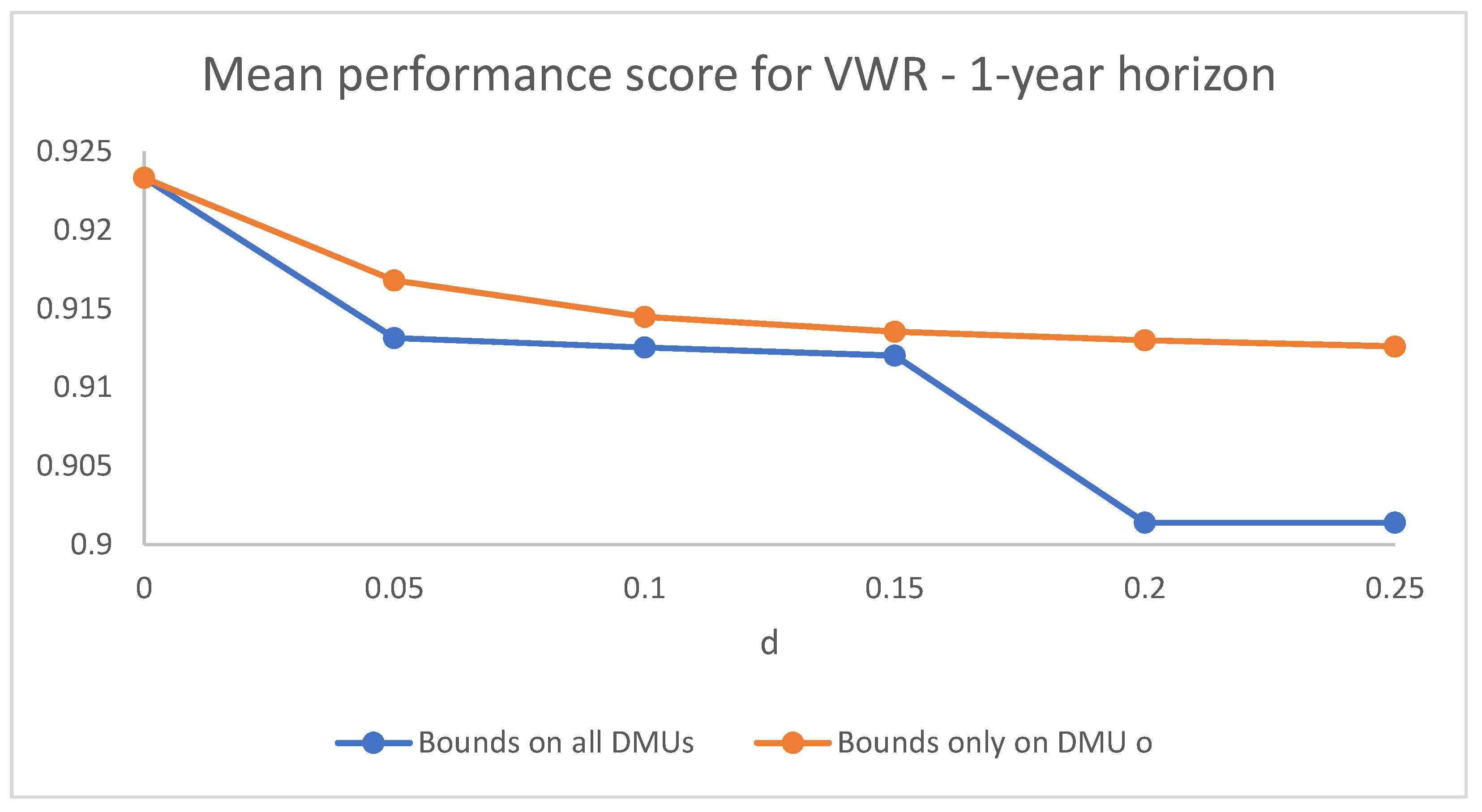
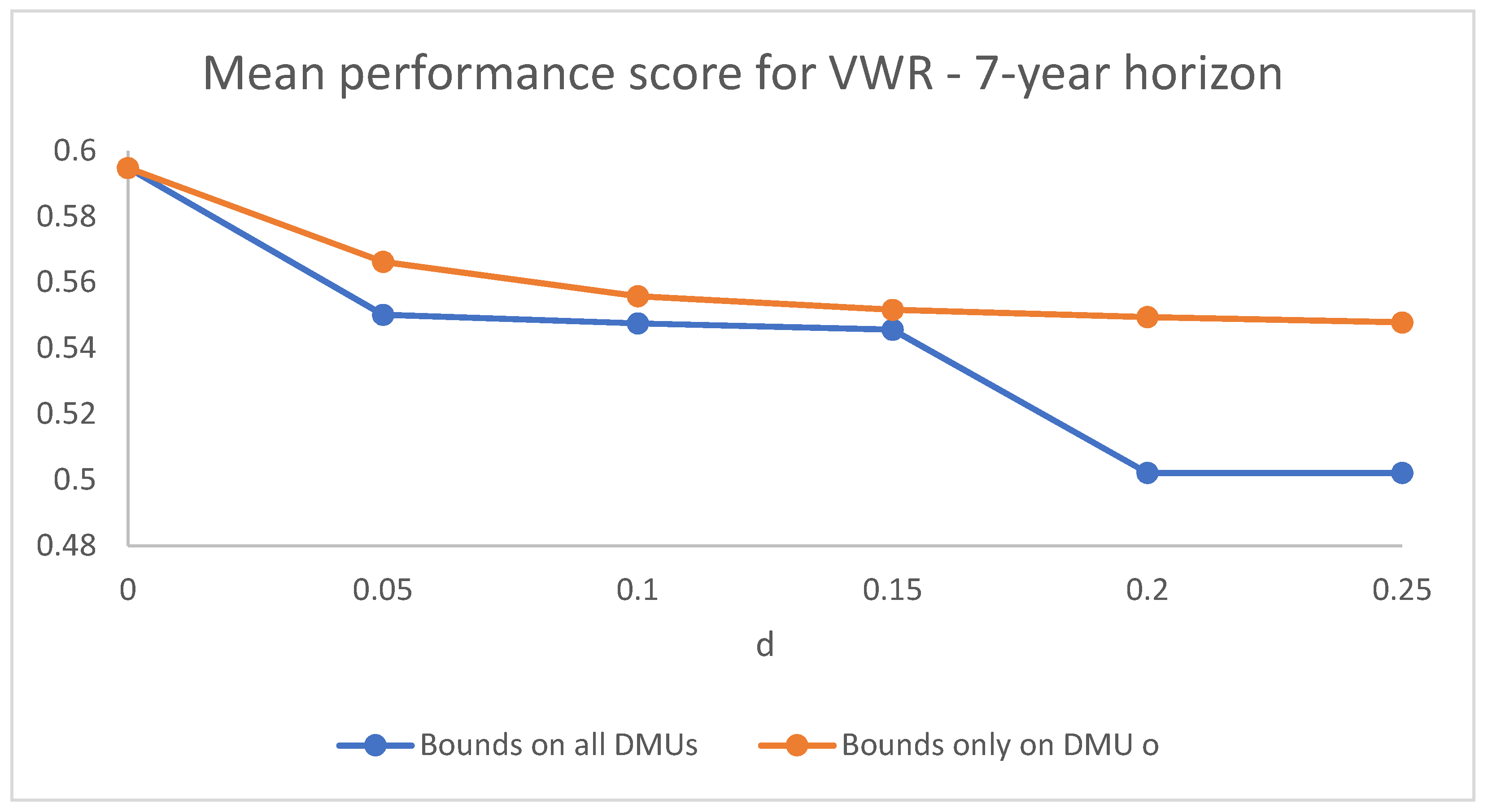
Figure 1 and Figure 2 compare the dynamics of the mean performance score in the cases of virtual weight restrictions set for all DMUs and of virtual weight restrictions with constraints on the target DMU as the bounds become more and more strict (as d increases) for $T=1$ and $T=7$, respectively. The case represented is that of symmetric bounds, but the dynamic behaviour in the asymmetric cases is analogous. The difference in the dynamics is appreciable mainly for the higher values of d.

7.4. Applying Assurance Region Weight Restrictions

In this subsection, we summarize the results of the analysis that regards the weight restrictions with assurance regions.

In order to investigate the results of the performance evaluation as the restrictions on the assurance regions become increasingly strict, we have computed the performance scores for different values of the lower bounds on the ratio between the input weights (let us recall that the upper bounds are redundant once the lower bounds are set, see Section 3.2).

More precisely, we have compared the results with respect to a parameter d which affects the value of the lower bounds, with $d\in [0,0.9]$. The case $d=0$ corresponds to the case without weight restrictions, while, as the value of d increases, the lower bounds on the assurance regions increase.

As with the virtual weight restrictions, we have considered three different cases: a symmetric case in which the bounds are the same for all input variables and two asymmetric cases in which the bounds for the initial payout K are different from the bounds of the risk measures $\beta$ and $DR$.

In the symmetric case, the lower bounds are calculated in the following way:

$$L_{i^{\prime }i}^X=\frac{d}{\frac{Mean(X_i)}{Mean(X_{i^{\prime }})}},$$

(104)

where $X_i$ represents the i-th input variable and the means are computed with respect to all mutual funds analyzed. By defining the lower bound $L_{i^{\prime }i}^X$ in this way, we “standardize” it, in a sense, with respect to the magnitude of the input variables, making it independent of the units of measurement chosen for the variables.

As for the asymmetric cases, in the one-year case, the bounds involving K are set so that the relevance of the initial payout is stressed when the holding period is short ($T=1$) while it is lessened in the seven-year case. In particular, the bounds involving K for $T=1$ are set as follows:

$$\begin{array}{cc}\hfill & L_{K\beta }^X=\frac{0.5d}{\frac{Mean(\beta )}{Mean(K)}}{L}_{K,DR}^X=\frac{0.5d}{\frac{Mean(DR)}{Mean(K)}},\hfill \end{array}$$

(105)

$$\begin{array}{cc}\hfill & L_{\beta K}^X=\frac{2d}{\frac{Mean(K)}{Mean(\beta )}}{L}_{DR,K}^X=\frac{2d}{\frac{Mean(K)}{Mean(DR)}},\hfill \end{array}$$

(106)

and the bounds involving K for $T=7$ are set as follows:

$$\begin{array}{cc}\hfill & L_{K\beta }^X=\frac{2d}{\frac{Mean(\beta )}{Mean(K)}}{L}_{K,DR}^X=\frac{2d}{\frac{Mean(DR)}{Mean(K)}},\hfill \end{array}$$

(107)

$$\begin{array}{cc}\hfill & L_{\beta K}^X=\frac{0.5d}{\frac{Mean(K)}{Mean(\beta )}}{L}_{DR,K}^X=\frac{0.5d}{\frac{Mean(K)}{Mean(DR)}}.\hfill \end{array}$$

(108)

The lower bounds imposed are summarized in

Table 10. Lower bounds considered for the assurance regions (AR) restrictions in the performance analysis of mutual funds for $d\in [0,0.9]$. The lower bounds are calculated dividing the values reported in the table by the ratio between the mean values of the variables.

Input Variables	K	$\mathit{\beta }$	$\mathbf{DR}$
Symmetric bounds
Initial payout K	1	d	d
$\beta$-coefficient	d	1	d
Downside risk $DR$	d	d	1
Asymmetric bounds—one-year holding period
Initial payout K	1	$0.5d$	$0.5d$
$\beta$-coefficient	$2d$	1	d
Downside risk $DR$	$2d$	d	1
Asymmetric bounds—seven-year holding period
Initial payout K	1	$2d$	$2d$
$\beta$-coefficient	$0.5d$	1	d
Downside risk $DR$	$0.5d$	d	1

, which shows the numerator of Formulas (104)–(108); the lower bounds for all pairs of input variables are calculated by dividing the values reported in the table by the ratio between the mean values of the variables, computed over all the mutual funds.

The main results of the analysis carried out are summarized in

Table 11. Main results for AR restrictions in the case of symmetric bounds and $T=1$. Summary statistics on the performance scores (minimum, mean and median values, standard deviation), number of efficient funds and mean absolute variation (divided by 2) of the ranking positions.

d	Minimum Score	Mean Score	Median Score	Std Dev of Score	Number of Efficient Funds	Mean Abs. Variation of Ranking
0.00	0.7690	0.9233	0.9193	0.0327	6	–
0.10	0.7601	0.9150	0.9126	0.0330	5	8.4119
0.20	0.7597	0.9136	0.9114	0.0327	5	9.7500
0.30	0.7593	0.9131	0.9111	0.0326	5	10.1122
0.40	0.7590	0.9127	0.9109	0.0326	5	10.3429
0.50	0.7587	0.9125	0.9107	0.0326	4	10.4679
0.60	0.7585	0.9124	0.9105	0.0326	4	10.5417
0.70	0.7582	0.9122	0.9103	0.0326	4	10.6298
0.80	0.7580	0.9121	0.9102	0.0326	4	10.6955
0.90	0.7579	0.9120	0.9100	0.0326	4	10.7372

,

Table 12. Main results for AR restrictions in the case of symmetric bounds and $T=7$. Summary statistics on the performance scores (minimum, mean and median values, standard deviation), number of efficient funds and mean absolute variation (divided by 2) of the ranking positions.

d	Minimum Score	Mean Score	Median Score	Std Dev of Score	Number of Efficient Funds	Mean Abs. Variation of Ranking
0.00	0.1583	0.5948	0.5635	0.1401	6	–
0.10	0.1464	0.5589	0.5325	0.1341	5	9.0929
0.20	0.1458	0.5522	0.5276	0.1310	4	10.5657
0.30	0.1453	0.5499	0.5271	0.1304	4	11.0208
0.40	0.1449	0.5486	0.5264	0.1301	4	11.2708
0.50	0.1446	0.5477	0.5256	0.1299	4	11.3766
0.60	0.1442	0.5471	0.5249	0.1297	4	11.4631
0.70	0.1439	0.5465	0.5245	0.1296	4	11.5737
0.80	0.1437	0.5461	0.5242	0.1295	4	11.6362
0.90	0.1435	0.5458	0.5239	0.1294	4	11.6779

,

Table 13. Main results for AR restrictions in the case of asymmetric bounds and $T=1$. Summary statistics on the performance scores (minimum, mean and median values, standard deviation), number of efficient funds and mean absolute variation (divided by 2) of the ranking positions.

d	Minimum Score	Mean Score	Median Score	Std Dev of Score	Number of Efficient Funds	Mean Abs. Variation of Ranking
0.00	0.7690	0.9233	0.9193	0.0327	6	–
0.10	0.7614	0.9170	0.9143	0.0330	6	6.3045
0.20	0.7600	0.9150	0.9120	0.0330	5	8.4183
0.30	0.7596	0.9140	0.9114	0.0328	5	9.3077
0.40	0.7593	0.9134	0.9110	0.0327	5	9.7468
0.50	0.7590	0.9131	0.9108	0.0327	5	9.9840
0.60	0.7588	0.9129	0.9106	0.0326	5	10.1378
0.70	0.7586	0.9127	0.9105	0.0326	5	10.2708
0.80	0.7583	0.9125	0.9104	0.0326	4	10.3670
0.90	0.7582	0.9124	0.9104	0.0326	4	10.4551

and

Table 14. Main results for AR restrictions in the case of asymmetric bounds and $T=7$. Summary statistics on the performance scores (minimum, mean and median values, standard deviation), number of efficient funds and mean absolute variation (divided by 2) of the ranking positions.

d	Minimum Score	Mean Score	Median Score	Std Dev of Score	Number of Efficient Funds	Mean Abs. Variation of Ranking
0.00	0.1583	0.5948	0.5635	0.1401	6	–
0.10	0.1461	0.5525	0.5281	0.1311	4	10.5978
0.20	0.1456	0.5493	0.5271	0.1301	4	11.2772
0.30	0.1451	0.5480	0.5255	0.1299	4	11.4744
0.40	0.1447	0.5471	0.5248	0.1297	4	11.5689
0.50	0.1443	0.5466	0.5244	0.1296	4	11.6490
0.60	0.1440	0.5461	0.5241	0.1295	4	11.7324
0.70	0.1437	0.5457	0.5237	0.1295	4	11.7869
0.80	0.1435	0.5454	0.5234	0.1294	4	11.8093
0.90	0.1433	0.5451	0.5232	0.1294	4	11.8189

, for the symmetric and asymmetric bounds and for $T=1$ and $T=7$. In general, the behaviour of both the performance scores and the differences in the rankings are similar to that observed for the virtual weight restrictions.

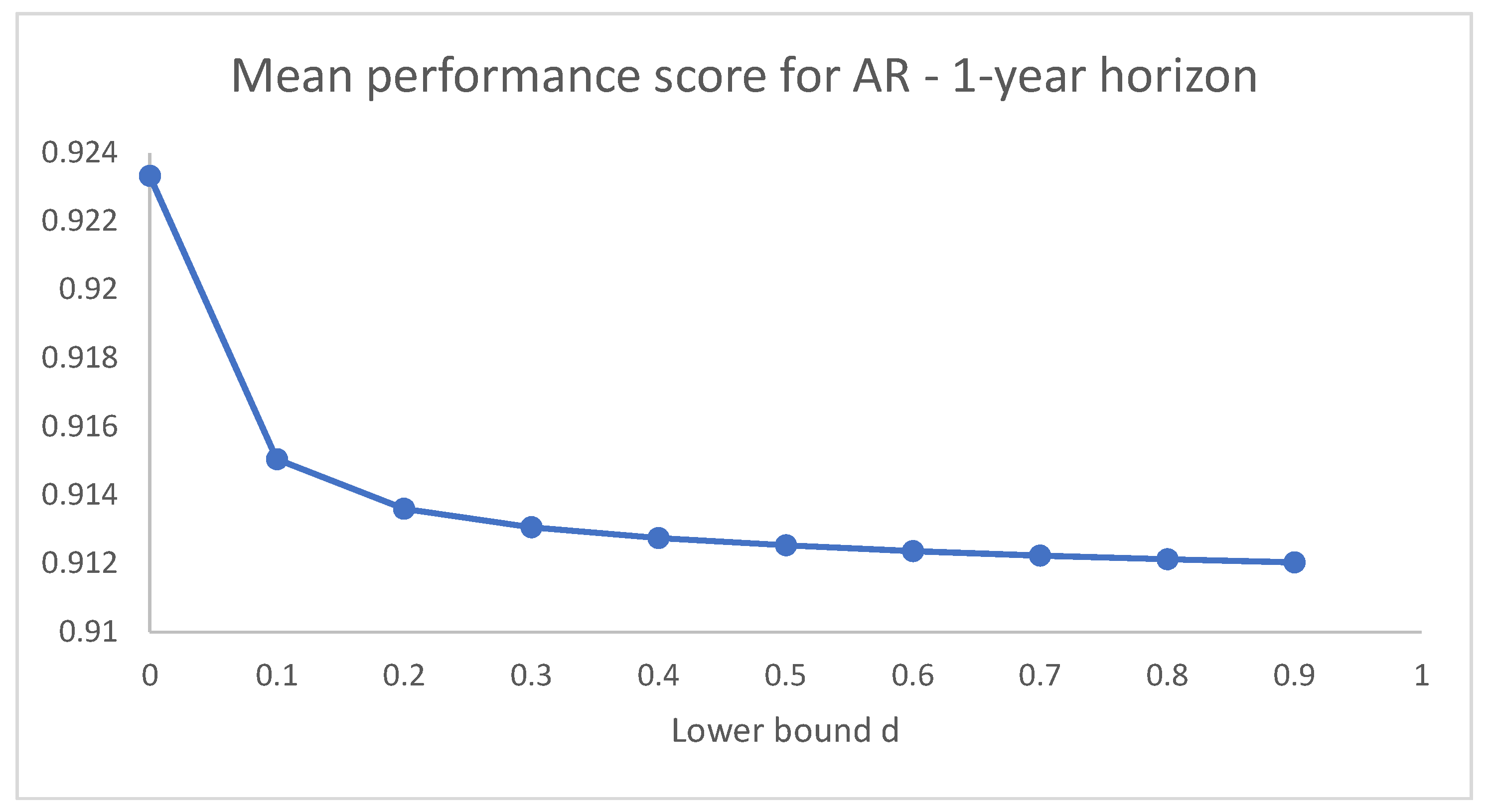
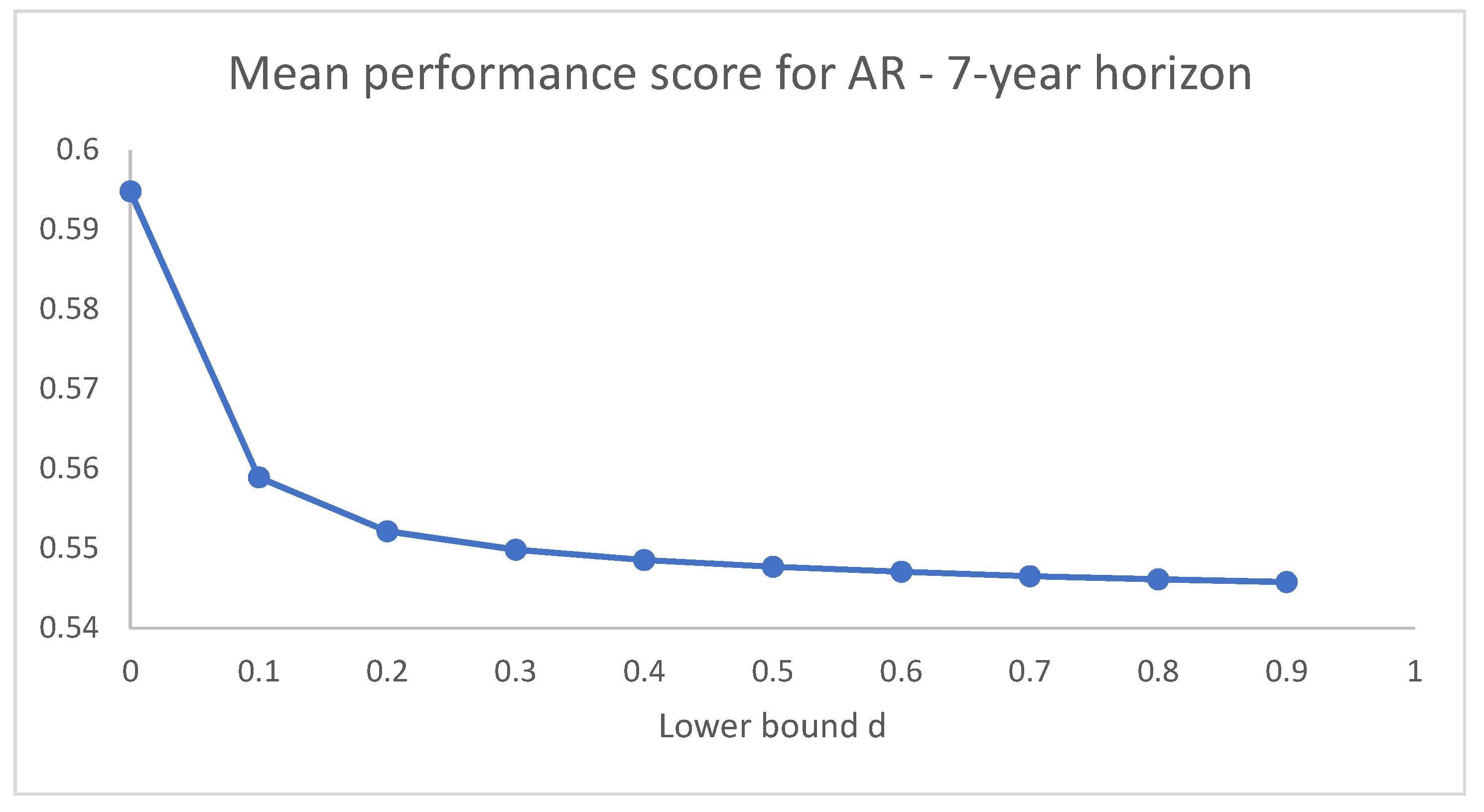
Figure 3 and Figure 4 illustrate the dynamics of the mean performance score for the short and long holding periods considered ($T=1$ and $T=7$), respectively. As observed for the results obtained with VW restrictions, we may notice that the behaviour of the dynamics of the mean performance scores is similar, although the mean values are rather different since the values of the scores in the seven-year case are more dispersed than in the one-year case.

8. Conclusions

The introduction of weight restrictions in DEA models which are adopted to evaluate the performance of mutual funds may be important to ensure that no relevant variables are neglected in the assessment of the fund performance.

In this contribution, we provide a unified matrix representation for three types of weight restrictions: virtual weight restrictions with constraints on all funds, virtual weight restrictions with constraints only on the target fund and restrictions with assurance regions.

In addition, in order to investigate the effect of the introduction of these restrictions on the DEA models and undertake a detailed sensitivity analysis, we carry out an empirical study on a large number of European mutual funds.

The experimental application carried out aims both to investigate the effects on the performance scores of the three different kinds of weight restrictions considered, and to analyze the behaviour of the fund performance scores as the restrictions on the weights become increasingly strict.

In summary, the results show that, by setting restrictions on the weights into a DEA model for mutual funds, the performance scores and the fund ranking change in a sensible manner but not drastically. The mean performance score and the number of efficient funds diminish as the bounds become stricter and this effect is more pronounced in the case of virtual weight restrictions with constraints on all funds.

Let us point out that in this paper we have focused on a general DEA model with variable returns to scale and an output orientation; however, it is possible to derive a similar matrix representation also for input oriented models and for models exhibiting constant returns to scale.