Some Notes about Inference for the Lognormal Diffusion Process with Exogenous Factors

Abstract

Different versions of the lognormal diffusion process with exogenous factors have been used in recent years to model and study the behavior of phenomena following a given growth curve. In each case considered, the estimation of the model has been addressed, generally by maximum likelihood (ML), as has been the study of several characteristics associated with the type of curve considered. For this process, a unified version of the ML estimation problem is presented, including how to obtain estimation errors and asymptotic confidence intervals for parametric functions when no explicit expression is available for the estimators of the parameters of the model. The Gompertz-type diffusion process is used here to illustrate the application of the methodology.

1. Introduction

The lognormal diffusion process has been widely used as a probabilistic model in several scientific fields in which the variable under consideration exhibits an exponential trend. Originally, the lognormal diffusion process was mainly applied to modeling dynamic variables in the field of economy and finance. Important contributions have been made in this direction by Cox and Ross [1], Markus and Shaked [2], and Merton [3], showing the theoretical and practical importance of the process in that environment. For example, this process is associated with the Black and Scholes model [4] and appears in later extensions as terminal swap-rate models (Hunt and Kennedy [5], Lamberton and Lapeyre [6]).

In 1972, Tintner and Sengupta [7] introduced a modification of the process by including a linear combination of time functions in the infinitesimal mean of the process. The motivation for this was the introduction of external influences on the interest variable (endogenous variable), influences that could contribute to a better explanation of the phenomenon under study. For this reason, these time functions are known as exogenous factors, whose time behavior is assumed to be known or partially known. By using these time functions we can model situations wherein the observed trend shows deviations from the theoretical shape of the trend during certain time intervals, and can therefore use them to help describe the evolution of the process. Furthermore, a suitable choice of the exogenous factors can contribute to the external control of the process for forecasting purposes. Note that the methodology derived from the inclusion of exogenous factors has been applied to several contexts other than the lognormal process (see, for example, Buonocore et al. [8]).

The lognormal diffusion process with exogenous factors has been widely studied in relation to some aspects of inference and first-passage times. It has been applied to the modeling of time variables in several fields (see, for example [9,10]). On occasion, the endogenous variable itself helps identify the exogenous factors. However, there are situations in which external variables to the process that have an influence on the system are not available, or situations in which their functional expressions are unknown. In such cases, Gutiérrez et al. [11] suggested approaching the exogenous factors by means of polynomial functions.

The ability to control the endogenous variable using exogenous factors makes this process particularly useful for forecasting purposes. Some of its main features, such as the mean, mode and quantile functions (that can be expressed as parametric functions of the parameters of the process), can be used for prediction purposes. Therefore, the inference of these functions has been the subject of considerable study, both from the perspective of point estimation and of estimation by confidence intervals. With respect to the former, in [10] a more general study was carried out to obtain maximum likelihood (ML) estimators. In that case, the exact distribution of the estimators was found, and then used to obtain the uniformly minimum variance unbiased (UMVU) estimators. In addition, expressions for the relative efficiency of ML estimators, with respect to UMVU estimators, were obtained. This last study was extended for a class of parametric functions which include the mean and mode functions (together with their conditional versions) as special cases. Concerning estimation by confidence bands, in this paper the authors extended the results obtained by Land [12] on exact confidence intervals for the mean of a lognormal distribution, thus obtaining confidence bands for the mean and mode functions of the lognormal process with exogenous factors and expressing these functions in a more general form.

In most of the works cited, inference has been approached from the ML point of view, considering discrete sampling of the trajectories. To this end, it is essential to have the exact form of the transition density functions from which the likelihood function associated with the sample is constructed. However, alternatives are available for a range of situations. For example, approximating the transition density function using Euler-type schemes derived from the discretization of the stochastic differential equation that models the behavior of the phenomenon under study (sometimes this approach is known as naive ML approach). Other possible alternatives to ML are those derived, for example, from the use of the concept of estimating functions (Bibby et al. [13]) and the generalized method of moments (Hansen [14]). Fuchs in [15] presents a good review of these and other procedures. The Bayesian approach is also present in the study of diffusion processes, as suggested by Tang and Heron in [16].

On the other hand, considering particular choices of the time functions that define the exogenous factors has enabled researchers to define diffusion processes associated to alternative expressions of already-known growth curves. Along these lines, we may cite a Gompertz-type process [17] (applied to the study of rabbit growth), a generalized Von Bertalanffy diffusion process [18] (with an application to the growth of fish species), a logistic-type process [19] (applied to the growth of a microorganism culture), and a Richards-type diffusion process [20]. In [21], a joint analysis of the procedure for obtaining these processes is shown. More recently, Da Luz-Sant’Ana et al. [22] have established, following a similar methodology, a Hubbert diffusion process for studying oil production, while Barrera et al. [23] introduced a process linked to the hyperbolastic type-I curve and applied it in the context of the quantitative polymerase chain reaction (qPCR) technique.

In these last cases, obtaining the ML estimators was a rather laborious task. In fact, the resulting system of equations is exceedingly complex and does not have an explicit solution, and numerical procedures must be employed instead, with the subsequent problem of finding initial solutions (see, for instance [18,19,22]). However, it is impossible to carry out a general study of the system of equations in order to check the conditions of convergence of the chosen numerical method, since it is dependent on sample data. One alternative is then to use stochastic optimization procedures like simulated annealing, variable neighborhood search, and the firefly algorithm [20,23,24]. In any case, the exact distribution of the estimators cannot be obtained. Recently, the asymptotic distribution of the MLestimators and delta method have been used in order to obtain estimation errors, as well as confidence intervals, for the parameters and parametric functions in the context of the Hubbert diffusion model [25].

The main objective of this paper is to provide a unified view of the estimation problem by means of discrete sampling of trajectories, and to cover all the diffusion processes mentioned above. To this end, we will consider the generic expression of the lognormal diffusion process with exogenous factors. In Section 2, a brief summary of the main characteristics of the process is presented. Section 3 and Section 4 address the problem of estimation by ML by using discrete sampling. In Section 3, the distribution of the sample is obtained, while in Section 4 the generic form adopted by the system of likelihood equations is derived in terms of the exogenous factor included in the model. Section 5 deals with obtaining the asymptotic distribution of the estimators, after calculating the Fisher information matrix, for which the results of Section 3 are fundamental. Finally, and as an application of the previous developments, Section 6 deals with the particular case of the Gompertz-type process introduced in [17].

2. The Lognormal Diffusion Process With Exogenous Factors

Let $I=[t_0,+\infty )$ be a real interval ($t_0\ge 0$), $\Theta \subseteq {\mathbb{R}}^k$ an open set, and $h_{\mathit{\theta }}(t)$ a continuous, bounded and differentiable function on I depending on $\mathit{\theta }\in \Theta$.

The univariate lognormal diffusion process with exogenous factors is a diffusion process $\{X(t);t\in I\}$, taking values on ${\mathbb{R}}^{+}$, with infinitesimal moments

$$\begin{array}{c}{A}_1(x,t)=h_{\mathit{\theta }}(t)x\hfill \\ A_2(x)={\sigma }^2{x}^2,\sigma >0\hfill \end{array}$$

(1)

and with a lognormal or degenerate initial distribution. This process is the solution to the stochastic differential equation

$$dX(t)=h_{\mathit{\theta }}(t)X(t)dt+\sigma X(t)dW(t),X(t_0)=X_0,$$

where $W(t)$ is a standard Wiener process independent on $X_0=X(t_0)$, $t\ge t_0$, being this solution

$$X(t)=X_0\exp \left(H_{\mathit{\xi }}(t_0,t)+\sigma (W(t)-W(t_0))\right),t\ge t_0$$

with

$$H_{\mathit{\xi }}(t_0,t)={\int }_{t_0}^t{h}_{\mathit{\theta }}(u)du-\frac{{\sigma }^2}{2}(t-t_0),\mathit{\xi }={({\mathit{\theta }}^T,{\sigma }^2)}^T.$$

An explanation of the main features of the process can be found in [21], where the authors carried out a detailed theoretical analysis. As regards the distribution of the process, if $X_0$ is distributed according to a lognormal distribution ${\Lambda }_1\left[{\mu }_0;{\sigma }_0^2\right]$, or $X_0$ is a degenerate variable ($P[X_0=x_0]=1$), all the finite-dimensional distributions of the process are lognormal. Concretely, $\forall n\in \mathbb{N}$ and $t_1<\cdots <t_n$, vector ${(X(t_1),\dots ,X(t_n))}^T$ has a n-dimensional lognormal distribution ${\Lambda }_n[\mathit{\epsilon },\mathbf{\Sigma }]$, where the components of vector $\mathit{\epsilon }$ and matrix $\mathbf{\Sigma }$ are

$${\epsilon }_i={\mu }_0+H_{\mathit{\xi }}(t_0,t_i),i=1,\dots ,n$$

and

$${\sigma }_{ij}={\sigma }_0^2+{\sigma }^2(\min (t_i,t_j)-t_0),i,j=1,\dots ,n,$$

respectively. The transition probability density function can be obtained from the distribution of ${(X(s),X(t))}^T$, $s<t$, being

$$f(x,t|y,s)=\frac{1}{x\sqrt{2\pi {\sigma }^2(t-s)}}\exp \left(-\frac{{\left[\ln (x/y)-H_{\mathit{\xi }}(s,t)\right]}^2}{2{\sigma }^2(t-s)}\right),$$

(2)

that is, $X(t)|X(s)=y$ follows a lognormal distribution

$$X(t)\mid X(s)=y⇝{\Lambda }_1\left(\ln y+H_{\mathit{\xi }}(s,t),{\sigma }^2(t-s)\right),s<t.$$

From the previous distributions, one can obtain the characteristics most commonly employed for practical fitting and forecasting purposes. These characteristics can be expressed jointly as

$$G_{\mathit{\xi }}^{\mathit{\lambda }}(t|y,\tau )=M_{\mathit{\xi }}{(t|y,\tau )}^{{\lambda }_1}\exp \left({\lambda }_2{\left({\lambda }_3{\sigma }_0^2+{\sigma }^2(t-\tau )\right)}^{{\lambda }_4}\right),$$

(3)

with $\mathit{\lambda }={({\lambda }_1,{\lambda }_2,{\lambda }_3,{\lambda }_4)}^T$ and where $M_{\mathit{\xi }}(t|y,\tau )=\exp \left(y+H_{\xi }(\tau ,t)\right)$.

Table 1. Values used to obtain the n-th moment and the mode and quantile functions from $G_{\mathit{\xi }}^{\mathit{\lambda }}(t|z,\tau )$. $z_{\alpha }$ is the $\alpha$-quantile of a standard normal distribution.

Function	Expression	z	$\mathit{\tau }$	$\mathit{\lambda }$
n-th moment	$E[X{(t)}^n]$	${\mu }_0$	$t_0$	${(n,n^2/2,1,1)}^T$
n-th conditional moment	$E[X{(t)}^n|X(s)=y]$	$\ln y$	s	${(n,n^2/2,0,1)}^T$
mode	$Mode[X(t)]$	${\mu }_0$	$t_0$	${(1,-1,1,1)}^T$
conditional mode	$Mode[X(t)|X(s)=y]$	$\ln y$	s	${(1,-1,0,1)}^T$
$\alpha$-quantile	$C_{\alpha }[X(t)]$	${\mu }_0$	$t_0$	${(1,z_{\alpha },1,1/2)}^T$
$\alpha$-conditional quantile	$C_{\alpha }[X(t)|X(s)=y]$	$\ln y$	s	${(1,z_{\alpha },0,1/2)}^T$

includes some of these characteristics (the $n-$th moment, and the mode and quantile functions as well as their conditional versions) according to the values of $\mathit{\lambda }$, $\tau$ and y.

3. Joint Distribution of $\mathit{d}$ Sample-Paths of the Process

Let us consider a discrete sampling of the process, based on d sample paths, at times $t_{ij}$, $(i=1,\dots ,d,j=1,\dots ,n_i)$ with $t_{i1}$ = $t_0$, $i=1,\dots ,d$. Denote by $\mathbf{X}={\left({\mathbf{X}}_1^T|\cdots |{\mathbf{X}}_d^T\right)}^T$ the vector containing the random variables of the sample, where ${\mathbf{X}}_i^T$ includes the variables of the i-th sample-path, that is ${\mathbf{X}}_i={(X(t_{i1}),\dots ,X(t_{i,n_i}))}^T$, $i=1,\dots ,d$.

From Equation (2), and if the distribution of $X(t_1)$ is assumed lognormal ${\Lambda }_1({\mu }_1,{\sigma }_1^2)$, the probability density function of $\mathbf{X}$ is

$$\begin{array}{cc}\hfill f_{\mathbf{X}}(\mathbf{x})& {\displaystyle ={\displaystyle \prod _{i=1}^d}\frac{\exp \left(-\frac{{[\ln x_{i1}-{\mu }_1]}^2}{2{\sigma }_1^2}\right)}{x_{i1}{\sigma }_1\sqrt{2\pi }}{\displaystyle \prod _{j=1}^{n_i-1}}\frac{\exp \left(-\frac{{\left[\ln \left(x_{i,j+1}/x_{ij}\right)-m_{\mathit{\xi }}^{i,j,j+1}\right]}^2}{2{\sigma }^2{\Delta }_i^{j+1,j}}\right)}{x_{ij}\sigma \sqrt{2\pi {\Delta }_i^{j+1,j}}}}\hfill \end{array}$$

where $m_{\mathit{\xi }}^{i,j+1,j}=H_{\mathit{\xi }}(t_{ij},t_{i,j+1})$ and ${\Delta }_i^{j+1,j}=t_{i,j+1}-t_{ij}.$

Now, we consider vector $\mathbf{V}={\left[{\mathbf{V}}_0^T|{\mathbf{V}}_1^T|\cdots |{\mathbf{V}}_d^T\right]}^T={\left[{\mathbf{V}}_0^T|{\mathbf{V}}_{(1)}^T\right]}^T$, built from $\mathbf{X}$ by means of the following change of variables:

$$\begin{array}{cc}\hfill V_{0i}& =X_{i1},i=1,\dots ,d\hfill \\ \hfill V_{ij}& ={({\Delta }_i^{j+1,j})}^{-1/2}\ln \frac{X_{i,j+1}}{X_{ij}},i=1,\dots ,d;j=1,\dots ,n_i-1.\hfill \end{array}$$

(4)

Taking into account this change of variables, the density of $\mathbf{V}$ becomes

$${\displaystyle f_{\mathbf{V}}(\mathbf{v})=\frac{\exp \left(-\frac{1}{2{\sigma }_1^2}{(\ln {\mathbf{v}}_0-{\mu }_1{\mathbf{1}}_d)}^T(\ln {\mathbf{v}}_0-{\mu }_1{\mathbf{1}}_d)\right)}{{\displaystyle \prod _{i=1}^d{v}_{0i}{\left(2\pi {\sigma }_1^2\right)}^{\frac{d}{2}}}}\frac{\exp \left(-\frac{1}{2{\sigma }^2}{\left({\mathbf{v}}_{(1)}-{\mathit{\gamma }}^{\mathit{\xi }}\right)}^T\left({\mathbf{v}}_{(1)}-{\mathit{\gamma }}^{\mathit{\xi }}\right)\right)}{{\left(2\pi {\sigma }^2\right)}^{\frac{n}{2}}}}$$

(5)

with $\ln {\mathbf{v}}_0={(\ln v_{01},\dots ,\ln v_{0d})}^T$, $n={\sum }_{i=1}^d(n_i-1)$. Here, ${\mathbf{1}}_d$ represents the d-dimensional vector whose components are all equal to one, while ${\mathit{\gamma }}^{\mathit{\xi }}$ is a vector of dimension n with components ${\gamma }_{ij}^{\mathit{\xi }}={({\Delta }_i^{j+1,j})}^{-1/2}{m}_{\xi }^{i,j,j+1}$, $i=1,\dots ,d;j=1,\dots ,n_i-1$.

From Equation (5) it is deduced that:

• ${\mathbf{V}}_0$ and ${\mathbf{V}}_{(1)}$ are independents,
• the distribution of ${\mathbf{V}}_0$ is lognormal ${\Lambda }_d\left[{\mu }_1{\mathbf{1}}_d;{\sigma }_1^2{\mathbf{I}}_d\right]$,
• ${\mathbf{V}}_{(1)}$ is distributed as an n-variate normal distribution $N_n\left[{\mathit{\gamma }}^{\mathit{\xi }};{\sigma }^2{\mathbf{I}}_n\right]$,

being ${\mathbf{I}}_d$ and ${\mathbf{I}}_n$ the identity matrices of order d and n, respectively.

4. Maximum Likelihood Estimation of the Parameters of the Process

Consider a discrete sample of the process in the sense described in the previous section, including the transformation of it given by Equation (4). Denote by $\mathit{\eta }={({\mu }_1,{\sigma }_1^2)}^T$ and suppose that $\mathit{\eta }$ and $\mathit{\xi }$ are functionally independent. Then, for a fixed value $\mathbf{v}$ of the sample, the log-likelihood function is

$$\begin{array}{cc}\hfill L_{\mathbf{v}}(\mathit{\eta },\mathit{\xi })& =-\frac{(n+d)\ln (2\pi )}{2}-\frac{d\ln {\sigma }_1^2}{2}-{\displaystyle \sum _{i=1}^d}\ln v_{0i}-\frac{{\displaystyle \sum _{i=1}^d{\left[\ln v_{0i}-{\mu }_1\right]}^2}}{2{\sigma }_1^2}-\frac{n \ln {\sigma }^2}{2}-\frac{Z_1+{\Phi }_{\mathit{\xi }}-2{\Gamma }_{\mathit{\xi }}}{2{\sigma }^2}\hfill \end{array}$$

(6)

where

$${\displaystyle Z_1=\sum _{i=1}^d\sum _{j=1}^{n_i-1}{v}_{ij}^2,{\Phi }_{\mathit{\xi }}=\sum _{i=1}^d\sum _{j=1}^{n_i-1}\frac{{\left(m_{\mathit{\xi }}^{i,j+1,j}\right)}^2}{{\Delta }_i^{j+1,j}},{\Gamma }_{\mathit{\xi }}=\sum _{i=1}^d\sum _{j=1}^{n_i-1}\frac{v_{ij}{m}_{\mathit{\xi }}^{i,j+1,j}}{{({\Delta }_i^{j+1,j})}^{1/2}}.}$$

Taking into account Equation (6), and since $\mathit{\eta }$ and $\mathit{\xi }$ are functionally independent, the ML estimation of $\mathit{\eta }$ is obtained from the system of equations (Given a function $f:{\mathbb{R}}^k\to \mathbb{R}$, $\frac{\partial f}{\partial {\mathbf{x}}^T}=\left(\frac{\partial f}{\partial x_1},\dots ,\frac{\partial f}{\partial x_k}\right)$. Notation $\frac{\partial f}{\partial {\mathbf{x}}^T}$ indicates that the result is a row vector).

$$\frac{\partial L_{\mathbf{v}}(\mathit{\eta },\mathit{\xi })}{\partial {\mathit{\eta }}^T}=\left(\frac{\partial L_{\mathbf{v}}(\mathit{\eta },\mathit{\xi })}{\partial {\mu }_1},\frac{\partial L_{\mathbf{v}}(\mathit{\eta },\mathit{\xi })}{\partial {\mathit{\sigma }}_1^2}\right)=\mathbf{0}$$

resulting in

$${\displaystyle {\widehat{\mu }}_1=\frac{1}{d}\sum _{i=1}^d\ln v_{0i}\mathrm{and}{\widehat{\sigma }}_1^2=\frac{1}{d}\sum _{i=1}^d{(\ln v_{0i}-{\widehat{\mu }}_1)}^2.}$$

On the other hand, by denoting

$$\begin{array}{c}{\Omega }_{\mathit{\xi }}=\frac{1}{2}\frac{\partial {\Phi }_{\mathit{\xi }}}{\partial {\mathit{\theta }}^T}={\displaystyle \sum _{i=1}^d}{\displaystyle \sum _{j=1}^{n_i-1}}\frac{m_{\mathit{\xi }}^{i,j+1,j}}{{\Delta }_i^{j+1,j}}\frac{\partial m_{\mathit{\xi }}^{i,j+1,j}}{\partial {\mathit{\theta }}^T},{\Psi }_{\mathit{\theta }}=\frac{1}{2}\frac{\partial {\Gamma }_{\mathit{\xi }}}{\partial {\mathit{\theta }}^T}={\displaystyle \sum _{i=1}^d}{\displaystyle \sum _{j=1}^{n_i-1}}\frac{v_{ij}}{{({\Delta }_i^{j+1,j})}^{1/2}}\frac{\partial m_{\mathit{\xi }}^{i,j+1,j}}{\partial {\mathit{\theta }}^T}\\ {{\rm Y}}_{\mathit{\xi }}=-\frac{\partial {\Phi }_{\mathit{\xi }}}{\partial {\sigma }^2}={\displaystyle \sum _{i=1}^d}{m}_{\mathit{\xi }}^{i,n_i,1},Z_2=-2\frac{\partial {\Gamma }_{\mathit{\xi }}}{\partial {\sigma }^2}={\displaystyle \sum _{i=1}^d}{\displaystyle \sum _{j=1}^{n_i-1}}{v}_{ij}{({\Delta }_i^{j+1,j})}^{1/2}\end{array}$$

(7)

we have

$$\begin{array}{cc}\hfill \frac{\partial L_{\mathbf{v}}(\mathit{\eta },\mathit{\xi })}{\partial {\mathit{\theta }}^T}& =\frac{1}{{\sigma }^2}\left[{\Psi }_{\mathit{\theta }}-{\Omega }_{\mathit{\xi }}\right]\hfill \\ \hfill \frac{\partial L_{\mathbf{v}}(\mathit{\eta },\mathit{\xi })}{\partial {\sigma }^2}& =-\frac{n}{2{\sigma }^2}+\frac{Z_1+{\Phi }_{\mathit{\xi }}-2{\Gamma }_{\mathit{\xi }}}{2{\sigma }^4}-\frac{Z_2-{{\rm Y}}_{\mathit{\xi }}}{2{\sigma }^2}.\hfill \end{array}$$

Thus, the ML estimation of $\mathit{\xi }$ is obtained as the solution of the following system of $k+1$ equations:

$$\begin{array}{c}{\Psi }_{\mathit{\theta }}-{\Omega }_{\mathit{\xi }}=0\hfill \end{array}$$

(8)

$$\begin{array}{c}{Z}_1+{\Phi }_{\mathit{\xi }}-2{\Gamma }_{\mathit{\xi }}-{\sigma }^2{Z}_2+{\sigma }^2{{\rm Y}}_{\mathit{\xi }}=n{\sigma }^2\hfill \end{array}$$

(9)

In the case where $h_{\mathit{\theta }}$ is a linear function in $\mathit{\theta }$, it is possible to determine an explicit solution for this system of equations (see [10,26]). In other cases, the existence of a closed-form solution can not be guaranteed, and it is therefore necessary to use numerical procedures for its resolution. The fact that these methods require initial solutions has motivated the construction of ad hoc procedures which depend on the process derived according to the function $h_{\mathit{\theta }}$ considered (see [18,19,22]). However, it is impossible to carry out a general study of the system of equations in order to check the conditions of convergence of the chosen numerical method, since the system is dependent on sample data and this may lead to unforeseeable behavior. One alternative would be using stochastic optimization procedures like simulated annealing, variable neighborhood search and the firefly algorithm. These algorithms are often more appropriate than classical numerical methods since they impose fewer restrictions on the space of solutions and on the analytical properties of the function to be optimized. Some examples of the application of these procedures in the context of diffusion processes can be seen in [19,21,23,25].

5. Distribution of the ML Estimators of the Parameters and Related Parametric Functions

In this section we will discuss some aspects related to the distribution of the estimators of the parameters of the model, and their repercussions in the corresponding distributions of parametric functions, which can be of interest for several applications.

With regard to the distribution of the estimators of $\mathit{\eta }$, it is immediate to verify that

$$\widehat{{\mu }_1}⇝N_1[{\mu }_1;{\sigma }_1^2/d]\mathrm{and}\frac{d\widehat{{\sigma }_1^2}}{{\sigma }_1^2}⇝{\chi }_{d-1}^2.$$

If $h_{\mathit{\theta }}$ is linear, it is then possible to calculate exact distributions associated with the estimators of $\mathit{\xi }$, which allows us to establish confidence regions for the parameters as well as UMVU estimators and confidence intervals for linear combinations of $\mathit{\theta }$ and ${\sigma }^2$ (see [10,26]). However, in the non-linear case, the fact that an explicit expression for the estimators of $\mathit{\xi }$ is not always readily available precludes obtaining, in general, exact distributions for them. In that case, asymptotic distributions can be used instead. In fact, on the basis of the properties of the ML estimators, it is known that $\widehat{\mathit{\xi }}$ is asymptotically distributed as a normal distribution with mean $\mathit{\xi }$ and covariance matrix $I{(\mathit{\xi })}^{-1}$, where $I(\xi )$ is the Fisher’s information matrix associated with the full sample (in this case, ignoring the data of the initial distribution).

First we calculate the associated Hessian matrix: (we have adopted the usual expression for the Hessian matrix of $f:{\mathbb{R}}^k\to \mathbb{R}$ using vectorial notation, that is ${\displaystyle \frac{{\partial }^{2}f}{\partial \mathbf{x}\partial {\mathbf{x}}^T}}$).

$$\begin{array}{cc}\hfill H(\mathit{\xi })& =\frac{{\partial }^2{L}_{\mathbf{v}}(\mathit{\eta },\mathit{\xi })}{\partial \mathit{\xi }\partial {\mathit{\xi }}^T}=\left(\begin{array}{cc}{\displaystyle \frac{{\partial }^2{L}_{\mathbf{v}}(\mathit{\eta },\mathit{\xi })}{\partial \mathit{\theta }\partial {\mathit{\theta }}^T}}& {\left({\displaystyle \frac{{\partial }^2{L}_{\mathbf{v}}(\mathit{\eta },\mathit{\xi })}{\partial {\sigma }^2\partial {\mathit{\theta }}^T}}\right)}^T\\ {\displaystyle \frac{{\partial }^2{L}_{\mathbf{v}}(\mathit{\eta },\mathit{\xi })}{\partial {\sigma }^2\partial {\mathit{\theta }}^T}}& {\displaystyle \frac{{\partial }^2{L}_{\mathbf{v}}(\mathit{\eta },\mathit{\xi })}{\partial {({\sigma }^2)}^2}}\end{array}\right)\hfill \\ & =\frac{1}{{\sigma }^2}\left(\begin{array}{cc}{\Pi }_{\mathit{\xi }}-{\Xi }_{\mathit{\xi }}& {\displaystyle -\frac{1}{{\sigma }^2}\left[{\Psi }_{\mathit{\theta }}^T-{\Omega }_{\mathit{\xi }}^T\right]+\frac{1}{2}{\left(\frac{\partial {{\rm Y}}_{\xi }}{\partial {\mathit{\theta }}^T}\right)}^T}\\ {\displaystyle -\frac{1}{{\sigma }^2}\left[{\Psi }_{\mathit{\theta }}-{\Omega }_{\mathit{\xi }}\right]+\frac{1}{2}\frac{\partial {{\rm Y}}_{\xi }}{\partial {\mathit{\theta }}^T}}& {\displaystyle \frac{n}{2{\sigma }^2}-\frac{Z_1+{\Phi }_{\mathit{\xi }}-2{\Gamma }_{\mathit{\xi }}}{{\sigma }^4}+\frac{Z_2-{{\rm Y}}_{\mathit{\xi }}}{{\sigma }^2}-\frac{Z_3}{4}}\end{array}\right)\hfill \end{array}$$

where

$${\displaystyle {\Pi }_{\mathit{\xi }}=\sum _{i=1}^d\sum _{j=1}^{n_i-1}\frac{{\partial }^2{m}_{\mathit{\xi }}^{i,j+1,j}}{\partial \mathit{\theta }\partial {\mathit{\theta }}^T}{({\Delta }_i^{j+1,j})}^{-1/2}\left(v_{ij}-{({\Delta }_i^{j+1,j})}^{-1/2}{m}_{\mathit{\xi }}^{i,j+1,j}\right)}$$

and

$${\displaystyle {\Xi }_{\mathit{\xi }}=\sum _{i=1}^d\sum _{j=1}^{n_i-1}{({\Delta }_i^{j+1,j})}^{-1}{\left(\frac{\partial m_{\mathit{\xi }}^{i,j+1,j}}{\partial {\mathit{\theta }}^T}\right)}^T\frac{\partial m_{\mathit{\xi }}^{i,j+1,j}}{\partial {\mathit{\theta }}^T},Z_3=\sum _{i=1}^d{\Delta }_i^{n_i,1}.}$$

Taking into account the distribution of the sample (see Section 3), we have

$$E[{\Pi }_{\mathit{\xi }}]=\mathbf{0},E[Z_1]=n{\sigma }^2+{\Phi }_{\mathit{\xi }},E[Z_2]={{\rm Y}}_{\mathit{\xi }},E[{\Psi }_{\mathit{\theta }}]={\Omega }_{\mathit{\xi }},E[{\Gamma }_{\mathit{\xi }}]={\Phi }_{\mathit{\xi }}$$

so, the Fisher’s information matrix is given by

$$I(\mathit{\xi })=-E[H(\mathit{\xi })]=\frac{1}{{\sigma }^2}\left(\begin{array}{cc}{\Xi }_{\mathit{\xi }}& {\displaystyle -\frac{1}{2}{\left(\frac{\partial {{\rm Y}}_{\xi }}{\partial {\mathit{\theta }}^T}\right)}^T}\\ {\displaystyle -\frac{1}{2}\frac{\partial {{\rm Y}}_{\xi }}{\partial {\mathit{\theta }}^T}}& {\displaystyle \frac{n}{2{\sigma }^2}+\frac{Z_3}{4}}\end{array}\right),$$

from where it is concluded that $\widehat{\mathit{\xi }}{\displaystyle \stackrel{D}{\to }}{N}_{k+1}\left[\mathit{\xi };I{(\mathit{\xi })}^{-1}\right]$. In addition, and by applying the delta method, for a $q-$parametric function $g(\mathit{\xi })$ ($q\le k+1$) it is verified that

$$g(\widehat{\mathit{\xi }}){\displaystyle \stackrel{D}{\to }}{N}_q\left[g(\mathit{\xi });\nabla g{(\mathit{\xi })}^{T}I{(\mathit{\xi })}^{-1}\nabla g(\mathit{\xi })\right]$$

where $\nabla g(\mathit{\xi })$ represents the vector of partial derivatives of $g(\mathit{\xi })$ with respect to $\mathit{\xi }$.

The elements in the diagonal of matrix $I{(\mathit{\xi })}^{-1}$ provide asymptotic variances for the estimations of the parameters, while the delta method provides the asymptotic covariance matrix for $g(\widehat{\mathit{\xi }})$ (and consequently the elements of the diagonal are the asymptotic variances for the estimation of each parametric function of $g(\mathit{\xi })$). For example, if we consider $g(\mathit{\xi })=G_{\mathit{\xi }}^{\mathit{\lambda }}(t|y,\tau )$, that is the general expression for the main characteristics of the process given by Equation (3), then

$$\nabla g(\mathit{\xi })=g(\mathit{\xi })\left({\displaystyle {\lambda }_1\frac{\partial H_{\mathit{\xi }}(\tau ,t)}{\partial {\mathit{\theta }}^T},(t-\tau )\left[-\frac{{\lambda }_1}{2}+{\lambda }_2{\lambda }_4{\left({\lambda }_3{\sigma }_0^2+{\sigma }^2(t-\tau )\right)}^{{\lambda }_4-1}\right]}\right).$$

6. Application: The Gompertz-Type Diffusion Process

In this section we focus on the Gompertz-type diffusion process introduced in [17] with the aim of obtaining a continuous stochastic model associated with the Gompertz curve whose limit value depends on the initial value. Concretely

$$f(t)=x_0\exp \left(-\frac{m}{\beta }\left(e^{-\beta t}-e^{-\beta t_0}\right)\right),t\ge t_0\ge 0,m,\beta >0\mathrm{and}{x}_0>0.$$

To this end, the non-homogeneous lognormal diffusion process with infinitesimal moments

$$\begin{array}{ccc}\hfill A_1(x,t)& =& m{e}^{-\beta t}x\hfill \\ \hfill A_2(x)& =& {\sigma }^2{x}^2\hfill \end{array}$$

(10)

was considered.

In order to apply the general scheme developed in the preceding sections, we consider the following reparameterization $\mathit{\theta }={(\delta ,\alpha )}^T={(m/\beta ,e^{-\beta })}^T$, which leads to expressing the Gompertz curve as

$$f_{\mathit{\theta }}(t)=x_0\exp \left(-\delta \left({\alpha }^t-{\alpha }^{t_0}\right)\right)$$

(11)

whereas the infinitesimal moments (10) are written in the form of Equation (1), with $h_{\mathit{\theta }}(t)=-\delta {\alpha }^t\ln \alpha$.

Denoting ${\phi }_{i,j+1,j}^{\alpha }={\alpha }^{t_{i,j+1}}-{\alpha }^{t_{i,j}}$ and ${\omega }_{i,j+1,j}^{\alpha }=t_{i,j+1}{\alpha }^{t_{i,j+1}}-t_{ij}{\alpha }^{t_{ij}}$, one has $m_{\xi }^{i,j+1,j}=-\delta {\phi }_{i,j+1,j}^{\alpha }-\frac{{\sigma }^2}{2}{\Delta }_i^{j+1,j}$ and

$$\frac{\partial m_{\xi }^{i,j+1,j}}{\partial {\mathit{\theta }}^T}=-\left({\phi }_{i,j+1,j}^{\alpha },\delta {\omega }_{i,j+1,j}^{\alpha }\right),$$

so, from Equation (8), and by taking into account of Equation (7), the following system of equations appears

$$\begin{array}{c}{X}_1^{\alpha }+\delta X_2^{\alpha }+\frac{{\sigma }^2}{2}{X}_3^{\alpha }=0\\ X_4^{\alpha }+\delta X_5^{\alpha }+\frac{{\sigma }^2}{2}{X}_6^{\alpha }=0\end{array}$$

where

$${\displaystyle X_1^{\alpha }=\sum _{i=1}^d\sum _{j=1}^{n_i-1}\frac{v_{ij}{\phi }_{i,j+1,j}^{\alpha }}{{({\Delta }_i^{j+1,j})}^{1/2}},X_2^{\alpha }=\sum _{i=1}^d\sum _{j=1}^{n_i-1}\frac{{\left({\phi }_{i,j+1,j}^{\alpha }\right)}^2}{{\Delta }_i^{j+1,j}},X_3^{\alpha }=\sum _{i=1}^d{\phi }_{i,n_i,1}^{\alpha }}$$

$${\displaystyle X_4^{\alpha }=\sum _{i=1}^d\sum _{j=1}^{n_i-1}\frac{v_{ij}{\omega }_{i,j+1,j}^{\alpha }}{{({\Delta }_i^{j+1,j})}^{1/2}},X_5^{\alpha }=\sum _{i=1}^d\sum _{j=1}^{n_i-1}\frac{{\phi }_{i,j+1,j}^{\alpha }{\omega }_{i,j+1,j}^{\alpha }}{{\Delta }_i^{j+1,j}},X_6^{\alpha }=\sum _{i=1}^d{\omega }_{i,n_i,1}^{\alpha }.}$$

After some algebra, one obtains

$${\delta }^{\alpha }=\frac{X_3^{\alpha }{X}_4^{\alpha }-X_1^{\alpha }{X}_6^{\alpha }}{X_2^{\alpha }{X}_6^{\alpha }-X_3^{\alpha }{X}_5^{\alpha }}\mathrm{and}{\sigma }_{\alpha }^2=2S^{\alpha },\mathrm{where}{S}^{\alpha }=\frac{X_1^{\alpha }{X}_5^{\alpha }-X_2^{\alpha }{X}_4^{\alpha }}{X_2^{\alpha }{X}_6^{\alpha }-X_3^{\alpha }{X}_5^{\alpha }}.$$

On the other hand, and since

$${\Phi }_{\mathit{\xi }}={\delta }^2{X}_2^{\alpha }+\frac{{\sigma }^4}{4}{Z}_3+\delta {\sigma }^2{X}_3^{\alpha },{\Gamma }_{\mathit{\xi }}=-\delta X_1^{\alpha }-\frac{{\sigma }^2}{2}{Z}_2,{{\rm Y}}_{\mathit{\xi }}=-\delta X_3^{\alpha }-\frac{{\sigma }^2}{2}{Z}_3,$$

Equation (9) results in

$$S^{\alpha }\left[2n+S^{\alpha }\right]-{\delta }^{\alpha }\left[2X_1^{\alpha }+{\delta }^{\alpha }{X}_2^{\alpha }\right]-Z_1=0$$

(12)

The solution of this equation provides the estimation of $\alpha$, whereas those of the other parameters are given by ${\delta }^{\widehat{\alpha }}$ and ${\sigma }_{\widehat{\alpha }}^2$.

As regards the asymptotic distribution of $\widehat{\mathit{\xi }}$, it is a trivariate normal distribution with mean $\mathit{\xi }$ and covariance matrix given by $I{(\mathit{\xi })}^{-1}$, being

$$I(\mathit{\xi })=\frac{1}{{\sigma }^2}\left(\begin{array}{ccc}{X}_2^{\alpha }& \delta X_5^{\alpha }& -X_3^{\alpha }\\ \delta X_5^{\alpha }& {\delta }^2{X}_7^{\alpha }& -\delta X_6^{\alpha }\\ -X_3^{\alpha }& -\delta X_6^{\alpha }& {\displaystyle \frac{n}{2{\sigma }^2}+\frac{Z_3}{4}}\end{array}\right)$$

with

$${\displaystyle X_7^{\alpha }={\displaystyle \sum _{i=1}^d}{\displaystyle \sum _{j=1}^{n_i-1}}\frac{{\left({\omega }_{i,j+1,j}^{\alpha }\right)}^2}{{\Delta }_i^{j+1,j}}.}$$

This distribution can be used to obtain the asymptotic standard errors for the estimation of the parameters as well as for some parametric functions of interest (see the last comment of the previous section). In particular, we focus on the inflection time and the corresponding expected value of the process at this instant, conditioned on $X(t_0)=x_0$. Another important parametric function in this context is the upper bound that determines the carrying capacity of the system modeled by the process. Concretely:

• Upper bound, conditioned on $X(t_0)=x_0$, $g_1(\mathit{\theta })=x_0\exp \left(\delta {\alpha }^{t_0}\right)$.
• Inflection time, $g_2(\mathit{\theta })=-\ln \delta /\ln \alpha$.
• Value of the process at the time of inflection, conditioned on $X(t_0)=x_0$, $g_3(\mathit{\theta })=g_1(\mathit{\theta })/e$.

On the other hand, when using the model for predictive purposes some of the parametric functions of Table 1 can be used. In particular, the conditioned mean function adopts the expression

$$E[X(t)|X(\tau )=y]=g_4(\mathit{\theta })=y\exp \left(-\delta \left({\alpha }^t-{\alpha }^{\tau }\right)\right).$$

Note that this curve is of the type of Equation (11). For this reason, this function is useful for forecasting purposes. In this case, it is of interest to provide not only the value of the function at each time instant, but also the standard error of the prediction and a confidence interval determining a range of values that includes, with a given confidence level, the true real value of the forecast.

Application to Real Data

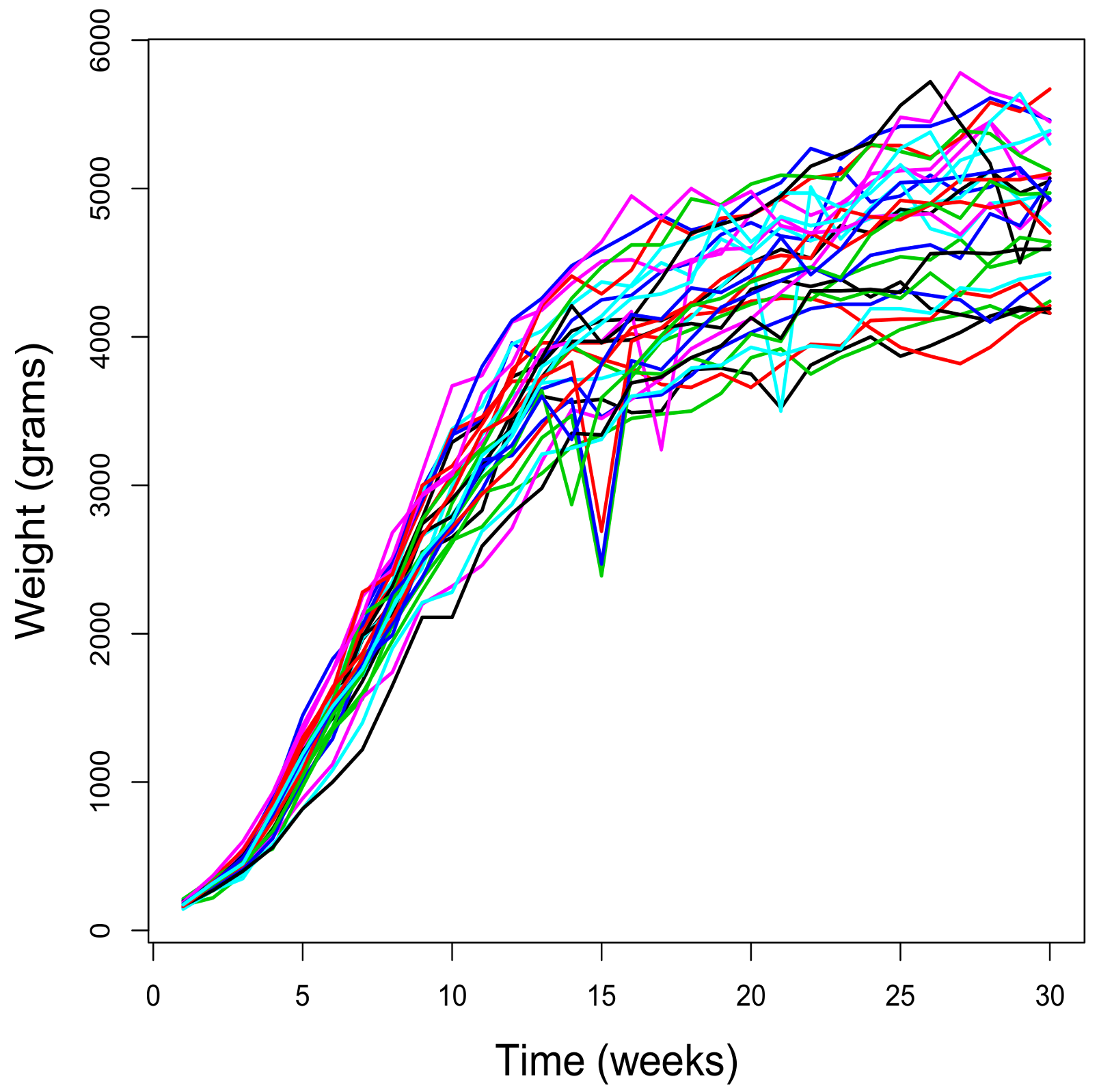
The following example is based on a study developed in [27] on some aspects related to the growth of a population of rabbits. Figure 1 shows the weight (in grams) of 29 rabbits over 30 weeks. The sample paths begin at different initial values, thus showing a sigmoidal behavior, and their bounds are dependent on the initial values. These two aspects suggest that using the Gompertz-type model proposed above would be appropriate.

This data set has been used in various papers to illustrate some aspects of the Gompertz-type process, such as the estimation of the parameters and the study of some time variables that may be of interest in the analysis of growth phenomena of this nature. As regards the estimation of the parameters, in [17] the authors designed an iterative method for solving the likelihood system of equations, while in [24] the maximization of the likelihood function was directly addressed by simulated annealing. In addition, in [28] two time variables of interest for this type of data were analyzed: concretely the inflection time and the time instant in which the process reaches a certain percentage of total growth. Both cases were modeled as first-passage time problems.

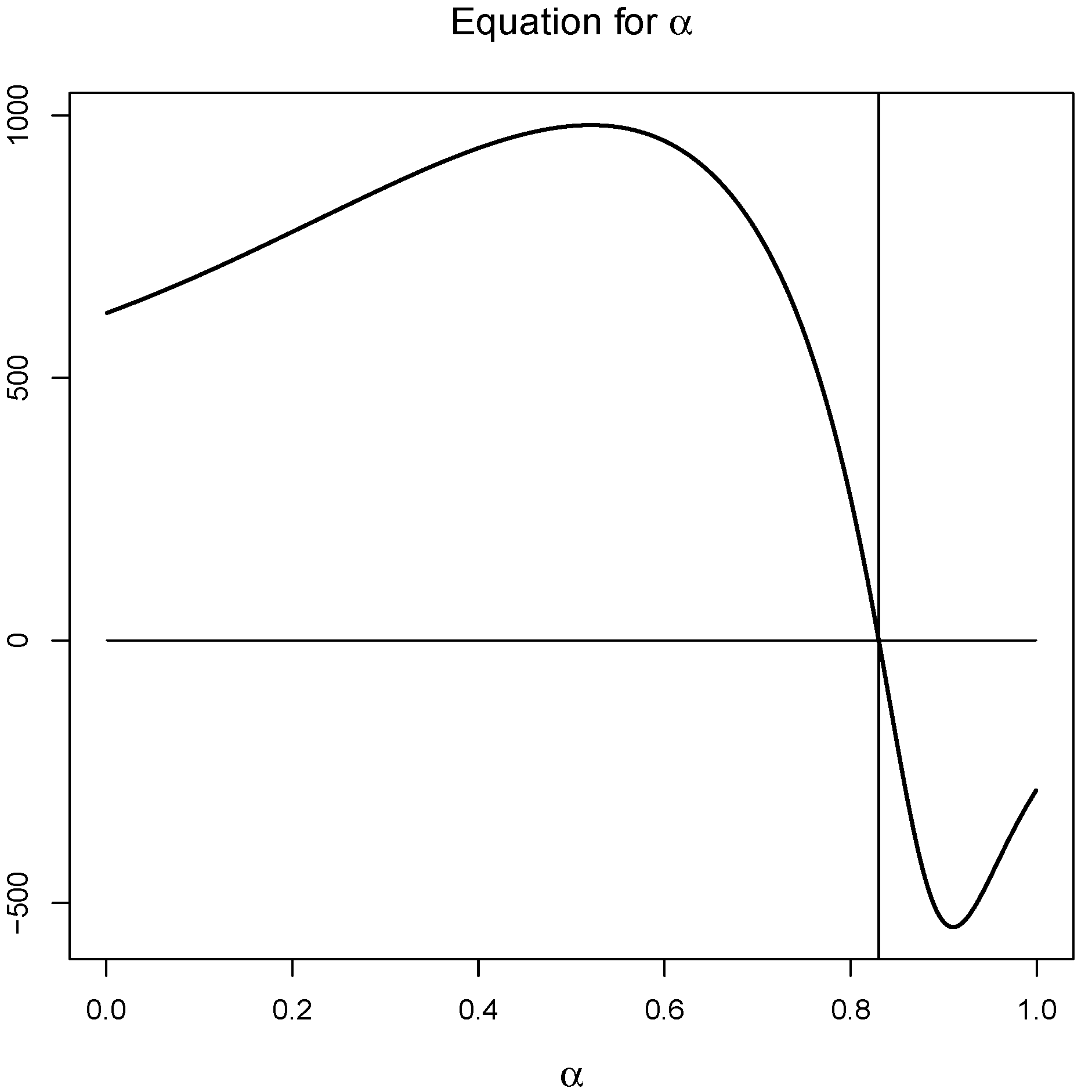
In this paper the estimation of the parameters has been carried out from the resolution of Equation (12) by means of the bisection method (see Figure 2) and then by using expressions ${\delta }^{\widehat{\alpha }}$ and ${\sigma }_{\widehat{\alpha }}^2$.

Table 2. Estimated values, standard errors and 95% confidence intervals of the parameters and the inflection time.

Parametric Function	$\mathit{\delta }$	$\mathit{\alpha }$	$\mathit{\sigma }$	g2(θ)
Estimated value	4.1020	0.8301	0.0708	7.5803
Standard error	0.0556	0.0021	0.0002	0.1053
Confidence interval	(3.9929, 4.1063)	(0.8258, 0.8343)	(0.0704, 0.0713)	(7.3738, 7.7869)

contains the estimated values for the parameters and the inflection time, as well as the asymptotic estimation error and 95% confidence intervals by applying the delta method.

As regards the weight value at the inflection time and the upper bound, remember that these values depend on the one observed at the initial instant. Taking into account the range of observed weight values at the initial instant of observation, several values have been considered within this range. For these values, the expected weight of a rabbit at the moment of inflection has been studied, as well as the possible value of the maximum weight (upper bound).

Table 3. Estimated values, standard errors, and 95% confidence intervals of the upper bound and value at the inflection time for several values of the initial weight.

Initial Weight	Upper Bound			Value at Inflection Time
	${\mathit{g}}_3(\widehat{\mathit{\theta }})$	St. Error	95% Interval	${\mathit{g}}_1(\widehat{\mathit{\theta }})$	St. Error	95% Interval
145	1772.836	70.546	(1634.568, 1911.104)	4819.068	191.764	(4443.215, 5194.920)
155	1772.836	75.411	(1625.032, 1920.640)	4819.068	204.990	(4417.295, 5220.841)
165	1883.638	80.276	(1726.298, 2040.978)	5120.260	218.215	(4692.566, 5547.954)
175	2105.243	85.142	(1938.367, 2272.118)	5722.643	231.440	(5269.028, 6176.258)
185	2216.045	90.007	(2039.634, 2392.456)	6023.835	244.665	(5544.299, 6503.371)
195	2216.045	94.872	(2030.098, 2401.992)	6023.835	257.890	(5518.378, 6529.291)
205	2105.243	99.737	(1909.760, 2300.726)	5722.643	271.115	(5191.266, 6254.020)
215	1883.638	104.603	(1678.620, 2088.657)	5120.260	284.341	(4562.961, 5677.558)

contains the estimated values, the asymptotic standard errors, and the 95% confidence intervals.

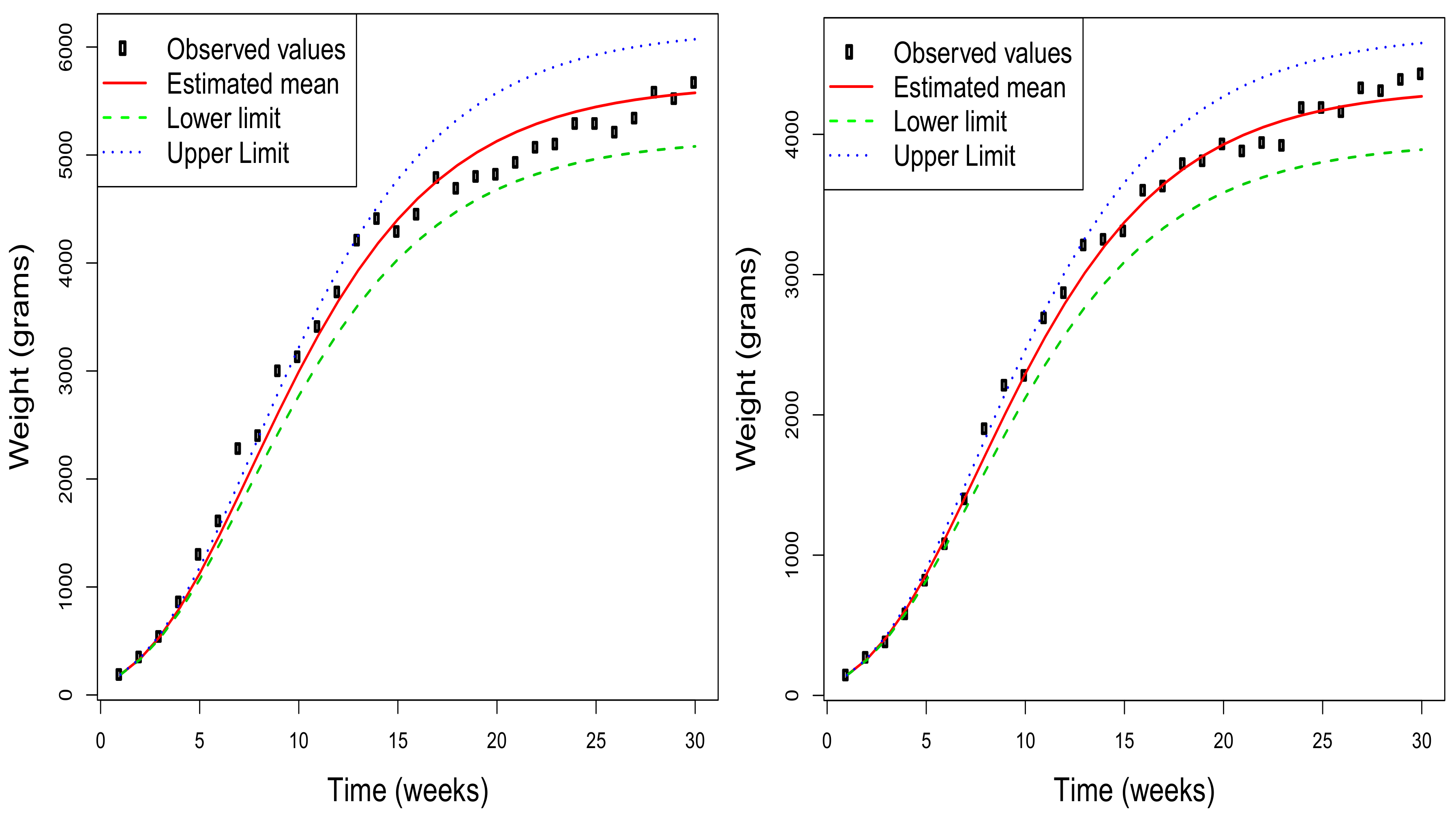
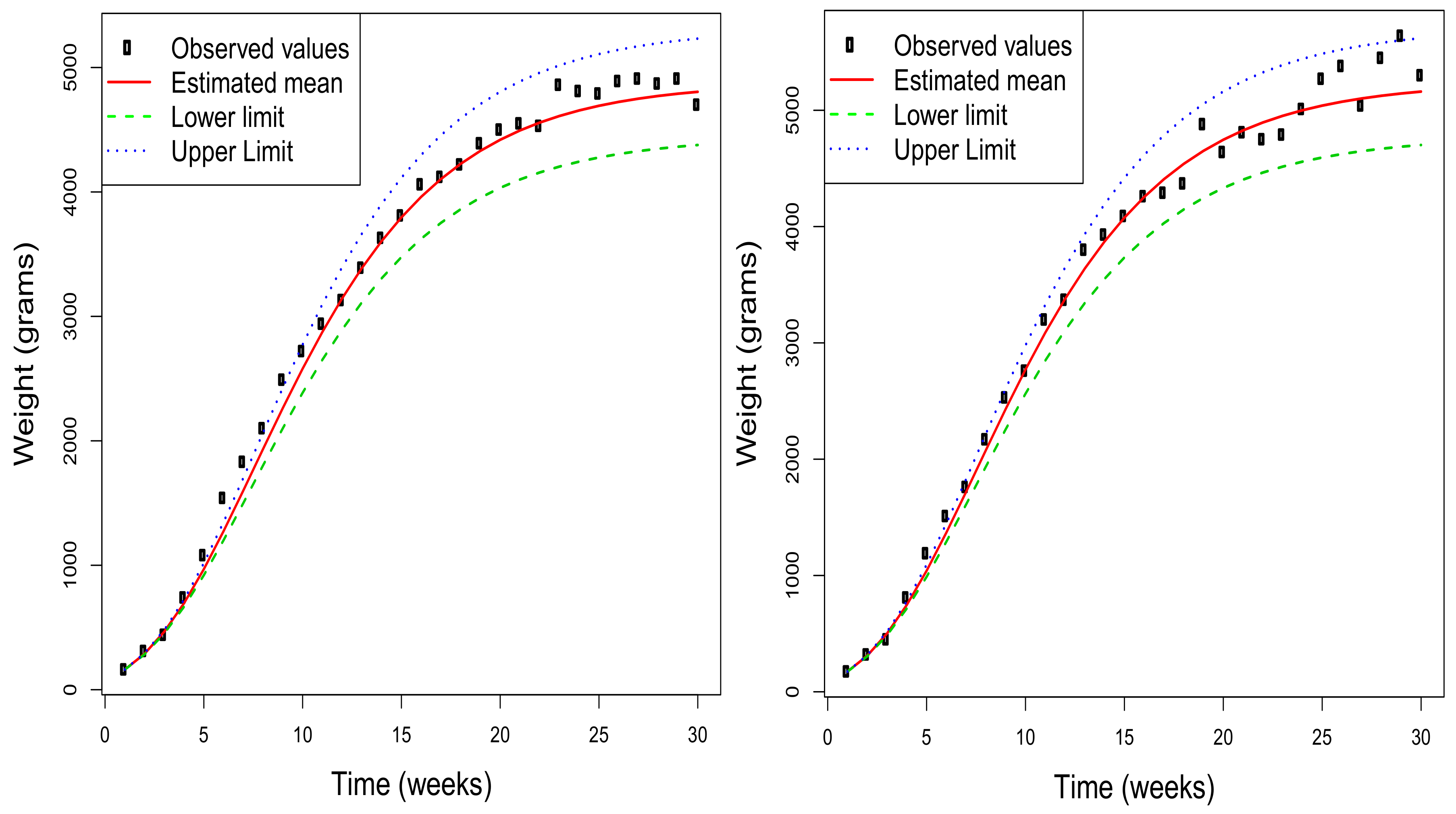
Function $E[X(t)|X(t_0)=x_0]$ can be used to provide forecasts of the weight of a rabbit that presents an initial weight $x_0$. Figure 3 shows, for a selection of four of the rabbits used in the study, the estimated mean function together with the 95% asymptotic confidence intervals obtained for each value of this function. Additionally, the observed values are included to check the quality of the adjustment made by the model under consideration. Obviously, this type of representation can also be obtained by considering any value of $x_0$ in the range of the initial distribution of the weight. Note that the estimated mean functions for each rabbit depend on the initial value, and so do the corresponding confidence intervals for the mean at each time instant. Therefore, the graphs in the figure are different for each rabbit although the estimation of the parameters is unique.

7. Conclusions

The present paper deals with some topics about inference for the non-homogeneous lognormal process (or with exogenous factors). Starting from the general form of the process, we studied the ML estimation of the parameters by using discrete sampling. This general overview enabled us to provide a unified method for several diffusion processes which can be built from particular cases of the non-homogeneous lognormal process for several choices of exogenous factors. In addition, we also looked into the asymptotic distribution of estimators, through which we can calculate the estimation errors and confidence intervals for the estimators of a wide range of parametric functions of interest in many fields. Finally, the process here described is applied to the Gompertz-type diffusion process introduced in [17].