Abstract
In this paper, we consider a stochastic diffusion process able to model the interest rate evolving with respect to time and propose a first passage time (FPT) approach through a boundary, defined as the “alert threshold”, in order to evaluate the risk of a proposed loan. Above this alert threshold, the rate is considered at the risk of usury, so new monetary policies have been adopted. Moreover, the mean FPT can be used as an indicator of the “goodness” of a loan; i.e., when an applicant is to choose between two loan offers, s/he will choose the one with a higher mean exit time from the alert boundary. An application to real data is considered by analyzing the Italian average effect global rate by means of two widely used models in finance, the Ornstein-Uhlenbeck (Vasicek) and Feller (Cox-Ingersoll-Ross) models.
1. Introduction
In recent decades, increasing attention has been paid to the study of the dynamics underlying the interest rates. The intrinsically stochastic nature of the interest rates has suggested the formulation of various models often based on stochastic differential equations (SDEs) (see, for example, [1,2] and references therein). More recently, further stochastic representations of non-usurious interest rates have been provided in order to obtain information concerning costs of loans. Most of them are simple and convenient time-homogeneous parametric models, attempting to capture certain features of observed dynamic movements, such as heteroschedasticity, long-run equilibrium, and other peculiarities (see, for example, [3,4,5]).
An interest rate is “usurious” if it is markedly above current market rates. France was the first European country to introduce an anti-usury law in 1966. In Italy, the first law of this nature (Law No. 108) was introduced in 1996. An inventory of interest rate restrictions against usury in the EU Member States was achieved at the end of 2010. In particular, the EU authorities’ attention focused on the interest rate restrictions established on precise legal rules restricting credit price, both directly by fixed thresholds as well as indirectly by intervening on the calculation of compound interest (Directorate-General of the European Commission, 2011).
Since May 2011, the Italian law has governed interest rates in loans with new regulations, fixing a threshold above which interest rates applied in loans are considered usurious. The threshold rate is based on the actual global average rate of interest (TEGM) that is quarterly determined by the Italian Ministry of Economy and Finance (Ministero dell’Economia e delle Finanze), and it is a function of various types of homogeneous transactions. Specifically, the threshold rate is calculated as 125% of the reference TEGM plus 4%. Therefore,
Moreover, the difference between the TEGM and the usury threshold cannot exceed 8%, so the maximum value admissible for TEGM cannot exceed .
Note that the penal code (art. 644, comma 4, c.p.) establishes that the scheduling of the usury interest rate takes into account errands, wages, and costs, but not taxes related to the loan supply, but, to compute the TEGM, the Bank of Italy does not consider these items. Therefore, this difference between the principle stated by the legislature and the instructions of the Bank of Italy decreases both the average rates and the threshold rates. Therefore, another boundary that is lower than that established by the Bank of Italy should be introduced. This case has also been extended to other European countries.
The basic idea of the present work is to investigate the (random) time in which an interest rate reaches an “alert boundary”, that is near the admitted limit of 0.16. To do this, we start with two classical models in the literature: Vasicek and Cox-Ingersoll-Ross (CIR) ([6,7]) since they provide good characterization of the short-term real rate process. In particular, the CIR model is able to capture the dependence of volatility on the level of interest rates ([8]).
We then investigated the first passage time (FPT) through a boundary generally depending on time. This approach is useful in economy since it suggests the time in which the trend of a loan interest rate can be considered at risk of usury, so it has to be modified from the owner of the loan service. Moreover, the mean first exit time through the alert boundary could be adopted as an indicator of the “goodness” of the loan, in the sense that an applicant choosing between two loan offers will choose the one with a higher mean exit time from the alert boundary. For the FPT analysis, we consider a constant boundary; clearly this kind of approach is applicable to other underlying models that are different from the Vasicek and CIR models and to boundaries generally depending on time, which is the case of time-dependent loan interest rate.
The layout of the paper is as follows. In Section 2, a brief review of diffusion models describing the dynamics of the interest rate is discussed. The FPT problem through a time-dependent threshold is analyzed. In Section 3, we consider data of the TEGM published by Bank of Italy. In particular, we compare the Vasicek and CIR models in order to establish which model better fits our data. Moreover, a Chow test shows the presence of structural breaks. In Section 4, the FPT problem through a constant “alert boundary” is analyzed. Concluding remarks follow.
2. Mathematical Background
We denote by the stochastic process describing the dynamics of a loan interest rate. We assume that is a time-homogeneous diffusion process defined in by the following SDE:
where and denote the drift and the infinitesimal variance of and is a standard Wiener process. The instantaneous drift represents a force that keeps pulling the process towards its long-term mean, whereas represents the amplitude of the random fluctuations. Let
be the scale function and speed density of , respectively. The transition probability density function (pdf) of , denoted by , is a solution of the Kolmogorov equation,
and of the Fokker–Planck equation,
with the delta initial conditions:
The above conditions assure the uniqueness of the transition pdf only when the endpoints of the diffusion interval are natural; otherwise, suitable boundary conditions may have to be imposed (cf., for istance, [9]).
Further, if admits a steady-state behavior, then the steady-state pdf is
Let
be the FPT variable of through a time-dependent boundary starting from , and let be its pdf. In the following, we assume that since in our context represents the initial observed value of the interest rate. The FPT problem has far-reaching implications (see, for instance, [10,11]).
As shown in [12,13], if is in , g can be obtained as a solution of the following second-kind Volterra integral equation:
where
If and are known, i.e., if the process is fixed, some closed form solution of (3) can be obtained for particular choices of the boundary . Further results have been obtained in [14,15,16]. Alternatively, a numerical algorithm can be successfully used; for example, the R package fptdApprox is also a useful instrument for the numerical evaluation of the FPT pdf (see [17,18]).
Further, if the FPT is a sure event and if is time-independent, the moments of the FPT can be evaluated via a recursive Siegert-type formula (see, for instance, [9]):
where and and given in Equation (2).
3. Modeling the Italian Loans
In this section, we consider two stochastic processes widely used in the financial literature, the Vasicek and CIR models (see [1,19]), for describing a historical series of Italian average rates on loans. We use the Akaike information criterion (AIC) as an indicator of the goodness of fit of the two models. Moreover, the presence of structural breaks is verified by means of a Chow test applied to the Euler discretization of the corresponding SDE. More precisely, the Chow test is sequentially applied for each instant in order to evaluate whether the coefficients of the Euler discretization made on each subinterval are equal to those including all observed time intervals.
TEGM values are quarterly settled and published by the Bank of Italy (see https://www.bancaditalia.it) for different types of credit transactions. We refer to the TEGM values for a particular credit transaction, “one-fifth of salary transfer”, in the period from 1 July 1997 to 31 March 2015 (data are quarterly observed, so the number of observations is 72). Moreover, two amount classes are analyzed:
- Dataset A: up to 10 million lira (until 31 December 2001) and up to € 5000 (after 2002);
- Dataset B: above 10 million lire (until 31 December 2001) and above € 5000 (after 2002).
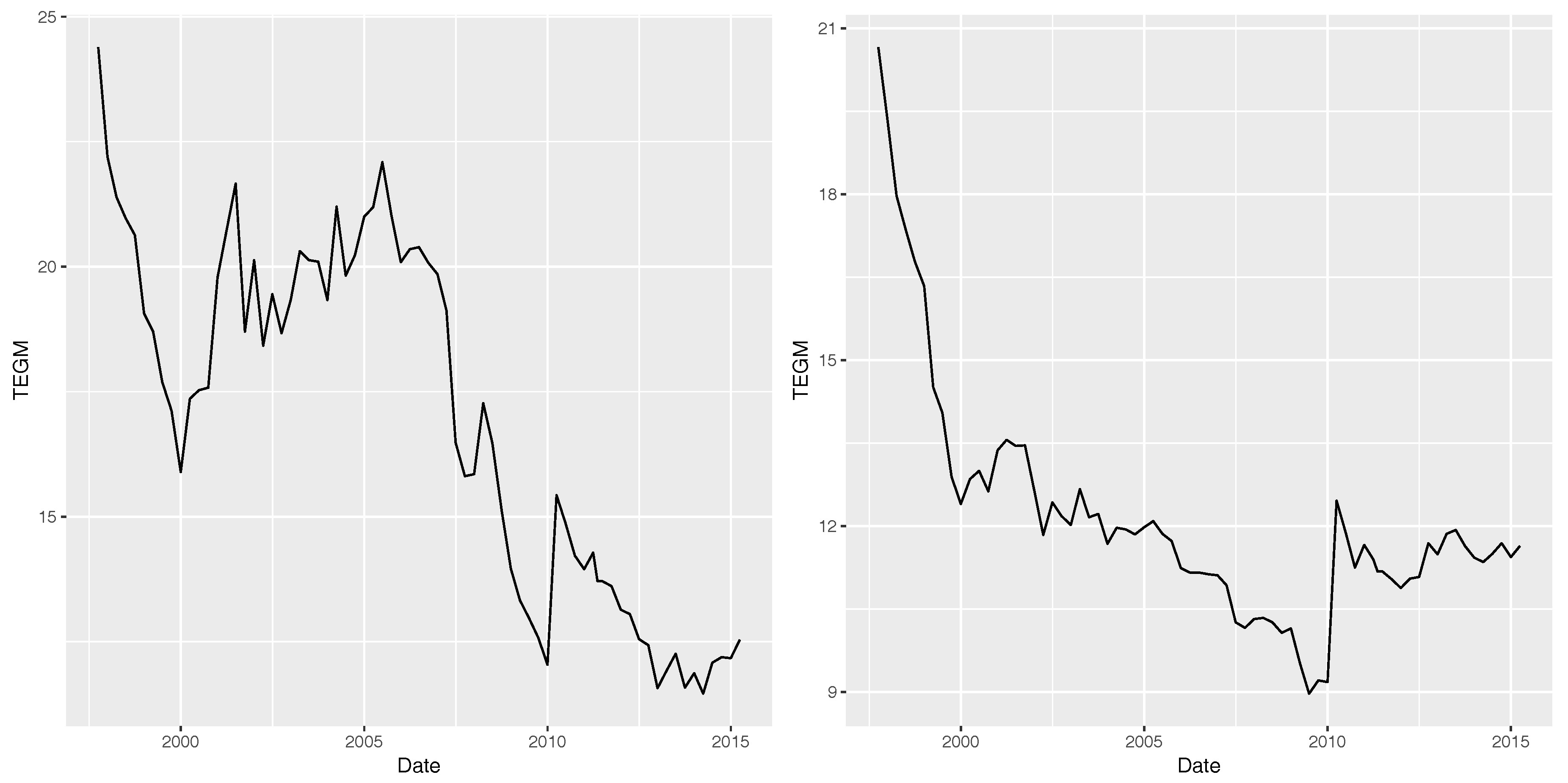
In Figure 1, Dataset A is shown on the left and Dataset B is on the right.

Figure 1.
TEGM for one-fifth of salary transfer up to € 5000 (on the left) and above € 5000 (on the right).
We estimate the parameters for the Vasiceck and CIR models, maximizing the conditional likelihood function. Specifically, we assume that the process is observed at n discrete time instants with and denote by the corresponding observations.
Let be the vector of the unknown parameters and let us assume . The likelihood function is
3.1. The Vasiceck Model
The Vasiceck model describes the short rate’s dynamics. It can be used in the evaluation of interest rate derivatives and is more suitable for credit markets. It is specified by the following SDE:
where are positive constants. The model (5) with was originally proposed by Ornstein and Uhlenbeck in 1930 in the physical context to describe the velocity of a particle moving in a fluid under the influence of friction and it was then generalized by Vasicek in 1977 to model loan interest rates. It is also used as a model and in physical and biological contexts (see, for instance, [20,21,22,23]).
We note that, for , the process is mean reverting oscillating around the equilibrium point . The process is defined in and the boundaries are natural. The transition pdf of is given by
where
represent the mean and the variance of with the condition that , respectively.
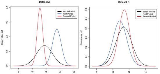
Further, has the following steady-state density:
which describes a Gaussian distribution with mean and variance .
Let be the vector of the unknown parameters. The maximum likelihood estimate is obtained as . Implementing this method, making use of the R package sde (see [24,25]), the procedure produces the results shown in Table 1. In the last row of this table, the AIC, i.e.,
is shown for the two datasets.

Table 1.
ML estimates of Model (5) for Dataset A (on the left) and for Dataset B (on the right). The last row shows the AIC.
For Datasets A and B, the Chow test applied to the Euler discretization of Model (5) shows a structural break at time , corresponding to 1 January 2008 (p-value = 0.002726) for Dataset A and at time corresponding to 1 January 2009 (p-value = 0.006231) for Dataset B. In Table 2, the ML estimates for Datasets A and B are shown considering separately the series before and after these dates. Precisely, we consider for Dataset A the following sub-periods:
Table 2.
ML estimates of Model (5) and the corresponding AIC for the periods indicated by Chow test for Dataset A (on the top) and for Dataset B (on the bottom).
- first period: 1 July 1997–1 October 2007;
- second period: 1 January 2008–31 March 2015;
for Dataset B, the sub-intervals are as follows:
- first period: 1 July 1997–1 October 2008;
- second period: 1 January 2009–31 March 2015.
The existence of a structural break is quite clear just looking at the data in Figure 1, but the Chow test permits us to establish the time at which the break verifies, and the AIC values confirm that the estimations evaluated in the two periods work better then the estimates on the whole dataset.
3.2. The CIR Model
The CIR model, originally introduced by Feller as a model for population growth in 1951, was proposed by John C. Cox, Jonathan E. Ingersoll, and Stephen A. Ross as an extension of the valuation of interest rate derivatives. It describes the evolution of interest rates, and it is characterized by the following SDE:
We point out that Model (7) has widely been used in the literature in the context of neuronal modeling (see, for example, [26,27,28]).
The process in (7) is defined in . The nature of the boundaries 0 and depends on the parameters of the process and establishes the conditions associated with the Kolmogorov and Fokker–Planck equations to determine the transition pdf. In particular, the lower boundary 0 is exit if , regular if , and entrance if , whereas the endpoint is natural (see [29]). In the following, we assume that are positive constants and that . This last condition assures that is strictly positive so that the zero state is unattainable. In this case, the 0 state is an entrance boundary, so that the transition pdf can be obtained solving the Kolmogorov and Fokker–Planck equations with the initial delta condition and a reflecting condition on the zero state. Specifically, denoting
the inverse of the scale function defined in (2), the reflecting condition for the Kolmogorov equation is
whereas, for the Fokker–Planck equation, it is
Therefore, for , one obtains
where denotes the modified Bessel function of the first kind:
and is the Euler Gamma function:
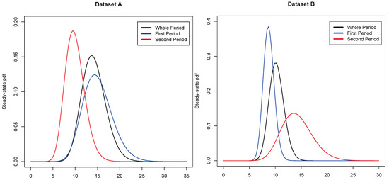
The steady-state pdf for is a Gamma distribution with shape parameter and scale parameter , i.e.,
For Model (7), in Table 3, the maximum likelihood estimates of the parameters and the standard errors and the AIC values are shown for Datasets A and B. Moreover, in the last row of this table, the AIC is shown for the two datasets.
Table 3.
ML estimates of Model (7) for Dataset A (on the left) and for Dataset B (on the right). Last row shows the AIC.
Note that the Chow test applied to the Euler discretization of Model (7) produces the same results that the Vasiceck model does. Indeed, Models (5) and (7) show the same trend, but in the CIR model one assumes residuals heteroschedasticity that does not bias the parameter estimates; it only makes the standard errors incorrect. Moreover, in Table 4, the estimates of the parameters, the standard errors, and the AIC values are shown before and after the structural breaks indicated by the Chow test. In addition, in this case, the estimates for the two separated periods work better than the estimates using only one model for the whole period shown from the AIC values.
Table 4.
ML estimates of Model (7) and the corresponding AIC for the periods indicated by the Chow test for Dataset A (on the top) and for Dataset B (on the bottom).
4. FPT Analysis for TEGM
In this section, we consider the FPT analysis for the Vasicek model. This choice is motivated by the results of Section 3. Indeed, comparing the two models by looking at the AIC values, we can see that the Vasicek model better fits our datasets in all cases (only for Dataset A does the CIR model work better than the Vasicek model).
For Datasets A and B, due to the Markovianity of the process, we consider the estimates relative to the second periods (1 January 2008–31 March 2015 for Dataset A and 1 January 2009–31 March 2015 for Dataset B) shown in Table 2.
By using the recursive Equation (4), we obtain the estimates of FPT moments for Dataset A on the period 1 January 2008–31 March 2015. In Table 5, these estimates are shown for various values of S (on the top), with corresponding to the mean of the data in the considered period, and various values of the initial point (on the bottom) fixing the alert boundary .
Table 5.
For Dataset A, second period, mean, second order moment, and variance of the random variable through various values of the threshold S (on the top) and for various values of (on the bottom).
Table 6.
For Dataset B, second period, mean, second order moment, and variance of the random variable through the threshold S for various values of S and of .
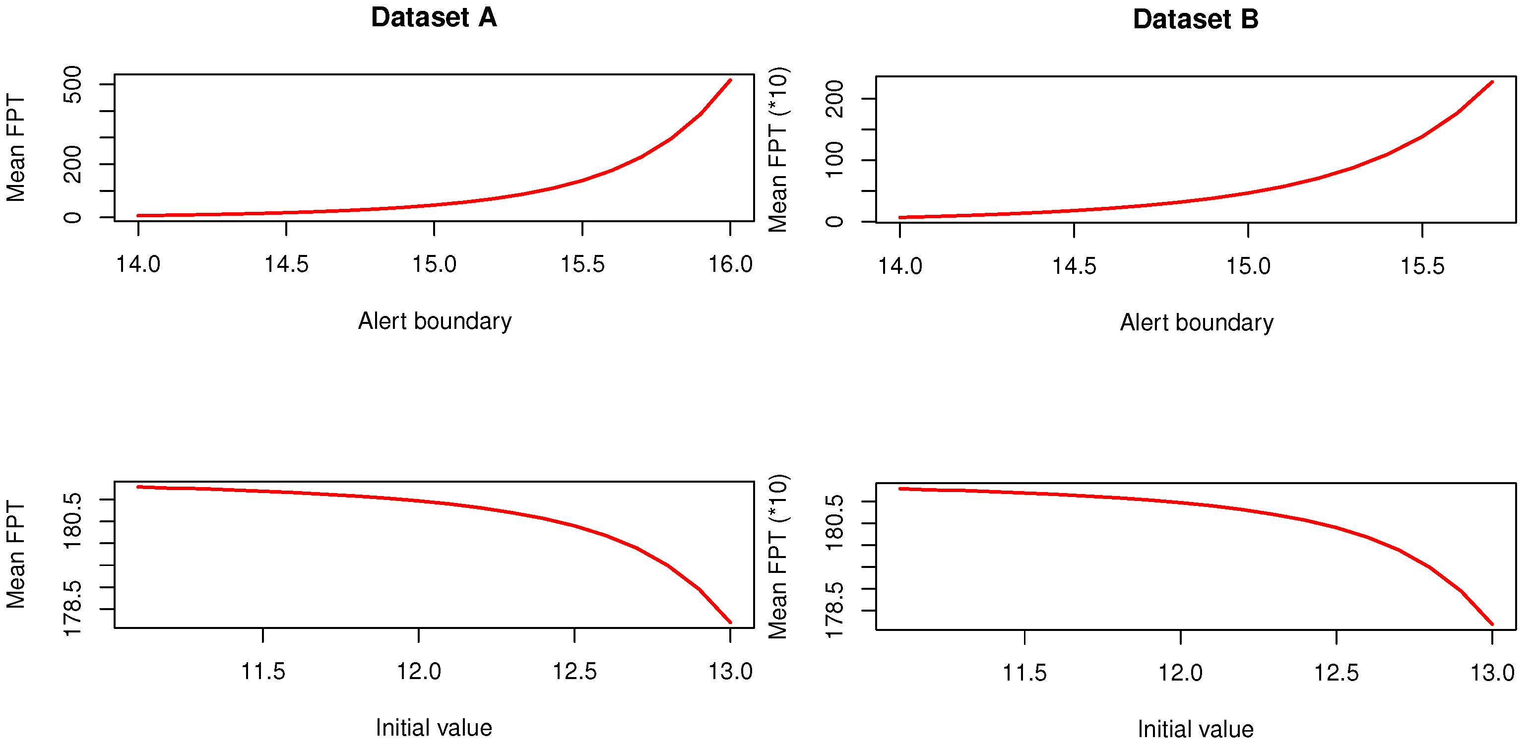
We note that, by increasing the distance between S and , the mean FPT increases. From an economic point of view, the choice of such a distance can be interpreted as a choice of “propensity of risk” of an available loan. Figure 4 shows the mean FPT (quarters starting from the loan deposit) as a function of the alert boundary (up) and as a function of the initial point . Clearly, each applicant knows the initial point and can choose the “alert boundary” S.
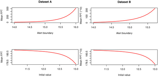
Figure 4.
Mean FPT versus the alert boundary () and the initial value () for Dataset A, second period (left), and for Dataset B, second period (right).
5. Conclusions
This paper addresses stochastic modeling of loan interest rate dynamics according to the current laws against usury. Such modeling states an upper bound, above which an interest rate is considered a usury rate and illegal. Here we focus on the Italian case and consider two models commonly used in short-term loan rates, i.e., the Vasicek and CIR models. We propose a strategy based on FPT through an alert boundary, above which the rate is considered at the risk of usury and hence has to be kept under control. Moreover, the mean first exit time through the alert boundary can be an indicator of the “goodness” of the loan, in the sense that an applicant, when he/she is choosing between two loan offers, should choose the one with a higher mean exit time from the alert boundary.
The procedure was applied to a historical series of Italian average rates on loans in the period from 1 July 1997 to 31 March 2015. We considered “one-fifth of salary transfer” and two amount classes were analyzed: (a) up to 10 million lira (until 31 December 2001) and up to € 5000 (after 2002); and (b) above 10 million lire (until 31 December 2001) and above € 5000 (after 2002). The model parameters were estimated by MLE, and a Chow test was applied to detect the presence of structural breaks in our datasets.
The model and proposed strategy are apt for further development. Indeed, we can extend the analysis to more general processes in which some parameters are time-dependent, or we can consider time-dependent thresholds to model varying loan interest rates. Further generalization can include analysis of FPT through two boundaries: the upper one describing an alert threshold and the lower one representing a favorable interest rate.
Author Contributions
Giuseppina Albano and Virginia Giorno contributed equally in the writing of this work.
Acknowledgments
This paper was supported partially by INDAM-GNCS.
Conflicts of Interest
The authors declare no conflict of interest.
References
- Brigo, B.; Mercurio, F. Interest Rate Models-Theory and Practice with Smile, Inflation and Credit; Springer: Berlin, Germany, 2007. [Google Scholar]
- Buetow, G.W., Jr.; Hanke, B.; Fabozzi, F.J. Impact of different interest rate models on bound value measures. J. Fixed Income 2001, 3, 41–53. [Google Scholar] [CrossRef]
- Fan, J.; Jiang, J.; Zhang, C.; Zhou, Z. Time-dependent diffusion models for term structure dynamics. Stat. Sin. 2003, 13, 965–992. [Google Scholar]
- Chen, W.; Xu, L.; Zhu, S.P. Stock loan valuation under a stochastic interest rate model. Comput. Math. Appl. 2015, 70, 1757–1771. [Google Scholar] [CrossRef]
- Di Lorenzo, E.; Orlando, A.; Sibillo, M. A Stochastic model fro loan interest rates. Banks Bank Syst. 2013, 8, 94–99. [Google Scholar]
- Cox, J.C.; Ingersoll, J.E.; Ross, S.A. A Theory of the Term Structure of Interest Rates. Econometrica 1985, 53, 385–407. [Google Scholar] [CrossRef]
- Vasicek, O. An equilibrium characterization of the term structure. J. Financ. Econ. 1977, 5, 177–188. [Google Scholar] [CrossRef]
- Khramov, V. Estimating Parameters of Short-Term Real Interest Rate Models; IMF Working Papers; International Monetary Fund: Washington, DC, USA, 2012. [Google Scholar]
- Ricciardi, L.M.; Di Crescenzo, A.; Giorno, V.; Nobile, A.G. An outline of theoretical and algorithmic approaches to first passage time problems with applications to biological modeling. Math. Jpn. 1999, 50, 247–322. [Google Scholar]
- Albano, G.; Giorno, V.; Román-Román, P.; Torres-Ruiz, F. On the effect of a therapy able to modify both the growth rates in a Gompertz stochastic model. Math. Biosci. 2013, 245, 12–21. [Google Scholar] [CrossRef] [PubMed]
- Albano, G.; Giorno, V.; Román-Román, P.; Torres-Ruiz, F. On a Non-homogeneous Gompertz-Type Diffusion Process: Inference and First Passage Time. In Computer Aided Systems Theory-EUROCAST; Moreno Diaz, R., Pichler, F., Quesada Arencibia, A., Eds.; Lecture Notes in Computer Science; Springer: Cham, Switzerland, 2017; Volume 10672, pp. 47–54. [Google Scholar]
- Buonocore, A.; Nobile, A.G.; Ricciardi, L.M. A new integral equation for the evaluation of first-passage-time probability densitie. Adv. Appl. Prob. 1987, 19, 784–800. [Google Scholar] [CrossRef]
- Giorno, V.; Nobile, A.G.; Ricciardi, L.M.; Sato, S. On the evaluation of firtst-passage-time probability densities via non-singular integral equations. Adv. Appl. Prob. 1989, 21, 20–36. [Google Scholar] [CrossRef]
- Buonocore, A.; Caputo, L.; D’Onofrio, G.; Pirozzi, E. Closed-form solutions for the first-passage-time problem and neuronal modeling. Ricerche di Matematica 2015, 64, 421–439. [Google Scholar] [CrossRef]
- Di Crescenzo, A.; Giorno, V.; Nobile, A.G. Analysis of reflected diffusions via an exponential time-based transformation. J. Stat. Phys. 2016, 163, 1425–1453. [Google Scholar] [CrossRef]
- Abundo, M. The mean of the running maximum of an integrated Gauss–Markov process and the connection with its first-passage time. Stoch. Anal. Appl. 2017, 35, 499–510. [Google Scholar] [CrossRef]
- Román-Román, P.; Serrano-Pérez, J.; Torres-Ruiz, F. More general problems on first-passage times for diffusion processes: A new version of the fptdapprox r package. Appl. Math. Comput. 2014, 244, 432–446. [Google Scholar] [CrossRef]
- Román-Román, P.; Serrano-Pérez, J.; Torres-Ruiz, F. fptdapprox: Approximation of First-Passage-Time Densities for Diffusion Processes, R Package Version 2.1, 2015. Available online: http://cran.r-project.org/package=fptdApprox (accessed on 23 November 2017).
- Linetsky, V. Computing hitting time densities for CIR and OU diffusions: Applications to mean reverting models. J. Comput. Financ. 2004, 4, 1–22. [Google Scholar] [CrossRef]
- Albano, G.; Giorno, V. A stochastic model in tumor growth. J. Theor. Biol. 2006, 242, 229–236. [Google Scholar] [CrossRef] [PubMed]
- Buonocore, A.; Caputo, L.; Nobile, A.G.; Pirozzi, E. Restricted Ornstein–Uhlenbeck process and applications in neuronal models with periodic input signals. J. Comp. Appl. Math. 2015, 285, 59–71. [Google Scholar] [CrossRef]
- Dharmaraja, S.; Di Crescenzo, A.; Giorno, V.; Nobile, A.G. A continuous-time Ehrenfest model with catastrophes and its jump-diffusion approximation. J. Stat. Phys. 2015, 161, 326–345. [Google Scholar] [CrossRef]
- Giorno, V.; Spina, S. On the return process with refractoriness for non-homogeneous Ornstein–Uhlenbeck neuronal model. Math. Biosci. Eng. 2014, 11, 285–302. [Google Scholar] [PubMed]
- Iacus, S.M. Simulation and Inference for Stochastic Differential Equations with R Examples; Springer Series in Statistics: Berlin, Germany, 2008. [Google Scholar]
- Iacus, S.M. sde-Manual and Help on Using the sde R Package. 2009. Available online: http://www.rdocumentation.org/packages/sde/versions/2.0.9 (accessed on 24 October 2017).
- Giorno, V.; Lanský, P.; Nobile, A.G.; Ricciardi, L.M. Diffusion approximation and first-passage-time problem for a model neuron. III. A birth-and-death process approach. Biol. Cybern. 1988, 58, 387–404. [Google Scholar] [CrossRef] [PubMed]
- Giorno, V.; Nobile, A.G.; Ricciardi, L.M. Single neuron’s activity: On certain problems of modeling and interpretation. BioSystems 1997, 40, 65–74. [Google Scholar] [CrossRef]
- Nobile, A.G.; Pirozzi, E. On time non-homogeneous Feller-type diffusion process in neuronal modeling. In Computer Aided Systems Theory-EUROCAST 2017; Moreno Diaz, R., Pichler, F., Quesada Arencibia, A., Eds.; Lecture Notes in Computer Science; Springer: Cham, Switzerland, 2015; Volume 9520, pp. 183–191. [Google Scholar]
- Karlin, S.; Taylor, H.W. A Second Course in Stochastic Processes; Academic Press: New York, NY, USA, 1981. [Google Scholar]

© 2018 by the authors. Licensee MDPI, Basel, Switzerland. This article is an open access article distributed under the terms and conditions of the Creative Commons Attribution (CC BY) license (http://creativecommons.org/licenses/by/4.0/).