On the Bounds for a Two-Dimensional Birth-Death Process with Catastrophes

Abstract

The model of a two-dimensional birth-death process with possible catastrophes is studied. The upper bounds on the rate of convergence in some weighted norms and the corresponding perturbation bounds are obtained. In addition, we consider the detailed description of two examples with 1-periodic intensities and various types of death (service) rates. The bounds on the rate of convergence and the behavior of the corresponding mathematical expectations are obtained for each example.

1. Introduction

There is a large number of papers devoted to the research of continuous-time Markov chains and models with possible catastrophes, see for instance [1,2,3,4,5,6,7,8,9,10,11,12,13,14,15,16,17,18,19,20,21], and the references therein. Such models are widely used in queueing theory and biology, particularly, for simulations in hight-performance computing. In some recent papers, the authors deal with more or less special birth-death processes with additional transitions from and to origin [9,10,11,12,13,18,19,20]. In [22], a general class of Markovian queueing models with possible catastrophes is analyzed and some bounds on the rate of convergence are obtained. Here we consider a more specific but important model of a two-dimensional birth-death process with possible catastrophes and obtain the upper bounds on the rate of convergence in some weighted norms and the corresponding perturbation bounds.

Ergodicity bounds in l-1 norm (associated with total variation) for such processes can be obtained quite easily due to the possibility of catastrophes, i.e., transitions to zero from any other state. Obtaining the estimates in weighted norms that guarantee the convergence of the corresponding mathematical expectations as well as the construction of the corresponding limiting characteristics are more complex problems.

In addition, we consider in detail two examples with 1-periodic intensities and various types of death (service) rates. The bounds on the rate of convergence and the behavior of the corresponding mathematical expectations are obtained for each example.

Our results seem to be interesting for both queueing theory and biology applications.

Let $\mathbf{X}(t)=(X_1(t),X_2(t))$ be two-dimensional birth-death-catastrophe process (where $X_i(t)$ is the corresponding number of particles of type i, $i=1,2$) such that in the interval $(t,t+h)$ the following transitions are possible with order h: birth of a particle of type i, death of a particle of type i, and catastrophe (or transition to the zero state $\mathbf{0}=(0,0)$).

Denote by ${\lambda }_{1,i,j}(t)$, ${\lambda }_{2,i,j}(t)$, ${\mu }_{1,i,j}(t)$, ${\mu }_{2,i,j}(t)$, and by ${\xi }_{i,j}(t)$ corresponding birth, death, and catastrophe rates for the process. Namely, ${\lambda }_{1,i,j}(t)$ is the rate of transition from state $(i,j)$ to state $(i+1,j)$ at the moment t, ${\lambda }_{2,i,j}(t)$ is the rate of transition from state $(i,j)$ to state $(i,j+1)$, ${\mu }_{1,i,j}(t)$ is the rate of transition from state $(i,j)$ to state $(i-1,j)$, ${\mu }_{2,i,j}(t)$ is the rate of transition from state $(i,j)$ to state $(i,j-1)$, and finally, ${\xi }_{i,j}(t)$ is the rate of transition from state $(i,j)$ to state $(0,0)$ at the moment t.

The transition rate diagram associated with the process is presented in Figure 1.

Suppose that all intensities are nonnegative and locally integrable on $[0;\infty )$ as functions of t. Moreover, we also suppose that the condition of boundedness

$${\lambda }_{1,i,j}(t)+{\lambda }_{2,i,j}(t)+{\mu }_{1,i,j}(t)+{\mu }_{2,i,j}(t)+{\xi }_{i,j}(t)\le L<\infty ,$$

(1)

hold for any $i,j$ and almost all $t\ge 0$.

We renumber the states of two-dimensional process $\mathbf{X}(t)=(X_1(t),X_2(t))$ (0,0), (0,1), (1,0), (0,2), (1,1), (2,0), … by increasing the sum of coordinates, and in the case of the same sum, by increasing the first coordinate. Hence we obtain one-dimensional vector $\mathbf{p}(t)={\left(p_0(t),p_1(t),\cdots \right)}^T$ of state probabilities in a new numeration, and therefore, we can rewrite the forward Kolmogorov system in the following form:

$$\frac{d\mathbf{p}}{dt}=\mathbf{A}\left(t\right)\mathbf{p},t\ge 0,$$

(2)

where $\mathbf{A}(t)=\left(a_{ij}(t)\right)$ is the corresponding transposed intensity matrix: $\mathbf{A}(t)=\left(\begin{array}{ccccccccccc}{a}_{00}& {\mu }_{1,0,1}+{\xi }_{0,1}& {\mu }_{2,1,0}+{\xi }_{1,0}& {\xi }_{0,2}& {\xi }_{1,1}& {\xi }_{2,0}& {\xi }_{0,3}& {\xi }_{1,2}& {\xi }_{2,1}& {\xi }_{3,0}& \cdots \\ {\lambda }_{1,0,0}& a_{11}& 0& {\mu }_{1,0,2}& {\mu }_{2,1,1}& 0& 0& 0& 0& 0& \cdots \\ {\lambda }_{2,0,0}& 0& a_{22}& 0& {\mu }_{1,1,1}& {\mu }_{2,2,0}& 0& 0& 0& 0& \cdots \\ 0& {\lambda }_{1,0,1}& 0& a_{33}& 0& 0& {\mu }_{1,0,3}& {\mu }_{2,1,2}& 0& 0& \cdots \\ 0& {\lambda }_{2,0,1}& {\lambda }_{1,1,0}& 0& a_{44}& 0& 0& {\mu }_{1,1,2}& {\mu }_{2,2,1}& 0& \cdots \\ 0& 0& {\lambda }_{2,1,0}& 0& 0& a_{55}& 0& 0& {\mu }_{1,2,1}& {\mu }_{2,3,0}& \cdots \\ 0& 0& 0& {\lambda }_{1,0,2}& 0& 0& a_{66}& 0& 0& 0& \cdots \\ \cdots & \cdots & \cdots & \cdots & \cdots & \cdots & \cdots & \cdots & \cdots \end{array}\right),$ and $a_{ii}(t)=-{\sum }_i{a}_{i,j}(t)$.

Throughout the paper by $\parallel ·\parallel$ we denote the $l_1$-norm, i. e., $\parallel \mathbf{x}\parallel =\sum |x_i|$, and $\parallel B\parallel ={sup}_j{\sum }_i|b_{ij}|$ for $B={(b_{ij})}_{i,j=0}^{\infty }$.

Let $\mathsf{\Omega }$ be a set all stochastic vectors, i.e., $l_1$ vectors are with nonnegative coordinates and unit norm. Hence the assumption (1) implies the bound $\parallel \mathbf{A}(t)\parallel \le 2L$ for almost all $t\ge 0$. Therefore, the operator function $\mathbf{A}(t)$ from $l_1$ into itself is bounded for almost all $t\ge 0$ and locally integrable on $[0;\infty )$. Therefore, we can consider the forward Kolmogorov system as a differential equation in the space $l_1$ with bounded operator.

It is well known, see [23], that the Cauchy problem for such a differential equation has a unique solution for an arbitrary initial condition, and $\mathbf{p}(s)\in \mathsf{\Omega }$ implies $\mathbf{p}(t)\in \mathsf{\Omega }$ for $t\ge s\ge 0$.

We have

$$\mathbf{p}(t)=U(t,s)\mathbf{p}(s),$$

(3)

where $U(t,s)$ is the Cauchy operator of Equation (2).

Note that the vector of state probabilities can be written in ’two-dimensional form’ as $\mathbf{p}(t)={\left(p_{00}(t),p_{01}(t),p_{10}(t),p_{02}(t),p_{11}(t),\cdots \right)}^T$.

2. Bounds in ${\mathit{l}}_{\mathbf{1}}$ Norm

Consider the first equation in forward Kolmogorov system and rewrite it in the following form:

$$\frac{d{p}_0}{dt}=-\left(a_{00}+\xi (t)\right)p_0+\sum _{i\ge 1}(a_{0i}(t)-\xi (t))p_i+\xi (t),$$

(4)

where $\xi (t)={inf}_{i,j}{\xi }_{i,j}(t)$.

Then we have from Equation (2) the following system:

$$\frac{d\mathbf{p}}{dt}=B(t)\mathbf{p}+\mathbf{f}(t),$$

(5)

where $\mathbf{f}(t)={(\xi (t),0,\dots )}^T$ and $B(t)=\left(\begin{array}{ccccccccccc}{a}_{00}-\xi & {\mu }_{1,0,1}+{\xi }_{0,1}-\xi & {\mu }_{2,1,0}+{\xi }_{1,0}-\xi & {\xi }_{0,2}-\xi & {\xi }_{1,1}-\xi & {\xi }_{2,0}-\xi & {\xi }_{0,3}-\xi & {\xi }_{1,2}-\xi & {\xi }_{2,1}-\xi & {\xi }_{3,0}-\xi & \cdots \\ {\lambda }_{1,0,0}& a_{11}& 0& {\mu }_{1,0,2}& {\mu }_{2,1,1}& 0& 0& 0& 0& 0& \cdots \\ {\lambda }_{2,0,0}& 0& a_{22}& 0& {\mu }_{1,1,1}& {\mu }_{2,2,0}& 0& 0& 0& 0& \cdots \\ 0& {\lambda }_{1,0,1}& 0& a_{33}& 0& 0& {\mu }_{1,0,3}& {\mu }_{2,1,2}& 0& 0& \cdots \\ 0& {\lambda }_{2,0,1}& {\lambda }_{1,1,0}& 0& a_{44}& 0& 0& {\mu }_{1,1,2}& {\mu }_{2,2,1}& 0& \cdots \\ 0& 0& {\lambda }_{2,1,0}& 0& 0& a_{55}& 0& 0& {\mu }_{1,2,1}& {\mu }_{2,3,0}& \cdots \\ 0& 0& 0& {\lambda }_{1,0,2}& 0& 0& a_{66}& 0& 0& 0& \cdots \\ \cdots & \cdots & \cdots & \cdots & \cdots & \cdots & \cdots & \cdots & \cdots \end{array}\right).$

We have

$$\mathbf{p}(t)=V(t)\mathbf{p}(0)+{\int }_0^{t}V(t,\tau )\mathbf{f}(\tau )d\tau ,$$

(6)

where $V(t,\tau )$ is the Cauchy operator of Equation (5).

Then one can estimate the logarithmic norm of $B(t)$ in the space of sequences $l_1$ (see [24]):

$$\begin{gathered} \gamma {\left(B(t)\right)}_1=max\left(a_{00}(t)-\xi (t)+\sum _{i\ge 1}{a}_{i0}(t),\right. \\ \left.\underset{i\ge 1}{sup}\left(a_{ii}(t)+a_{0i}(t)-\xi (t)+\sum _{j\ne i,j\ge 1}{a}_{ji}(t)\right)\right)=-\xi (t). \end{gathered}$$

(7)

Then for all $0\le s\le t$ we have

$$\parallel V(t,s)\parallel \le e^{-\underset{s}{\overset{t}{\int }}\xi (\tau )d\tau }.$$

(8)

Therefore, the following statement is correct (see details in [16,18]).

Theorem 1.

Let the intensities of catastrophes be essential, that is

$${\int }_0^{\infty }\xi (t)dt=\infty .$$

(9)

Then the process $\mathbf{X}(t)$ is weakly ergodic and the following bound of the rate of convergence holds:

$$\begin{array}{c}\hfill ∥{\mathbf{p}}^{\ast }(t)-{\mathbf{p}}^{\ast \ast }(t)∥\le 2e^{-\underset{0}{\overset{t}{\int }}\xi (\tau )d\tau },\end{array}$$

(10)

for all initial conditions ${\mathbf{p}}^{\ast }(0),{\mathbf{p}}^{\ast \ast }(0)$ and any $t\ge 0$.

Consider now the ”perturbed” process $\overline{\mathbf{X}}=\overline{\mathbf{X}}(t)$, $t\ge 0$, adding a dash on top for all corresponding characteristics.

Put $\widehat{\mathbf{A}}(t)=\mathbf{A}(t)-\overline{\mathbf{A}}(t)$, and assume that the perturbations are “uniformly small”, i.e., for almost all $t\ge 0$ the following inequality is correct

$$\parallel \widehat{\mathbf{A}}(t)\parallel \le \epsilon .$$

(11)

Consider the stability bounds of the process $\mathbf{X}(t)$ under these perturbations. In addition, we assume that the process is exponentially ergodic, that is, that for some positive $M,a$ and for all s, t, $0\le s\le t$ the following inequality holds

$$e^{-{\int }_s^t\xi (u)du}\le M{e}^{-a(t-s)}.$$

(12)

Then from Theorem 1:

$$\parallel {\mathbf{p}}^{\ast }(t)-{\mathbf{p}}^{\ast \ast }(t)\parallel \le e^{-\underset{s}{\overset{t}{\int }}\xi (\tau )d\tau }\parallel {\mathbf{p}}^{\ast }(s)-{\mathbf{p}}^{\ast \ast }(s)\parallel \le 2e^{-\underset{s}{\overset{t}{\int }}\xi (\tau )d\tau }\le 2M{e}^{-a(t-s)}.$$

(13)

Here we apply the approach proposed in [25] for a stationary case and generalized for a nonstationary situation in [15,16].

We have

$$\parallel \mathbf{p}(t)-\overline{\mathbf{p}}(t)\parallel \le M{e}^{-a(t-s)}\parallel \mathbf{p}(s)-\overline{\mathbf{p}}(s)\parallel +M{\int }_s^t\parallel \widehat{A}(u)\parallel e^{-a(u-s)}du.$$

(14)

Therefore we obtain

$$\parallel \mathbf{p}(t)-\overline{\mathbf{p}}(t)\parallel \le \left\{\begin{array}{c}\parallel \mathbf{p}(s)-\overline{\mathbf{p}}(s)\parallel +(t-s)\epsilon ,0<t<a^{-1}logM,\hfill \\ a^{-1}(logM+1-M{e}^{-a(t-s)})\epsilon +M{e}^{-a(t-s)}\parallel \mathbf{p}(s)-\overline{\mathbf{p}}(s)\parallel ,t\ge a^{-1}logM.\hfill \end{array}\right.$$

(15)

It implies the following statement.

Theorem 2.

If the condition (12) is fulfilled and the perturbations are uniformly small:

$$\parallel \widehat{A}(t)\parallel \le \epsilon ,$$

(16)

for almost all $t\ge 0$. Then the following bound holds:

$$\underset{t\to \infty }{lim\; sup}∥\mathbf{p}(t)-\overline{\mathbf{p}}(t)∥\le \frac{\epsilon \left(1+logM\right)}{a},$$

(17)

for any initial conditions $\mathbf{p}(0)$, $\overline{\mathbf{p}}(0)$.

Corollary 1.

Let the intensities of the process be 1-periodic and instead of (12) we have the following inequality

$${\int }_0^1\xi (t)dt\ge \theta >0.$$

(18)

Then (17) is correct for

$$M=e^K,a=\theta ,$$

(19)

where $K={sup}_{|t-s|\le 1}{\int }_s^t\xi (\tau )d\tau <\infty$.

3. Bounds in Weighted Norms

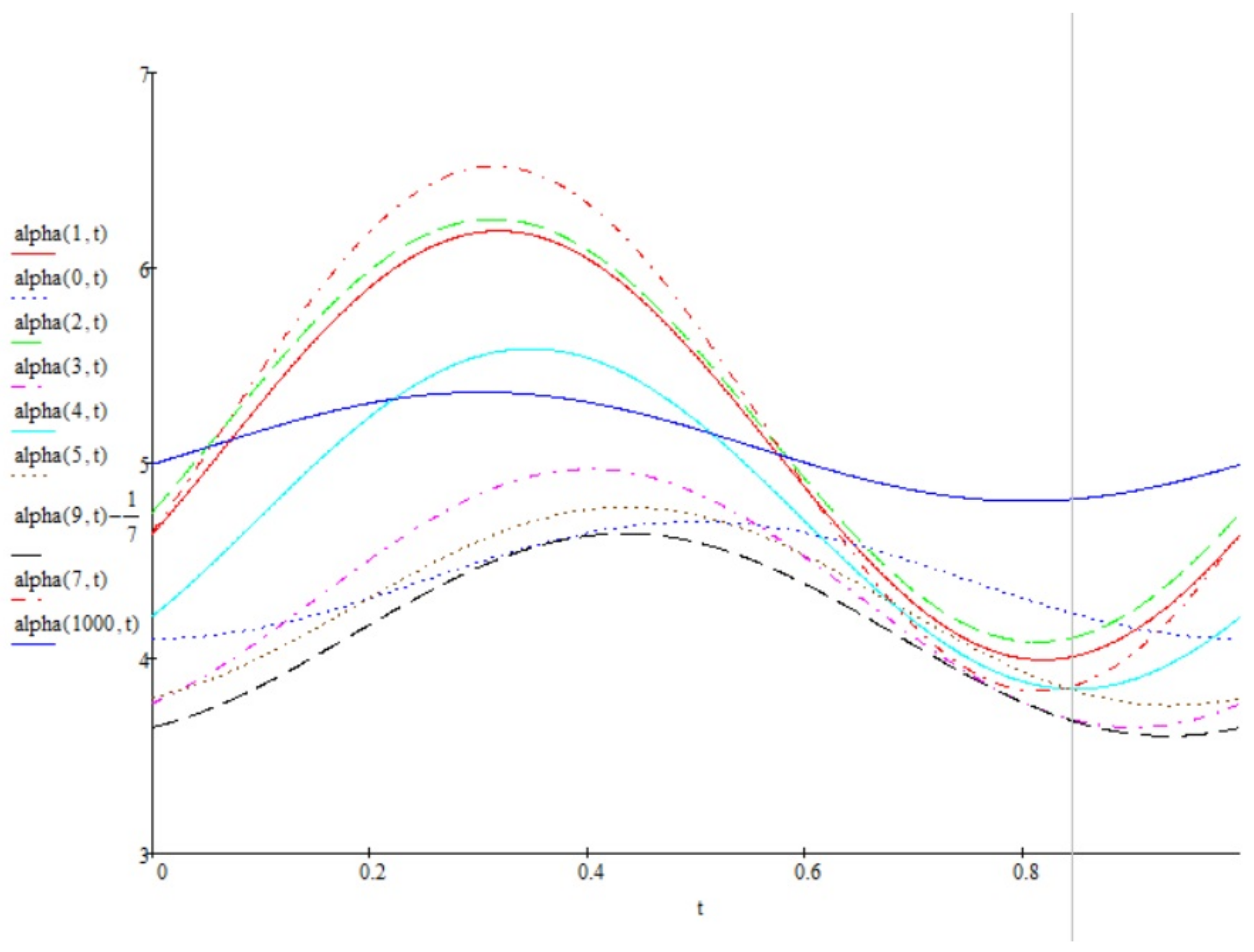
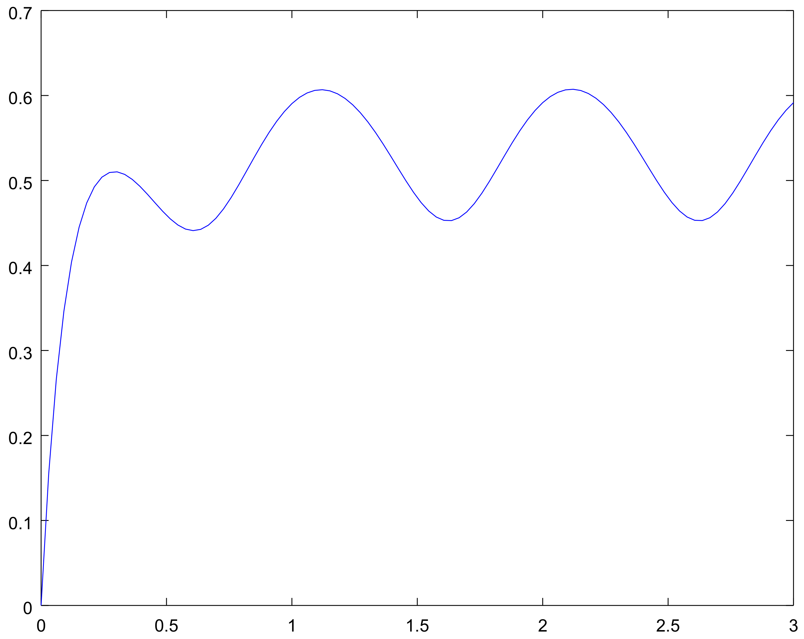
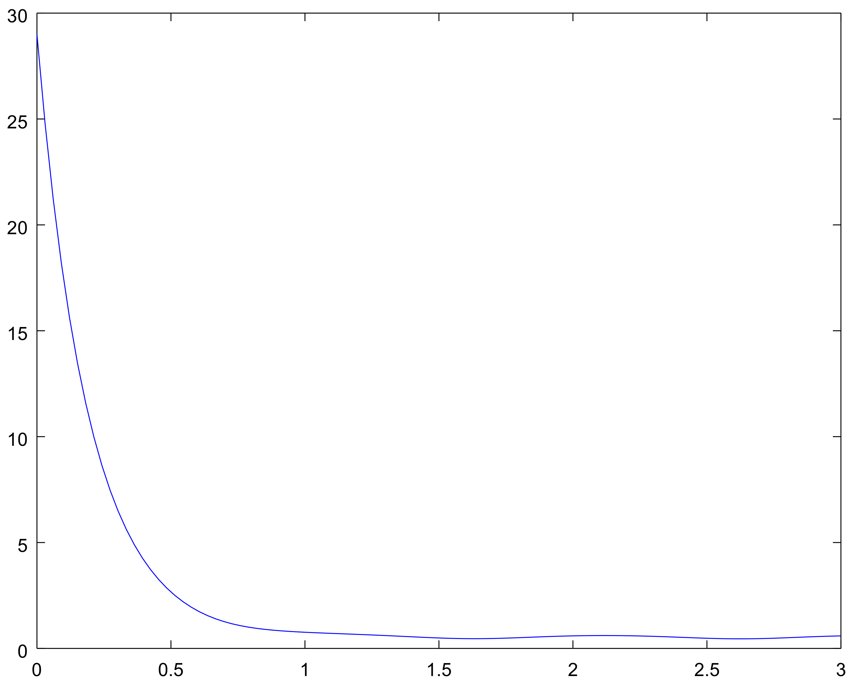
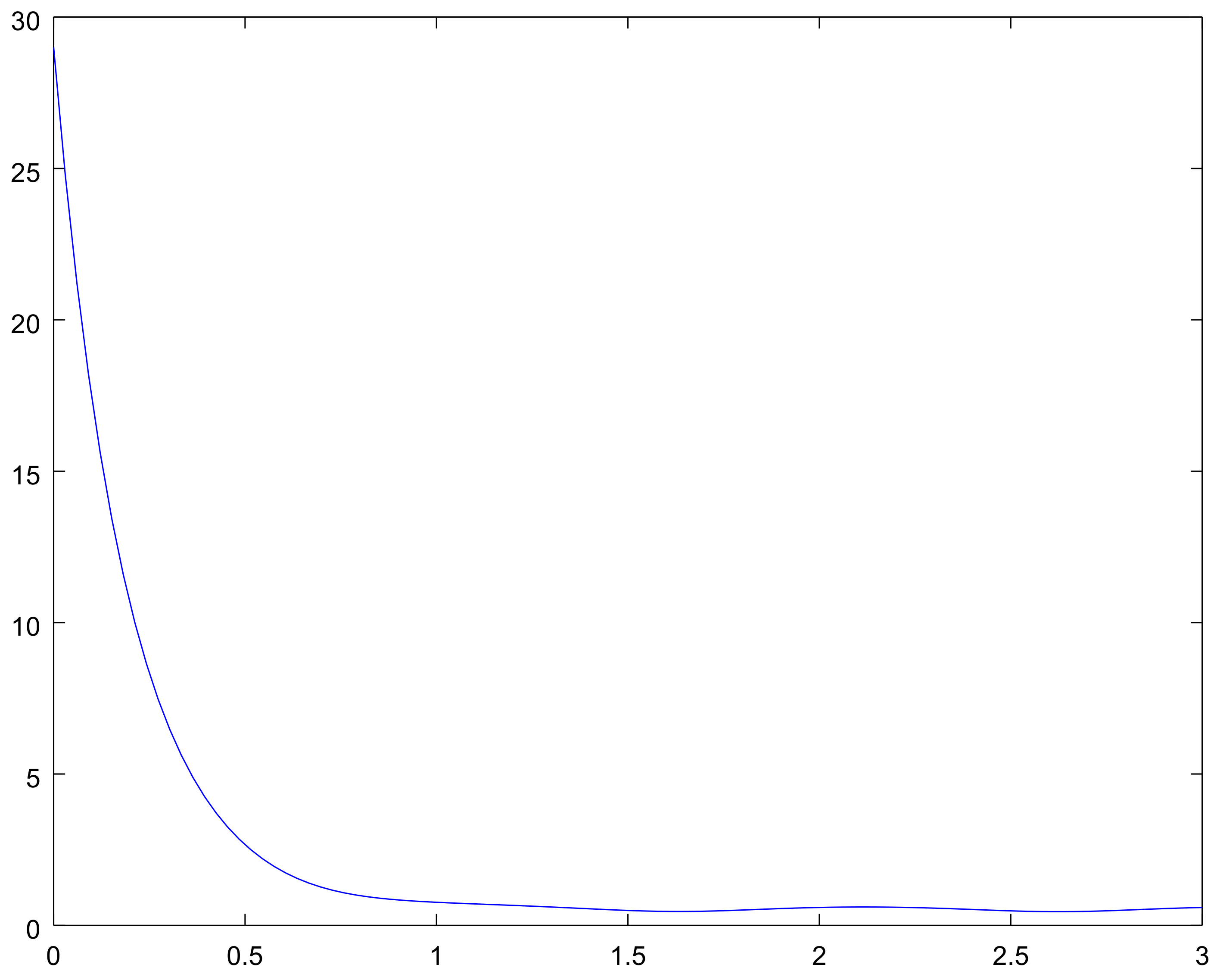
Consider the diagonal matrix $D=diag(d_0,d_1,d_2,d_3,\cdots )$, with entries of the increasing sequence $\{d_n\}$, where $d_0=1$, and the corresponding space of sequences $l_{1D}=\{\mathbf{z}={(p_0,p_1,p_2,\dots )}^T\}$ such that ${\parallel \mathbf{z}\parallel }_{1D}={\parallel D\mathbf{z}\parallel }_1<\infty$.

Then one can estimate the logarithmic norm of operator $B(t)$ in $l_{1D}$ space.

According to the general approach, we obtain the matrix $DB(t)D^{-1}=\left(\begin{array}{ccccccccc}{a}_{00}-\xi & ({\mu }_{1,0,1}+{\xi }_{0,1}-\xi )\frac{d_0}{d_1}& ({\mu }_{2,1,0}+{\xi }_{1,0}-\xi )\frac{d_0}{d_2}& ({\xi }_{0,2}-\xi )\frac{d_0}{d_3}& ({\xi }_{1,1}-\xi )\frac{d_0}{d_4}& ({\xi }_{2,0}-\xi )\frac{d_0}{d_5}& ({\xi }_{0,3}-\xi )\frac{d_0}{d_6}& ({\xi }_{1,2}-\xi )\frac{d_0}{d_7}& \cdots \\ {\lambda }_{1,0,0}\frac{d_1}{d_0}& a_{11}& 0& {\mu }_{1,0,2}\frac{d_1}{d_3}& {\mu }_{2,1,1}\frac{d_1}{d_4}& 0& 0& 0& \cdots \\ {\lambda }_{2,0,0}\frac{d_2}{d_0}& 0& a_{22}& 0& {\mu }_{1,1,1}\frac{d_2}{d_4}& {\mu }_{2,2,0}\frac{d_2}{d_5}& 0& 0& \cdots \\ 0& {\lambda }_{1,0,1}\frac{d_3}{d_1}& 0& a_{33}& 0& 0& {\mu }_{1,0,3}\frac{d_3}{d_6}& {\mu }_{2,1,2}\frac{d_3}{d_7}& \cdots \\ 0& {\lambda }_{2,0,1}\frac{d_4}{d_1}& {\lambda }_{1,1,0}\frac{d_4}{d_2}& 0& a_{44}& 0& 0& {\mu }_{1,1,2}\frac{d_4}{d_7}& \cdots \\ 0& 0& {\lambda }_{2,1,0}\frac{d_5}{d_2}& 0& 0& a_{55}& 0& 0& \cdots \\ 0& 0& 0& {\lambda }_{1,0,2}\frac{d_6}{d_3}& 0& 0& a_{66}& 0& \cdots \\ \cdots & \cdots & \cdots & \cdots & \cdots & \cdots & \cdots \end{array}\right),$ where $a_{ii}(t)=-{\sum }_i{a}_{i,j}(t)$.

Consider now the logarithmic norm

$$\begin{array}{c}\hfill \gamma {\left(B(t)\right)}_{1D}=\gamma {\left(DB(t)D^{-1}\right)}_1.\end{array}$$

(20)

Let us make the correspondence between the column number of matrix $DB(t)D^{-1}$ and the number of zeros under the main diagonal in this column (till the first nonzero element). Then we obtain the arithmetic progression $\left\{a_i\right\}$:

$$\begin{array}{cccccccccccccccccccccc}{a}_1& a_2& a_3& a_4& a_5& a_6& a_7& a_8& a_9& a_{10}& a_{11}& a_{12}& a_{13}& a_{14}& a_{15}& a_{16}& a_{17}& a_{18}& a_{19}& a_{20}& a_{21}& \cdots \\ 1& 2& 3& 4& 5& 6& 7& 8& 9& 10& 11& 12& 13& 14& 15& 16& 17& 18& 19& 20& 21& \cdots \\ 1& 1& 2& 2& 2& 3& 3& 3& 3& 4& 4& 4& 4& 4& 5& 5& 5& 5& 5& 5& 6& \cdots \end{array}$$

We compose the sequence $\left\{b_i\right\}$ of the number of identical entries of the third line: $2,3,4,5,6,\cdots$. Note that ${\sum }_{i=1}^N{b}_i$ is equal to the last $a_k$, corresponding to the number of zeros N in the k-th column.

Then the sum of the first N elements of sequence $\left\{b_i\right\}$ is approximately equal to the number of the column $a_n=n$:

$$\left(2b_1+(N-1)\right)N\approx 2a_n=2n.$$

Knowing the column number n, one can find the formula for the number of zeros N under the main diagonal in this column till the first nonzero element. We note that the number of zeros over the diagonal till ${\mu }_{1,i,j}$ is one less.

If N is not an integer, we must take the nearest right to N an integer.

One can see that columns $2,5,9,14,\dots$ (these columns correspond to sums ${\sum }_{i=1}^j{b}_i$ and integer N) contain death rates ${\mu }_{2,i,j}(t)$ only, and columns $3,6,10,15,\dots$ contain death rates ${\mu }_{1,i,j}(t)$ only, and all other columns contain the both death intensities.

Consider the following quantities:

for $n=0$

$$\begin{array}{c}{\alpha }_n\left(t\right)={\lambda }_{1,0,0}(t)+{\lambda }_{2,0,0}(t)+\xi (t)-{\lambda }_{1,0,0}(t)\frac{d_1}{d_0}-{\lambda }_{2,0,0}(t)\frac{d_2}{d_0},\end{array}$$

for $n=1$

$$\begin{array}{c}{\alpha }_n\left(t\right)={\lambda }_{1,0,1}(t)+{\lambda }_{2,0,1}(t)+{\mu }_{1,0,1}(t)+{\xi }_1(t)-{\lambda }_{1,0,1}(t)\frac{d_3}{d_1}-{\lambda }_{2,0,1}(t)\frac{d_4}{d_1}-({\mu }_{1,0,1}(t)+{\xi }_1(t)-\xi (t))\frac{d_0}{d_1},\end{array}$$

for $n=2$

$$\begin{array}{c}{\alpha }_n\left(t\right)={\lambda }_{1,1,0}(t)+{\lambda }_{2,1,0}(t)+{\mu }_{2,1,0}(t)+{\xi }_2(t)-{\lambda }_{1,1,0}(t)\frac{d_4}{d_2}-{\lambda }_{2,1,0}(t)\frac{d_5}{d_2}-({\mu }_{2,1,0}(t)+{\xi }_2(t)-\xi (t))\frac{d_0}{d_2},\end{array}$$

for integer $\frac{-3+\sqrt{9+8n}}{2}$:

$$\begin{array}{c}{\alpha }_n\left(t\right)={\lambda }_{1,s^{-1}\left(n\right)}(t)+{\lambda }_{2,s^{-1}\left(n\right)}(t)+{\mu }_{2,s^{-1}\left(n\right)}(t)+{\xi }_{s(i,j)}(t)-{\lambda }_{1,s^{-1}\left(n\right)}(t)\frac{d_{n+N+1}}{d_n}-{\lambda }_{2,s^{-1}\left(n\right)}(t)\frac{d_{n+N+2}}{d_n}\hfill \\ -{\mu }_{2,s^{-1}\left(n\right)}(t)\frac{d_{n-N-1}}{d_n}-({\xi }_{s(i,j)}(t)-\xi (t))\frac{d_0}{d_n},N=\frac{-3+\sqrt{9+8n}}{2},\hfill \end{array}$$

for integer $\frac{-3+\sqrt{9+8(n-1)}}{2}$:

$$\begin{array}{c}{\alpha }_n\left(t\right)={\lambda }_{1,s^{-1}\left(n\right)}(t)+{\lambda }_{2,s^{-1}\left(n\right)}(t)+{\mu }_{1,s^{-1}\left(n\right)}(t)+{\xi }_{s(i,j)}(t)-{\lambda }_{1,s^{-1}\left(n\right)}(t)\frac{d_{n+N+1}}{d_n}-{\lambda }_{2,s^{-1}\left(n\right)}(t)\frac{d_{n+N+2}}{d_n}\hfill \\ -{\mu }_{1,s^{-1}\left(n\right)}(t)\frac{d_{n-N}}{d_n}-({\xi }_{s(i,j)}(t)-\xi (t))\frac{d_0}{d_n},N=⌈\frac{-3+\sqrt{9+8n}}{2}⌉,\hfill \end{array}$$

in other cases:

$$\begin{array}{c}{\alpha }_n\left(t\right)={\lambda }_{1,s^{-1}\left(n\right)}(t)+{\lambda }_{2,s^{-1}\left(n\right)}(t)+{\mu }_{1,s^{-1}\left(n\right)}(t)+{\mu }_{2,s^{-1}\left(n\right)}(t)+{\xi }_{s(i,j)}(t)-{\lambda }_{1,s^{-1}\left(n\right)}(t)\frac{d_{n+N+1}}{d_n}\hfill \\ -{\lambda }_{2,s^{-1}\left(n\right)}(t)\frac{d_{n+N+2}}{d_n}-{\mu }_{1,s^{-1}\left(n\right)}(t)\frac{d_{n-N}}{d_n}-{\mu }_{2,s^{-1}\left(n\right)}(t)\frac{d_{n-N-1}}{d_n}\hfill \\ -({\xi }_{s(i,j)}(t)-\xi (t))\frac{d_0}{d_n},N=⌈\frac{-3+\sqrt{9+8n}}{2}⌉.\hfill \end{array}$$

Then the following algorithm helps us to correlate the number n and pair $(i,j)$:

(1) $n_1=n-1$,

(2) $n_2=n_1-2$,

⋯

(k) $n_k=n_{k-1}-k$, while $n_k>0$,

(k+1) $i=n_k,j=k-n_k$.

We obtain

$$\gamma {\left(B(t)\right)}_{1D}=-\underset{t}{inf}{\alpha }_n(t)=-\alpha (t).$$

(21)

Therefore, for all $0\le s\le t$ we have the bound for the corresponding Cauchy operator:

$${\parallel V(t,s)\parallel }_{1D}\le e^{-\underset{s}{\overset{t}{\int }}\alpha (\tau )d\tau },$$

(22)

and the following statement.

Theorem 3.

Let for some sequence $\left\{d_i\right\}$ we have the condition

$${\int }_0^{\infty }\alpha (t)dt=\infty .$$

(23)

Then the process $\mathbf{X}(t)$ is weakly ergodic and the following bound of the rate of convergence is correct:

$$\begin{array}{c}\hfill {∥{\mathbf{p}}^{\ast }(t)-{\mathbf{p}}^{\ast \ast }(t)∥}_{1D}\le e^{-\underset{0}{\overset{t}{\int }}\alpha (\tau )d\tau }{∥{\mathbf{p}}^{\ast }(0)-{\mathbf{p}}^{\ast \ast }(0)∥}_{1D},\end{array}$$

(24)

for any initial conditions ${\mathbf{p}}^{\ast }(0),{\mathbf{p}}^{\ast \ast }(0)$ and for all $t\ge 0$.

Mathematical expectations for both processes $X_1(t)$ and $X_2(t)$ can be obtained using formulas:

$$\begin{array}{c}\hfill E_1(t)=1(p_2+p_4+p_7+\dots )+2(p_5+p_8+p_{12}+\cdots )+\dots \\ \hfill =1(p_{10}+p_{11}+p_{12}+\dots )+2(p_{20}+p_{21}+p_{22}+\cdots )+\dots \end{array}$$

(25)

and

$$\begin{array}{c}\hfill E_2(t)=1(p_1+p_4+p_8+\dots )+2(p_3+p_7+p_{12}+\cdots )+\dots \\ \hfill =1(p_{01}+p_{11}+p_{21}+\dots )+2(p_{02}+p_{12}+p_{22}+\cdots )+\dots .\end{array}$$

(26)

Let us now introduce a process $N(t)=|\mathbf{X}(t)|=X_1(t)+X_2(t)$, that is the number of all particles at the moment t.

Then one has for the mathematical expectation (the mean) of this process the following equality:

$$\begin{array}{c}\hfill E_N(t)=1(p_{01}+p_{10})+2(p_{02}+p_{11}+p_{20})+3(p_{03}+p_{12}+p_{21}+p_{30})+\cdots )+\dots \\ \hfill =1(p_1+p_2)+2(p_3+p_4+p_5)+3(p_6+p_7+p_8+p_9)+\dots =E_1(t)+E_2(t).\end{array}$$

(27)

We note that for $W={inf}_{i\ge 0}\frac{d_i}{i}$ the next inequality holds

$$E_N(t)=1(p_1+p_2)+2(p_3+p_4+p_5)+3(p_6+p_7+p_8+p_9)+\dots \le \sum _{i\ge 1}i{p}_i\le \frac{1}{W}\sum _{i\ge 1}{d}_i{p}_i=\frac{{\parallel p(t)\parallel }_{1D}}{W}.$$

Denote by $E_N(t,k)=E(|X(t)|/|X(0)|=k)$ the conditional expected number of all particles in the system at instant t, provided that initially (at instant $t=0$) k particles of both types were present in the system.

Corollary 2.

Let the condition (23) hold and there is a sequence $\left\{d_i\right\}$ such that $W>0$, then the process $N(t)$ has the limiting mean ${\varphi }_N(t)=E_N(t,0)$, and for any j and all $t\ge 0$ the following bound of the rate of convergence is correct:

$$|E_N(t,j)-E_N(t,0)|\le \frac{1+d_j}{W}{e}^{-\underset{0}{\overset{t}{\int }}\alpha (\tau )d\tau }.$$

(28)

Applying in addition the condition that the perturbations of the intensity matrix are small enough in the corresponding norm, that is $\parallel \widehat{A}{(t)\parallel }_{1D}\le \epsilon ,$ one can also obtain $\parallel \widehat{B}{(t)\parallel }_{1D}\le \epsilon .$

We assume here that the process $\mathbf{X}(t)$ is exponentially ergodic in $l_{1D}$-norm, that is for some positive $M_1,a_1$ and for all s, t, $0\le s\le t$ the following inequality holds:

$$e^{-{\int }_s^t\alpha (u)du}\le M_1{e}^{-a_1(t-s)}.$$

(29)

Here we apply the approach from [18].

One can rewrite the original system for the unperturbed process in the form:

$$\frac{d\mathbf{p}}{dt}=\overline{\mathbf{B}}(t)\mathbf{p}(t)+\overline{\mathbf{f}}(t)+\widehat{\mathbf{B}}(t)\mathbf{p}(t)+\widehat{\mathbf{f}}(t).$$

(30)

Then

$$\mathbf{p}(t)=\overline{V}(t,0)\mathbf{p}(0)+{\int }_0^t\overline{V}(t,\tau )\overline{\mathbf{f}}(\tau )d\tau +{\int }_0^t\overline{V}(t,\tau )\widehat{B}(\tau )p(\tau )$$

(31)

and

$$\overline{\mathbf{p}}(t)=\overline{V}(t,0)\overline{\mathbf{p}}(0)+{\int }_0^t\overline{V}(t,\tau )\overline{\mathbf{f}}(\tau )d\tau .$$

(32)

Therefore, in any norm for any initial conditions we have the correct bound:

$$∥\mathbf{p}(t)-\overline{\mathbf{p}}(t)∥\le {\int }_0^t\parallel \overline{V}(t,\tau )\parallel \left(\parallel \widehat{B}(\tau )\parallel \parallel \mathbf{p}(\tau )\parallel +\parallel \widehat{\mathbf{f}}(\tau )\parallel \right)d\tau .$$

(33)

Then we have the following inequality for the logarithmic norm:

$$\begin{array}{c}\hfill \gamma {(\overline{B}(t))}_{1D}\le \gamma {(DB(t)D^{-1})}_1+{\parallel \widehat{B}(t)\parallel }_{1D}\le -\alpha (t)+\epsilon .\end{array}$$

(34)

On the other hand, one can obtain the estimation using inequality (29):

$$\begin{array}{c}\hfill {\parallel \mathbf{p}(t)\parallel }_{1D}\le {\parallel V(t)\mathbf{p}(0)\parallel }_{1D}+\underset{0}{\overset{t}{\int }}{\parallel V(t,\tau )\mathbf{f}(\tau )d\tau \parallel }_{1D}\le \\ \hfill \le M_1{e}^{-a_{1}t}{\parallel \mathbf{p}(0)\parallel }_{1D}+\frac{L{M}_1}{a_1}\end{array}$$

(35)

for any initial condition $\mathbf{p}(0)$. Moreover, $\parallel \widehat{\mathbf{f}}{(\tau )\parallel }_{1D}\le \epsilon$.

Then using bound (33), we have

$$\begin{array}{c}\hfill \parallel \mathbf{p}(t)-\overline{\mathbf{p}}{(t)\parallel }_{1D}\le {\int }_0^t{e}^{-{\int }_{\tau }^t(\alpha (u)-\epsilon )du}\left(\epsilon \left(M_1{e}^{-a_1\tau }{\parallel \mathbf{p}(0)\parallel }_{1D}+\frac{L{M}_1}{a_1}\right)+\epsilon \right)d\tau \le \\ \hfill \le o(1)+\frac{\epsilon M_1(1+L{M}_1/a_1)}{a_1-\epsilon }.\end{array}$$

Therefore, the following statement is correct.

Theorem 4.

Let inequalities (12) and (29) hold for any initial condition $\mathbf{p}(0)\in l_{1D}$ and for all $t\ge 0$, then we have

$${∥\mathbf{p}(t)-\overline{\mathbf{p}}(t)∥}_{1D}\le M_1\epsilon \left(\frac{L{M}_1+a_1}{a_1(a_1-\epsilon )}+M_{1}t{e}^{-(a_1-\epsilon )t}{\parallel \mathbf{p}(0)\parallel }_{1D}\right),$$

(36)

and

$$\underset{t\to \infty }{lim\; sup}{∥\mathbf{p}(t)-\overline{\mathbf{p}}(t)∥}_{1D}\le \frac{M_1\epsilon (L{M}_1+a_1)}{a_1(a_1-\epsilon )}.$$

(37)

Corollary 3.

Let in addition the sequence be increasing fast enough, such that $W>0$, then for any j, $t\ge 0$ we have

$$\underset{t\to \infty }{lim\; sup}|E_N(t)-{\overline{E}}_N(t)|\le \frac{M_1\epsilon (L{M}_1+a_1)}{W{a}_1(a_1-\epsilon )}.$$

(38)

4. Examples

Example 1.

Let ${\lambda }_{1,i,j}(t)={\lambda }_{2,i,j}(t)=2+sin2\pi t,i,j\ge 0$, ${\mu }_{2,0,1}(t)=1+cos2\pi t$, ${\mu }_{1,1,0}(t)=2(1+cos2\pi t)$, and other ${\mu }_{1,i,j}(t)={\mu }_{2,i,j}(t)=3(1+cos2\pi t)$, and let catastrophe intensities be ${\xi }_{i,j}(t)=5$. Put $\epsilon ={10}^{-6}$.

Choose $d_n=1+\frac{n}{10}$, then $\alpha (t)={\alpha }_0(t)-\frac{2}{3}=\frac{56}{10}-\frac{3}{10}sin2\pi t$, $a=5,M=1,a_1=3.8,M_1=1.1$, W = 1/10.

We obtain now the following bounds

$$|E_N(t,1)-E_N(t,0)|\le 3.4·{10}^{-4},t\ge 4,$$

(39)

$$\underset{t\to \infty }{lim\; sup}∥\mathbf{p}(t)-\overline{\mathbf{p}}(t)∥\le 2·{10}^{-4},$$

(40)

$$\underset{t\to \infty }{lim\; sup}\left|E_N(t,0)-{\overline{E}}_N(t,0)\right|\le 0.023.$$

(41)

The values of ${\alpha }_n(t)$ are shown in Figure 2. The mean for the process $N(t)$ on the interval $t\in [0,3]$ for different initial conditions are shown in Figure 3, Figure 4, Figure 5 and Figure 6, and the bounds for the limiting perturbed mean is shown in Figure 7.

Example 2.

Let now ${\lambda }_{1,i,j}(t)={\lambda }_{2,i,j}(t)=2+cos2\pi t,i,j\ge 0$, ${\mu }_{1,i,j}(t)=min(1+i·j,3)(1+cos2\pi t),$$i\ge 1,j\ge 0$, ${\mu }_{2,i,j}(t)=min(1+i·j,3)(1+cos2\pi t),i\ge 0,j\ge 1$, and let the catastrophe rates be ${\xi }_{i,j}(t)=5$. Let $\epsilon ={10}^{-3}$.

Put $d_n=1+\frac{n}{10}$, then $\alpha (t)={\alpha }_9(t)-\frac{1}{7}=\frac{548}{133}+\frac{4}{19}sin2\pi t-\frac{9}{19}cos2\pi t$, $a=5,M=1,a_1=4.12,$$M_1=1.2,W=1/10$.

Then we obtain

$$|E_N(t,1)-E_N(t,0)|\le 9.4·{10}^{-4},t\ge 2,$$

(42)

$$\underset{t\to \infty }{lim\; sup}∥\mathbf{p}(t)-\overline{\mathbf{p}}(t)∥\le 2·{10}^{-4},$$

(43)

$$\underset{t\to \infty }{lim\; sup}\left|E_N(t,0)-{\overline{E}}_N(t,0)\right|\le 0.021.$$

(44)

The values of ${\alpha }_n(t)$ are shown in Figure 8.

The mean for the process $N(t)$ on the interval $t\in [0,3]$ for different initial conditions are shown in Figure 9, Figure 10, Figure 11 and Figure 12, and the bounds for the limiting perturbed mean is shown in Figure 13.

Remark 1.

These graphs give us the additional information on the considered examples. Namely, Figure 2 and Figure 8 show the bounding on the rate of convergence, see Equation (21) for Examples 1, 2 respectively, in Figure 3, Figure 4, Figure 5 and Figure 6 and Figure 9, Figure 10, Figure 11 and Figure 12 one can see the mathematical expectation of the number of all particles at the moment t until the stationary behaviour. Finally, the limiting behaviour of the limiting mathematical expectation of the number of all particles for the perturbed process is shown in Figure 7 and Figure 13.

References

1. Di Crescenzo, A.; Giorno, V.; Nobile, A.G.; Ricciardi, L.M. On the M/M/1 queue with catastrophes and its continuous approximation. Queueing Syst. 2003, 43, 329–347. [Google Scholar] [CrossRef]
2. Di Crescenzo, A.; Giorno, V.; Nobile, A.G.; Ricciardi, L.M. A note on birth-death processes with catastrophes. Stat. Probab. Lett. 2008, 78, 2248–2257. [Google Scholar] [CrossRef]
3. Di Crescenzo, A.; Giorno, V.; Kumar, B.K.; Nobile, A.G. A double-ended queue with catastrophes and repairs, and a jump-diffusion approximation. Methodol. Comput. Appl. Probab. 2012, 14, 937–954. [Google Scholar] [CrossRef]
4. Dharmaraja, S.; Di Crescenzo, A.; Giorno, V.; Nobile, A.G. A continuous-time Ehrenfest model with catastrophes and its jump-diffusion approximation. J. Stat. Phys. 2015, 161, 326–345. [Google Scholar] [CrossRef]
5. Dudin, A.; Nishimura, S. A BMAP/SM/1 queueing system with Markovian arrival input of disasters. J. Appl. Probab. 1999, 36, 868–881. [Google Scholar] [CrossRef]
6. Dudin, A.; Karolik, A. BMAP/SM/1 queue with Markovian input of disasters and non-instantaneous recovery. Perform. Eval. 2001, 45, 19–32. [Google Scholar] [CrossRef]
7. Dudin, A.; Semenova, O. A stable algorithm for stationary distribution calculation for a BMAP/SM/1 queueing system with Markovian arrival input of disasters. J. Appl. Probab. 2004, 41, 547–556. [Google Scholar] [CrossRef]
8. Do, T.V.; Papp, D.; Chakka, R.; Sztrik, J.; Wang, J. M/M/1 retrial queue with working vacations and negative customer arrivals. Int. J. Adv. Intell. Paradig. 2014, 6, 52–65. [Google Scholar] [CrossRef]
9. Chen, A.Y.; Renshaw, E. The M/M/1 queue with mass exodus and mass arrives when empty. J. Appl. Prob. 1997, 34, 192–207. [Google Scholar] [CrossRef]
10. Chen, A.Y.; Renshaw, E. Markov bulk-arriving queues with state-dependent control at idle time. Adv. Appl. Prob. 2004, 36, 499–524. [Google Scholar] [CrossRef]
11. Chen, A.Y.; Pollett, P.; Li, J.P.; Zhang, H.J. Markovian bulk-arrival and bulk-service queues with state-dependent control. Queueing Syst. 2010, 64, 267–304. [Google Scholar] [CrossRef]
12. Li, J.; Chen, A. The Decay Parameter and Invariant Measures for Markovian Bulk-Arrival Queues with Control at Idle Time. Methodol. Comput. Appl. Probab. 2013, 15, 467–484. [Google Scholar]
13. Zhang, L.; Li, J. The M/M/c queue with mass exodus and mass arrivals when empty. J. Appl. Probab. 2015, 52, 990–1002. [Google Scholar] [CrossRef]
14. Zeifman, A.; Korotysheva, A.; Satin, Y.; Shorgin, S. On stability for nonstationary queueing systemswith catastrophes. Inform. Appl. 2010, 4, 9–15. [Google Scholar]
15. Zeifman, A.; Korotysheva, A.; Panfilova, T.; Shorgin, S. Stability bounds for some queueing systems with catastrophes. Inform. Appl. 2011, 5, 27–33. [Google Scholar]
16. Zeifman, A.; Korotysheva, A. Perturbation Bounds for Mt/Mt/N Queue with Catastrophes. Stoch. Model. 2012, 28, 49–62. [Google Scholar] [CrossRef]
17. Zeifman, A.; Satin, Y.; Panfilova, T. Limiting characteristics for finite birth-death-catastrophe processes. Mater. Biosci. 2013, 245, 96–102. [Google Scholar] [CrossRef] [PubMed]
18. Zeifman, A.; Satin, Y.; Korotysheva, A.; Korolev, V.; Shorgin, S.; Razumchik, R. Ergodicity and perturbation bounds for inhomogeneous birth and death processes with additional transitions from and to origin. Int. J. Appl. Math. Comput. Sci. 2015, 25, 787–802. [Google Scholar] [CrossRef]
19. Zeifman, A.; Satin, Y.; Korotysheva, A.; Korolev, V.; Bening, V. On a class of Markovian queuing systems described by inhomogeneous birth-and-death processes with additional transitions. Dokl. Math. 2016, 94, 502–505. [Google Scholar] [CrossRef]
20. Zeifman, A.; Korotysheva, A.; Satin, Y.; Kiseleva, K.; Korolev, V.; Shorgin, S. Ergodicity and uniform in time truncation bounds for inhomogeneous birth and death processes with additional transitions from and to origin. Stoch. Model. 2017, 33, 598–616. [Google Scholar] [CrossRef]
21. Giorno, V.; Nobile, A.; Spina, S. On some time non-homogeneous queueing systems with catastrophes. Appl. Math. 2014, 245, 220–234. [Google Scholar] [CrossRef]
22. Zeifman, A.; Korotysheva, A.; Satin, Y.; Kiseleva, K.; Korolev, V.; Shorgin, S. Bounds for Markovian Queues with Possible Catastrophes. In Proceedings of the 31th European Conference on Modeling and Simulation, Budapest, Hungary, 23–26 May 2017; pp. 628–634. [Google Scholar]
23. Daleckii, J.L.; Krein, M.G. Stability of solutions of differential equations in Banach space (No. 43). Am. Math. Soc. 2002, 53, 34–36. [Google Scholar]
24. Zeifman, A.; Satin, Y.; Chegodaev, A. On nonstationary queueing systems with catastrophes. Inform. Appl. 2009, 3, 47–54. [Google Scholar]
25. Mitrophanov, A.Y. Stability and exponential convergence of continuous-time Markov chains. J. Appl. Prob. 2003, 40, 970–979. [Google Scholar] [CrossRef]
Figure 1. Transition rate diagram.
Mathematics 06 00080 g001
Figure 2. The values of several α n ( t ) for Example 1.
Mathematics 06 00080 g002
Figure 3. The mean E N ( t , 0 ) on the interval t [ 0 , 3 ] with initial condition X ( t ) = ( 0 , 0 ) for Example 1.
Mathematics 06 00080 g003
Figure 4. The mean E N ( t , 29 ) on the interval t [ 0 , 3 ] with initial condition X ( t ) = ( 0 , 29 ) for Example 1.
Mathematics 06 00080 g004
Figure 5. The mean E N ( t , 29 ) on the interval t [ 0 , 3 ] with initial condition X ( t ) = ( 14 , 15 ) for Example 1.
Mathematics 06 00080 g005
Figure 6. The mean E N ( t , 29 ) on the interval t [ 0 , 3 ] with initial condition X ( t ) = ( 29 , 0 ) for Example 1.
Mathematics 06 00080 g006
Figure 7. The limiting perturbed mean for t [ 2 , 3 ] for Example 1.
Mathematics 06 00080 g007
Figure 8. The values of several α n ( t ) for Example 2.
Mathematics 06 00080 g008
Figure 9. The mean E N ( t , 0 ) on the interval t [ 0 , 3 ] with initial condition X ( t ) = ( 0 , 0 ) for Example 2.
Mathematics 06 00080 g009
Figure 10. The mean E N ( t , 29 ) on the interval t [ 0 , 3 ] with initial condition X ( t ) = ( 0 , 29 ) for Example 2.
Mathematics 06 00080 g010
Figure 11. The mean E N ( t , 29 ) on the interval t [ 0 , 3 ] with initial condition X ( t ) = ( 14 , 15 ) for Example 2.
Mathematics 06 00080 g011
Figure 12. The mean E N ( t , 29 ) on the interval t [ 0 , 3 ] with initial condition X ( t ) = ( 0 , 29 ) for Example 2.
Mathematics 06 00080 g012
Figure 13. The limiting perturbed mean for t [ 2 , 3 ] for Example 2.
Mathematics 06 00080 g013