Effects of Viral and Cytokine Delays on Dynamics of Autoimmunity


Abstract
1. Introduction
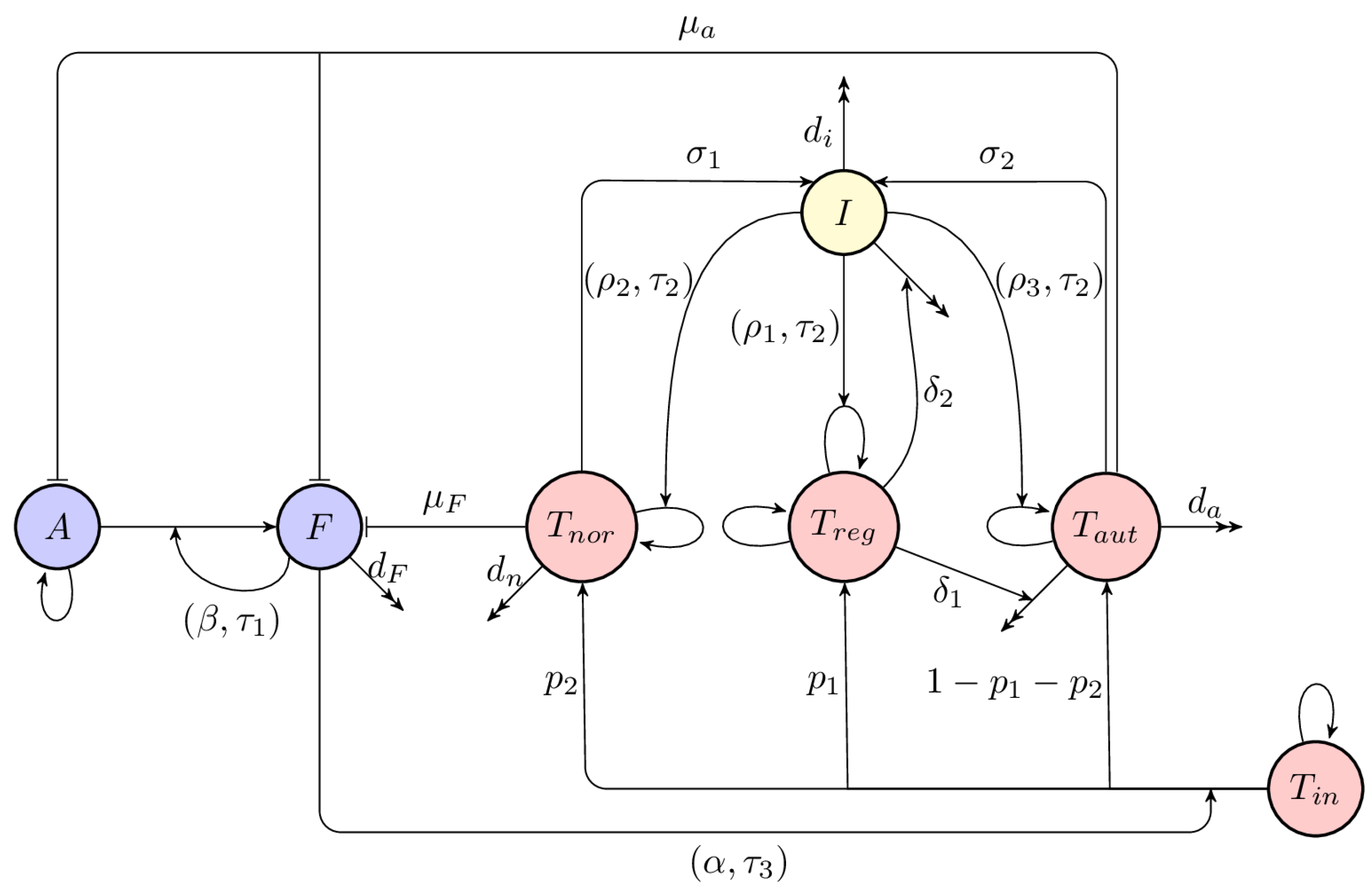
2. Model Derivation
3. Stability Analysis of the Steady States
3.1. Stability Analysis of the Disease-Free Steady State
3.2. Stability Analysis of the Death, Autoimmune and Chronic Steady States
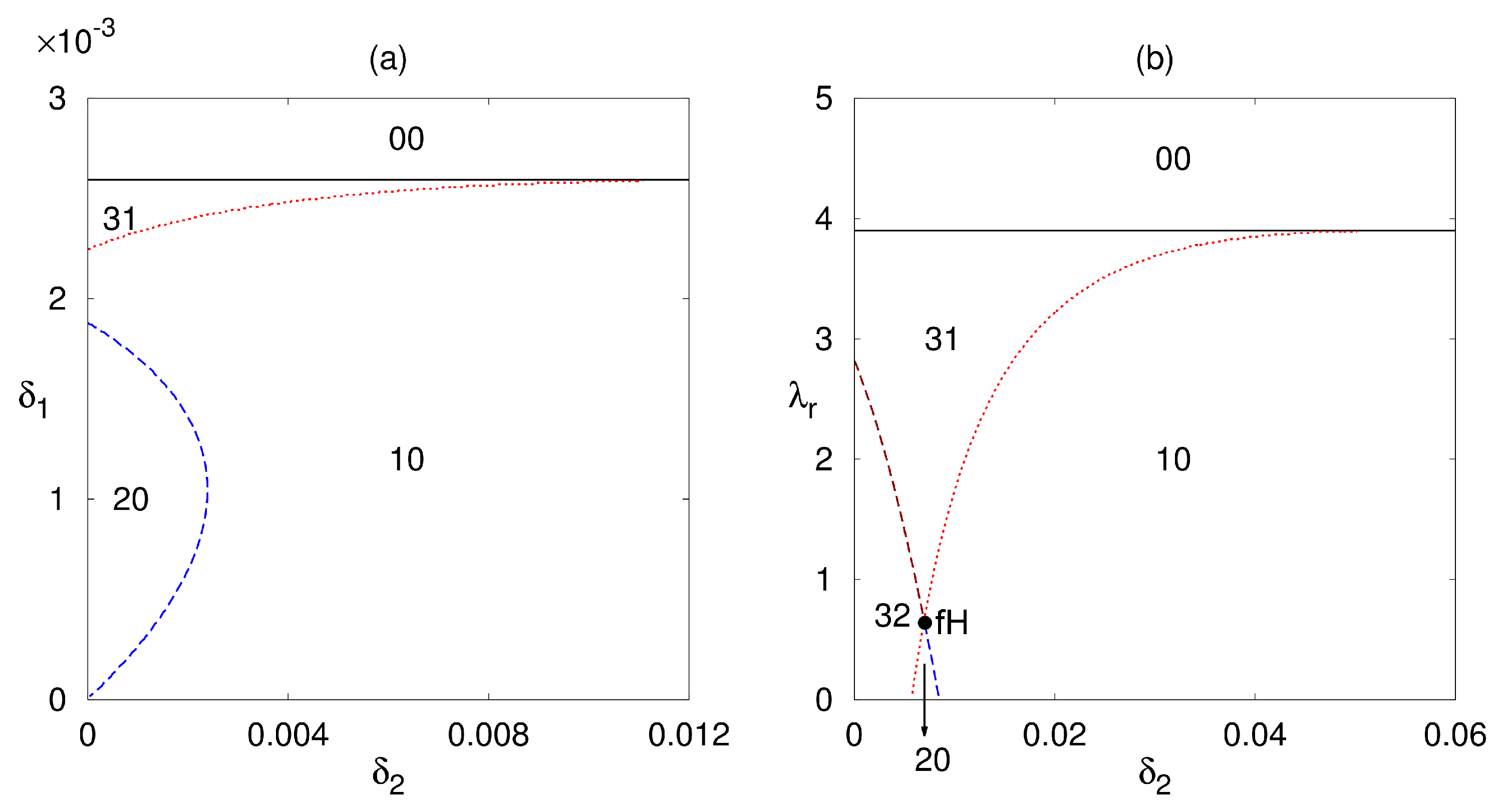
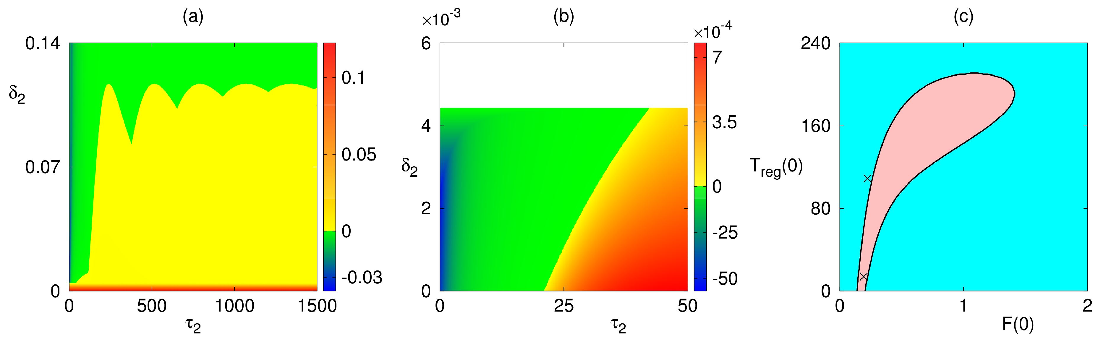
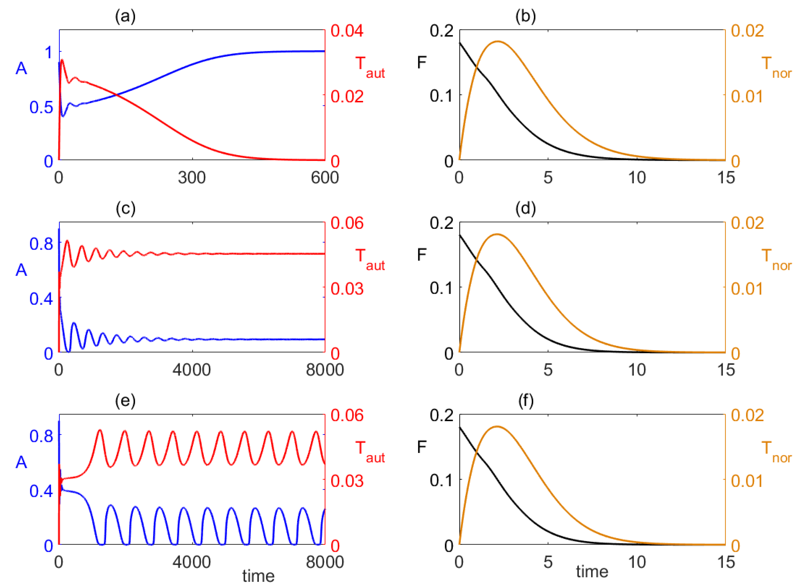
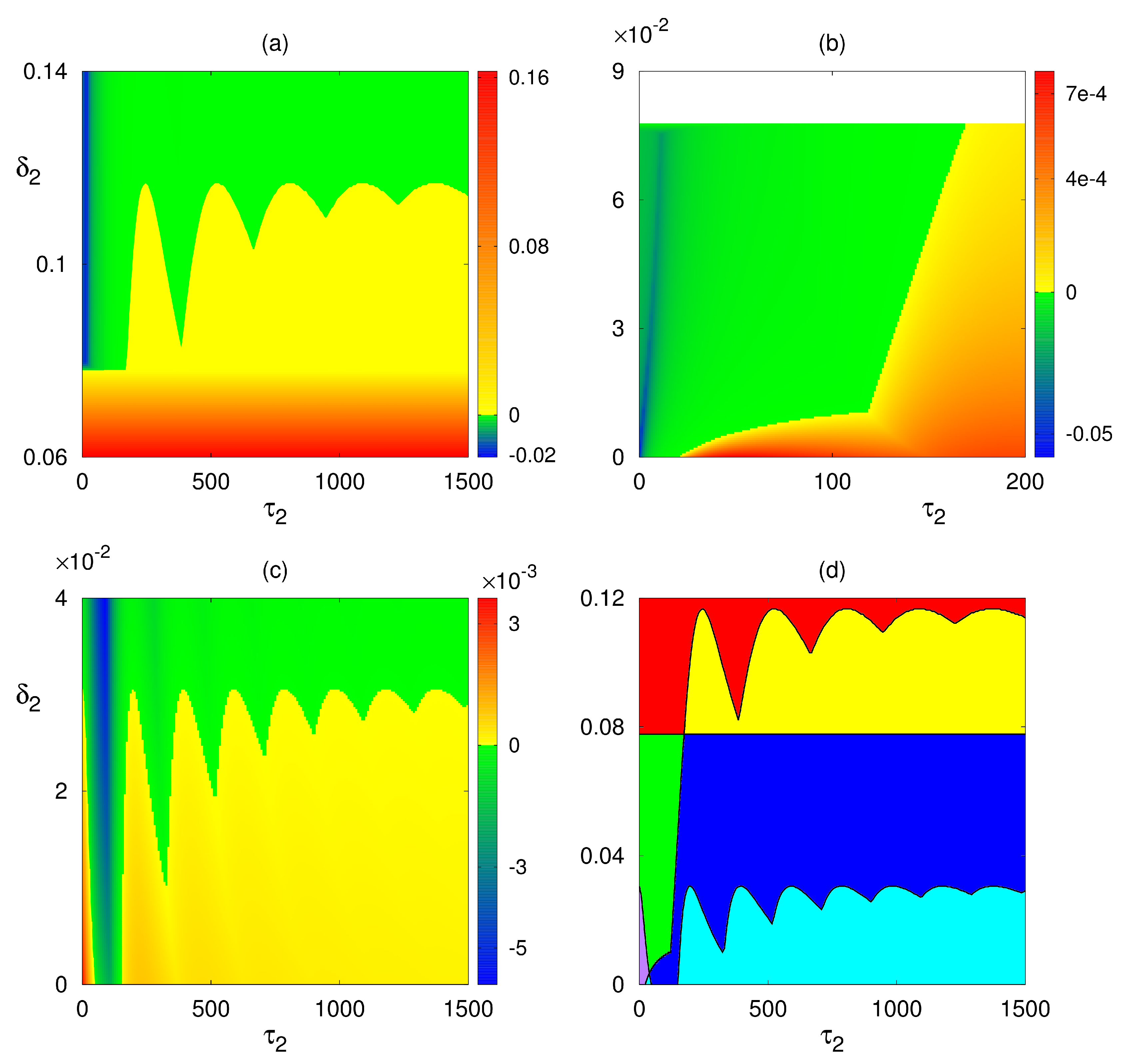
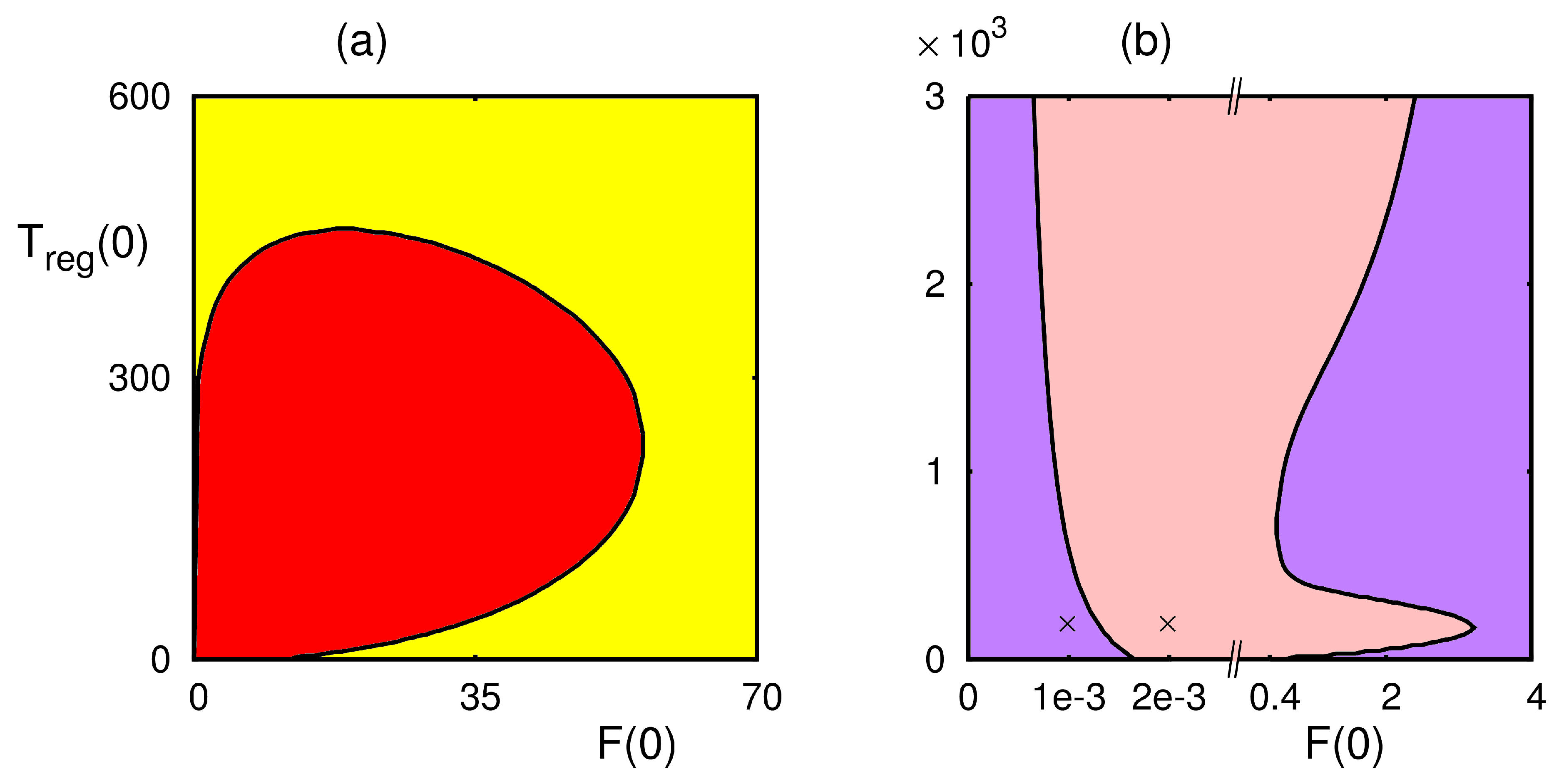
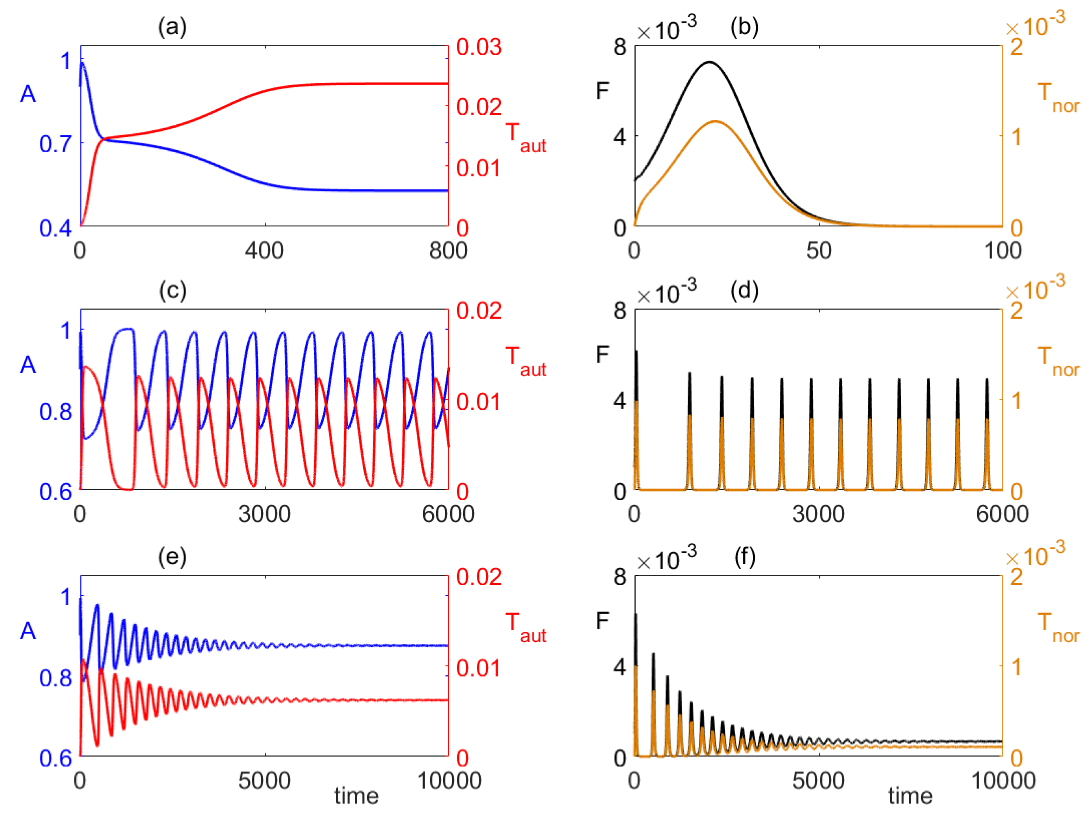
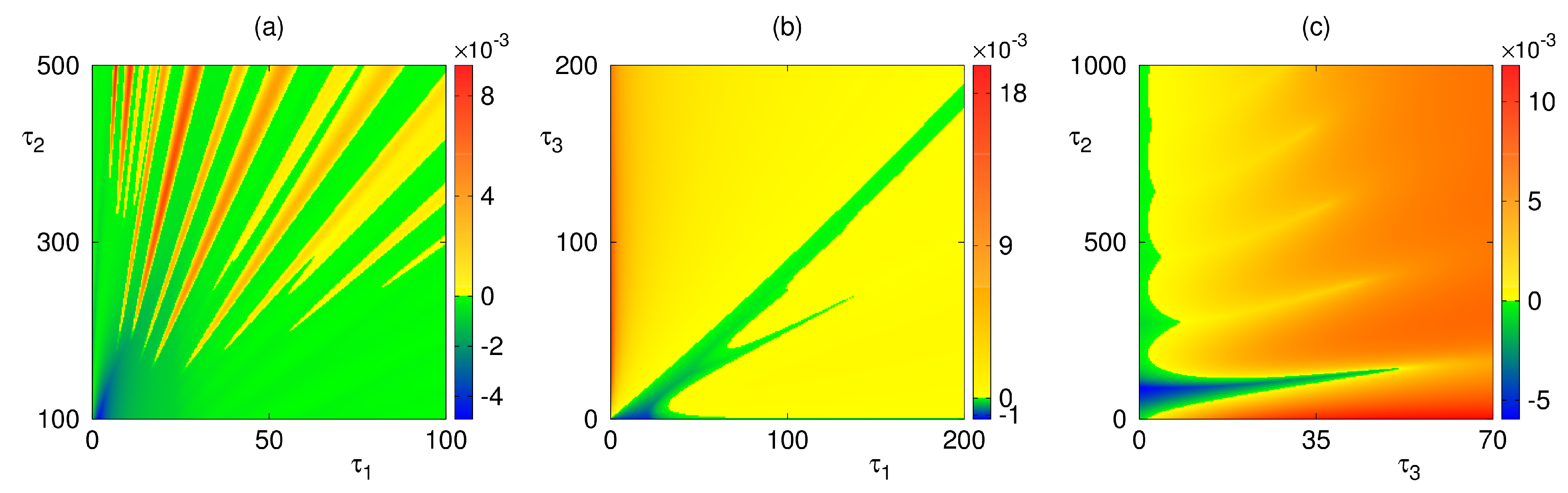
4. Numerical Stability Analysis and Simulations
5. Conclusions
Author Contributions
Acknowledgments
Conflicts of Interest
Appendix A
References
- Mason, D. A very high level of crossreactivity is an essential feature of the T-cell receptor. Immunol. Today 1998, 19, 395–404. [Google Scholar] [CrossRef]
- Anderson, A.C.; Waldner, H.; Turchin, V.; Jabs, C.; Prabhu Das, M.; Kuchroo, V.K.; Nicholson, L.B. Autoantigen responsive T cell clones demonstrate unfocused TCR cross-reactivity towards multiple related ligands: Implications for autoimmunity. Cell. Immunol. 2000, 202, 88–96. [Google Scholar] [CrossRef] [PubMed]
- Kerr, E.C.; Copland, D.A.; Dick, A.D.; Nicholson, L.B. The dynamics of leukocyte infiltration in experimental autoimmune uveoretinitis. Prog. Retin. Eye Res. 2008, 27, 527–535. [Google Scholar] [CrossRef] [PubMed]
- Prat, E.; Martin, R. The immunopathogenesis of multiple sclerosis. J. Rehabil. Res. Dev. 2002, 39, 187–200. [Google Scholar] [PubMed]
- Santamaria, P. The long and winding road to understanding and conquering type 1 diabetes. Immunity 2010, 32, 437–445. [Google Scholar] [CrossRef] [PubMed]
- Root-Bernstein, R.; Fairweather, D. Unresolved issues in theories of autoimmune disease using myocarditis as a framework. J. Theor. Biol. 2015, 375, 101–123. [Google Scholar] [CrossRef] [PubMed]
- Caforio, A.L.P.; Iliceto, S. Genetically determined myocarditis: Clinical presentation and immunological characteristics. Curr. Opin. Cardiol. 2008, 23, 219–226. [Google Scholar] [CrossRef] [PubMed]
- Li, H.S.; Ligons, D.L.; Rose, N.R. Genetic complexity of autoimmune myocarditis. Autoimmun. Rev. 2008, 7, 168–173. [Google Scholar] [CrossRef] [PubMed]
- Guilherme, L.; Köhler, K.F.; Postol, E.; Kalil, J. Genes, autoimmunity and pathogenesis of rheumatic heart disease. Ann. Pediatr. Cardiol. 2011, 4, 13–21. [Google Scholar] [CrossRef] [PubMed]
- Germolic, D.; Kono, D.H.; Pfau, J.C.; Pollard, K.M. Animal models used to examine the role of environment in the development of autoimmune disease: Findings from an NIEHS Expert Panel Workshop. J. Autoimmun. 2012, 39, 285–293. [Google Scholar] [CrossRef] [PubMed]
- Mallampalli, M.P.; Davies, E.; Wood, D.; Robertson, H.; Polato, F.; Carter, C.L. Role of environment and sex differences in the development of autoimmune disease: A roundtable meeting report. J. Women’s Health 2013, 22, 578–586. [Google Scholar] [CrossRef] [PubMed]
- Manfredo Vieira, S.; Hiltensperger, M.; Kumar, V.; Zegarra-Ruiz, D.; Dehne, C.; Khan, N.; Costa, F.R.C.; Tiniakou, E.; Greiling, T.; et al. Translocation of a gut pathobiont drives autoimmunity in mice and humans. Science 2018, 359, 1156–1161. [Google Scholar] [CrossRef] [PubMed]
- Fujinami, R.S. Can virus infections trigger autoimmune disease? J. Autoimmun. 2001, 16, 229–234. [Google Scholar] [CrossRef] [PubMed]
- Von Herrath, M.G.; Oldstone, M.B.A. Virus-induced autoimmune disease. Curr. Opin. Immunol. 1996, 8, 878–885. [Google Scholar] [CrossRef]
- Ercolini, A.M.; Miller, S.D. The role of infections in autoimmune disease. Clin. Exp. Immunol. 2009, 155, 1–15. [Google Scholar] [CrossRef] [PubMed]
- Segel, L.A.; Jäger, E.; Elias, D.; Cohen, I.R. A quantitative model of autoimmune disease and T-cell vaccination: Does more mean less? Immunol. Today 1995, 16, 80–84. [Google Scholar] [CrossRef]
- Borghans, J.A.M.; De Boer, R.J. A minimal model for T-cell vaccination. Proc. R. Soc. Lond. B Biol. Sci. 1995, 259, 173–178. [Google Scholar] [CrossRef] [PubMed]
- Borghans, J.A.M.; De Boer, R.J.; Sercarz, E.; Kumar, V. T cell vaccination in experimental autoimmune encephalomyelitis: A mathematical model. J. Immunol. 1998, 161, 1087–1093. [Google Scholar] [PubMed]
- León, K.; Perez, R.; Lage, A.; Carneiro, J. Modelling T-cell-mediated suppression dependent on interactions in multicellular conjugates. J. Theor. Biol. 2000, 207, 231–254. [Google Scholar] [CrossRef] [PubMed]
- León, K.; Lage, A.; Carneiro, J. Tolerance and immunity in a mathematical model of T-cell mediated suppression. J. Theor. Biol. 2003, 225, 107–126. [Google Scholar] [CrossRef]
- León, K.; Faro, J.; Lage, A.; Carneiro, J. Inverse correlation between the incidences of autoimmune disease and infection predicted by a model of T cell mediated tolerance. J. Autoimmun. 2004, 22, 31–42. [Google Scholar] [CrossRef] [PubMed]
- Carneiro, J.; Paixão, T.; Milutinovic, D.; Sousa, J.; Leon, K.; Gardner, R.; Faro, J. Immunological self-tolerance: Lessons from mathematical modeling. J. Comput. Appl. Math. 2005, 184, 77–100. [Google Scholar] [CrossRef]
- Alexander, H.K.; Wahl, L.M. Self-tolerance and autoimmunity in a regulatory T cell model. Bull. Math. Biol. 2011, 73, 33–71. [Google Scholar] [CrossRef] [PubMed]
- Iwami, S.; Takeuchi, Y.; Miura, Y.; Sasaki, T.; Kajiwara, T. Dynamical properties of autoimmune disease models: Tolerance, flare-up, dormancy. J. Theor. Biol. 2007, 246, 646–659. [Google Scholar] [CrossRef] [PubMed]
- Iwami, S.; Takeuchi, Y.; Iwamoto, K.; Naruo, Y.; Yasukawa, M. A mathematical design of vector vaccine against autoimmune disease. J. Theor. Biol. 2009, 256, 382–392. [Google Scholar] [CrossRef] [PubMed]
- Burroughs, N.J.; Ferreira, M.; Oliveira, B.M.P.M.; Pinto, A.A. Autoimmunity arising from bystander proliferation of T cells in an immune response model. Math. Comput. Model. 2011, 53, 1389–1393. [Google Scholar] [CrossRef]
- Burroughs, N.J.; Ferreira, M.; Oliveira, B.M.P.M.; Pinto, A.A. A transcritical bifurcation in an immune response model. J. Differ. Equ. Appl. 2011, 17, 1101–1106. [Google Scholar] [CrossRef]
- Burroughs, N.J.; de Oliveira, B.M.P.M.; Pinto, A.A. Regulatory T cell adjustment of quorum growth thresholds and the control of local immune responses. J. Theor. Biol. 2006, 241, 134–141. [Google Scholar] [CrossRef] [PubMed][Green Version]
- Sakaguchi, S. Naturally arising CD4+ regulatory T cells for immunologic self-tolerance and negative control of immune responses. Ann. Rev. Immunol. 2004, 22, 531–562. [Google Scholar] [CrossRef] [PubMed]
- Josefowicz, S.Z.; Lu, L.F.; Rudensky, A.Y. Regulatory T cells: Mechanisms of differentiation and function. Ann. Rev. Immunol. 2012, 30, 531–564. [Google Scholar] [CrossRef] [PubMed]
- Fontenot, J.D.; Gavin, M.A.; Rudensky, A.Y. Foxp3 programs the development and function of CD4+CD25+ regulatory T cells. Nat. Immunol. 2003, 4, 330–336. [Google Scholar] [CrossRef] [PubMed]
- Khattri, R.; Cox, T.; Yasayko, S.A.; Ramsdell, F. An essential role for Scurfin in CD4+CD25+ T regulatory cells. Nat. Immunol. 2003, 4, 337–342. [Google Scholar] [CrossRef] [PubMed]
- Grossman, Z.; Paul, W.E. Adaptive cellular interactions in the immune system: The tunable activation threshold and the significance of subthreshold responses. Proc. Natl. Acad. Sci. USA 1992, 89, 10365–10369. [Google Scholar] [CrossRef] [PubMed]
- Grossman, Z.; Paul, W.E. Self-tolerance: Context dependent tuning of T cell antigen recognition. Semin. Immunol. 2000, 12, 197–203. [Google Scholar] [CrossRef] [PubMed]
- Grossman, Z.; Singer, A. Tuning of activation thresholds explains flexibility in the selection and development of T cells in the thymus. Proc. Natl. Acad. Sci. USA 1996, 93, 14747–14752. [Google Scholar] [CrossRef] [PubMed]
- Altan-Bonnet, G.; Germain, R.N. Modeling T cell antigen discrimination based on feedback control of digital ERK responses. PLoS Biol. 2005, 3, e356. [Google Scholar] [CrossRef] [PubMed]
- Bitmansour, A.D.; Douek, D.C.; Maino, V.C.; Picker, L.J. Direct ex vivo analysis of human CD4+ memory T cell activation requirements at the single clonotype level. J. Immunol. 2002, 169, 1207–1218. [Google Scholar] [CrossRef] [PubMed]
- Nicholson, L.B.; Anderson, A.C.; Kuchroo, V.K. Tuning T cell activation threshold and effector function with cross-reactive peptide ligands. Int. Immunol. 2000, 12, 205–213. [Google Scholar] [CrossRef] [PubMed]
- Römer, P.S.; Berr, S.; Avota, E.; Na, S.Y.; Battaglia, M.; ten Berge, I.; Einsele, H.; Hünig, T. Preculture of PBMC at high cell density increases sensitivity of T-cell responses, revealing cytokine release by CD28 superagonist TGN1412. Blood 2011, 118, 6772–6782. [Google Scholar] [CrossRef] [PubMed]
- Stefanová, I.; Dorfman, J.R.; Germain, R.N. Self-recognition promotes the foreign antigen sensitivity of naive T lymphocytes. Nature 2002, 420, 429–434. [Google Scholar] [CrossRef] [PubMed]
- Van den Berg, H.A.; Rand, D.A. Dynamics of T cell activation threshold tuning. J. Theor. Biol. 2004, 228, 397–416. [Google Scholar] [CrossRef] [PubMed]
- Scherer, A.; Noest, A.; de Boer, R.J. Activation-threshold tuning in an affinity model for the T-cell repertoire. Proc. R. Soc. B 2004, 271, 609–616. [Google Scholar] [CrossRef] [PubMed]
- Blyuss, K.B.; Nicholson, L.B. The role of tunable activation thresholds in the dynamics of autoimmunity. J. Theor. Biol. 2012, 308, 45–55. [Google Scholar] [CrossRef] [PubMed][Green Version]
- Blyuss, K.B.; Nicholson, L.B. Understanding the roles of activation threshold and infections in the dynamics of autoimmune disease. J. Theor. Biol. 2015, 375, 13–20. [Google Scholar] [CrossRef] [PubMed]
- Ben Ezra, D.; Forrester, J.V. Fundal white dots: The spectrum of a similar pathological process. Br. J. Ophthalmol. 1995, 79, 856–860. [Google Scholar] [CrossRef] [PubMed]
- Davies, T.F.; Evered, D.C.; Rees Smith, B.; Yeo, P.P.B.; Clark, F.; Hall, R. Value of thyroid-stimulating-antibody determinations in predicting the short-term thyrotoxic relapse in Graves’ disease. Lancet 1977, 309, 1181–1182. [Google Scholar] [CrossRef]
- Nylander, A.; Hafler, D.A. Multiple sclerosis. J. Clin. Investig. 2012, 122, 1180–1188. [Google Scholar] [CrossRef] [PubMed]
- Fatehi, F.; Kyrychko, Y.N.; Blyuss, K.B. Interactions between cytokines and T cells with tunable activation thresholds in the dynamics of autoimmunity. 2018; submitted. [Google Scholar]
- Fatehi, F.; Kyrychko, S.N.; Ross, A.; Kyrychko, Y.N.; Blyuss, K.B. Stochastic effects in autoimmune dynamics. Front. Physiol. 2018, 9, 45. [Google Scholar] [CrossRef] [PubMed]
- Wu, H.J.; Ivanov, I.I.; Darce, J.; Hattori, K.; Shima, T.; Umesaki, Y.; Littman, D.R.; Benoist, C.; Mathis, D. Gut-residing segmented filamentous bacteria drive autoimmune arthritis via T helper 17 cells. Immunity 2010, 32, 815–827. [Google Scholar] [CrossRef] [PubMed]
- Wolf, S.D.; Dittel, B.N.; Hardardottir, F.; Janeway, C.A. Experimental autoimmune encephalomyelitis induction in genetically B cell-deficient mice. J. Exp. Med. 1996, 184, 2271–2278. [Google Scholar] [CrossRef] [PubMed]
- Baltcheva, I.; Codarri, L.; Pantaleo, G.; Le Boudec, J.Y. Lifelong dynamics of human CD4+CD25+ regulatory T cells: Insights from in vivo data and mathematical modeling. J. Theor. Biol. 2010, 266, 307–322. [Google Scholar] [CrossRef] [PubMed]
- Shevach, E.M.; McHugh, R.S.; Piccirillo, C.A.; Thornton, A.M. Control of T-cell activation by CD4+ CD25+ suppressor T cells. Immunol. Rev. 2001, 182, 58–67. [Google Scholar] [CrossRef] [PubMed]
- Abbas, A.K.; Lichtman, A.H.; Pillai, S. Cellular and Molecular Immunology; Elsevier: Philadelphia, PA, USA, 2015. [Google Scholar]
- Thornton, A.M.; Shevach, E.M. CD4+CD25+ immunoregulatory T cells suppress polyclonal T cell activation in vitro by inhibiting interleukin 2 production. J. Exp. Med. 1998, 188, 287–296. [Google Scholar] [CrossRef] [PubMed]
- Baccam, P.; Beauchemin, C.; Macken, C.A.; Hayden, F.G.; S, P.A. Kinetics of influenza A virus infection in humans. J. Virol. 2006, 80, 7590–7599. [Google Scholar] [CrossRef] [PubMed]
- Pawelek, K.A.; Huynh, G.T.; Quinlivan, M.; Cullinane, A.; Rong, L.; Perelson, A.S. Modeling within-host dynamics of influenza virus infection including immune responses. PLoS Comput. Biol. 2012, 8, e1002588. [Google Scholar] [CrossRef] [PubMed]
- Kim, P.S.; Lee, P.P.; Levy, D. Modeling regulation mechanisms in the immune system. J. Theor. Biol. 2007, 246, 33–69. [Google Scholar] [CrossRef] [PubMed]
- Li, J.; Zhang, L.; Wang, Z. Two effective stability criteria for linear time-delay systems with complex coefficients. J. Syst. Sci. Complex. 2011, 24, 835. [Google Scholar] [CrossRef]
- Rahman, B.; Blyuss, K.B.; Kyrychko, Y.N. Dynamics of neural systems with discrete and distributed time delays. SIAM J. Appl. Dyn. Syst. 2015, 14, 2069–2095. [Google Scholar] [CrossRef]
- Breda, D.; Maset, S.; Vermiglio, R. Numerical computation of characteristic multipliers for linear time periodic coefficients delay differential equations. IFAC Proc. Vol. 2006, 39, 163–168. [Google Scholar] [CrossRef]
- Kuznetsov, Y.A. Elements of Applied Bifurcation Theory; Springer: New York, NY, USA, 1995. [Google Scholar]
- Cavoretto, R.; Rossi, A.D.; Perracchione, E.; Venturino, E. Reliable approximation of separatrix manifolds in competition models with safety niches. Int. J. Comput. Math. 2015, 92, 1826–1837. [Google Scholar] [CrossRef]
- Cavoretto, R.; De Rossi, A.; Perracchione, E.; Venturino, E. Robust approximation algorithms for the detection of attraction basins in dynamical systems. J. Sci. Comput. 2016, 68, 395–415. [Google Scholar] [CrossRef]
- De Rossi, A.; Perracchione, E.; Venturino, E. Fast strategy for PU interpolation: An application for the reconstruction of separatrix manifolds. Dolomites Res. Notes Approx. 2016, 9, 3–12. [Google Scholar]
- Francomano, E.; Hilker, F.M.; Paliaga, M.; Venturino, E. On basins of attraction for a predator-prey model via meshless approximation. In AIP Conference Proceedings; AIP Publishing: Melville, NY, USA, 2016; Volume 1776, p. 070007. [Google Scholar]
- Cavoretto, R.; De Rossi, A.; Perracchione, E.; Venturino, E. Graphical representation of separatrices of attraction basins in two and three-dimensional dynamical systems. Int. J. Comput. Methods 2017, 14, 1750008. [Google Scholar] [CrossRef]
- Francomano, E.; Hilker, F.M.; Paliaga, M.; Venturino, E. Separatrix reconstruction to identify tipping points in an eco-epidemiological model. Appl. Math. Comput. 2018, 318, 80–91. [Google Scholar] [CrossRef]
- Skapenko, A.; Leipe, J.; Lipsky, P.E.; Schulze-Koops, H. The role of the T cell in autoimmune inflammation. Arthritis Res. Ther. 2005, 7 (Suppl. 2), S4–S14. [Google Scholar] [CrossRef] [PubMed]
- Antia, R.; Ganusov, V.V.; Ahmed, R. The role of models in understanding CD8+ T-cell memory. Nat. Rev. Immunol. 2005, 5, 101–111. [Google Scholar] [CrossRef] [PubMed]
- Schluns, K.S.; Kieper, W.C.; Jameson, S.C.; Lefrancois, L. Interleukin-7 mediates the homeostasis of naïve and memory CD8 T cells in vivo. Nat. Immunol. 2000, 1, 426–432. [Google Scholar] [CrossRef] [PubMed]
- Fatehi Chenar, F.; Kyrychko, Y.N.; Blyuss, K.B. Mathematical model of immune response to hepatitis B. J. Theor. Biol. 2018, 447, 98–110. [Google Scholar] [CrossRef] [PubMed]
- Perelson, A.S.; Weisbuch, G. Immunology for physicists. Rev. Mod. Phys. 1997, 69, 1219–1267. [Google Scholar] [CrossRef]


| Parameter | Value | Parameter | Value |
|---|---|---|---|
| 1 | 2 | ||
| 20 | 1 | ||
| 1.1 | 0.001 | ||
| 6 | 0.0025 | ||
| 1 | 0.001 | ||
| 0.4 | 0.15 | ||
| 3 | 0.33 | ||
| 0.4 | 0.6 | ||
| 0.4 | 1.4 | ||
| 0.4 | 0.6 | ||
| 10 | 0.6 | ||
| 0.8 |
© 2018 by the authors. Licensee MDPI, Basel, Switzerland. This article is an open access article distributed under the terms and conditions of the Creative Commons Attribution (CC BY) license (http://creativecommons.org/licenses/by/4.0/).
Share and Cite
Fatehi, F.; Kyrychko, Y.N.; Blyuss, K.B. Effects of Viral and Cytokine Delays on Dynamics of Autoimmunity. Mathematics 2018, 6, 66. https://doi.org/10.3390/math6050066
Fatehi F, Kyrychko YN, Blyuss KB. Effects of Viral and Cytokine Delays on Dynamics of Autoimmunity. Mathematics. 2018; 6(5):66. https://doi.org/10.3390/math6050066
Chicago/Turabian StyleFatehi, Farzad, Yuliya N. Kyrychko, and Konstantin B. Blyuss. 2018. "Effects of Viral and Cytokine Delays on Dynamics of Autoimmunity" Mathematics 6, no. 5: 66. https://doi.org/10.3390/math6050066
APA StyleFatehi, F., Kyrychko, Y. N., & Blyuss, K. B. (2018). Effects of Viral and Cytokine Delays on Dynamics of Autoimmunity. Mathematics, 6(5), 66. https://doi.org/10.3390/math6050066