Four Particular Cases of the Fourier Transform

Abstract

In previous studies we used Laurent Schwartz’ theory of distributions to rigorously introduce discretizations and periodizations on tempered distributions. These results are now used in this study to derive a validity statement for four interlinking formulas. They are variants of Poisson’s Summation Formula and connect four commonly defined Fourier transforms to one another, the integral Fourier transform, the Discrete-Time Fourier Transform (DTFT), the Discrete Fourier Transform (DFT) and the integral Fourier transform for periodic functions—used to analyze Fourier series. We prove that under certain conditions, these four Fourier transforms become particular cases of the Fourier transform in the tempered distributions sense. We first derive four interlinking formulas from four definitions of the Fourier transform pure symbolically. Then, using our previous results, we specify three conditions for the validity of these formulas in the tempered distributions sense.

1. Introduction

Poisson’s Summation Formula plays a very central role in mathematics. Its generalization, see e.g., [1], Theorem 12.15, tells us that discretizations and periodizations are dual operations and due to their reciprocity one of the two sums converges faster than the other. It can for example be used to speed up summations [2]. In this study, we will see that there are basically two variants of these formulas. We refer to the ones given in Gasquet [3], Equations (37.1) and (37.2), as

$$\begin{array}{cc}\hfill \sum _{k=-\infty }^{+\infty }f(t-kT)& =\frac{1}{T}\sum _{k=-\infty }^{+\infty }\widehat{f}(\frac{k}{T})e^{2\pi t\frac{k}{T}}\hfill \end{array}$$

(1)

and

$$\begin{array}{cc}\hfill 1-1\sum _{k=-\infty }^{+\infty }\widehat{g}(\sigma -\frac{k}{T})& =T\sum _{k=-\infty }^{+\infty }g(kT)e^{-2\pi \sigma kT}\hfill \end{array}$$

(2)

where $T>0$ is real and $\widehat{f}$ and $\widehat{g}$ denote the Fourier transforms of f and g, respectively. As can easily be seen, these two reduce to special variants of the Poisson Summation Formula if $t=0$ or $\sigma =0$ or if $T=1$. Choosing $t=0$ and $T=2\pi$ in (1), yields the formula originally found by Poisson [2,4,5,6,7]. Another variant arises if f is the Dirac impulse $\delta$, i.e., a tempered distribution [6], or if g is the function that is constantly 1, i.e., a non-integrable function. Choosing, vice versa, $g=\delta$ or $f=1$, both equations fail. Equivalently, if one chooses $g=sinc$ and $f=rect$, let $sinc(t):=sin(\pi t)/(\pi t)$ and $rect$ be its Fourier transform, they hold. However, choosing $f=sinc$ or $g=rect$, they fail. In this paper, we use two simple criterions found in a previous study [7], which are dual to one another, for deciding whether a Poisson Summation Formula of type (1) or (2) will hold or fail in the tempered distributions sense. Our results will then be used to decide under what conditions four usually defined Fourier transforms (Appendix A.1) will hold in the tempered distributions sense and reduce to only one Fourier transform, the Fourier transform on tempered distributions (Appendix A.2).

Section 2 prepares the reader to the particularities of the space of tempered distributions. Readers who are familiar with Laurent Schwartz’ theory of distributions may skip this section. Section 3 introduces to the notations and the terminology used and Section 4 prepares the theorem given in Section 5. In Section 6, we discuss these findings.

2. Preliminaries

2.1. The Fourier Transform and the Theory of Infinitely Differentiable Functions

Whenever we use the Fourier transform, we develop a function f, no matter whether it is differentiable or not, into a superposition (integral)

$$f(t)={\int }_{-\infty }^{\infty }c(\sigma )e^{2\pi it\sigma }d\sigma$$

of infinitely differentiable functions $e^{2\pi it\sigma }$ where $c(\sigma )$ are the coefficients. Hence, functions that can be Fourier transformed must unconditionally be infinitely differentiable in some sense. The theory that made this notion rigorous [8,9] is the theory of distributions (generalized functions theory) summarized in Laurent Schwartz’ encompassing two-volume work [10,11,12]. It has already become a standard setting in Fourier analysis [3,6,13,14,15,16,17,18,19], wavelet theory [20] and beside mathematics [21,22,23,24,25,26,27,28,29,30,31,32,33,34,35,36], also in quantum physics [37,38,39,40,41,42] where its origin [43], the Dirac delta [44] can be found, and in electrical engineering [45,46,47,48] where the Dirac delta is used to formally describe sampling [49]. Laurent Schwartz’ theory of distributions is also part of wider theories, such as those on pseudodifferential operators [9,50,51] or modulation spaces [52,53,54] including Feichtinger’s algebra [55]. Compared to these wider theories, the approach in this study requires fewer precautions. We only rely on three subspaces of the space of tempered distributions in Laurent Schwartz’ standard distribution theory [12,26,27,28,30,31]. All functions and generalized functions will be kept infinitely differentiable in this way.

The circumstance that convolutions and, correspondingly, multiplications among distributions cannot arbitrarily be applied, is sometimes considered a major disadvantage of Laurent Schwartz’ distribution theory [56,57]. It is, however, not a disadvantage of the theory—it is rather owned to Heisenberg’s uncertainty principle [36]. Intuitively it is clear that convolutions fail if they are not summable. Equivalently, the corresponding multiplications must fail because they are coupled via the Fourier transform. Any other outcome would violate the fact that multiplications and convolutions correspond to one another in dual domains. Therefore, when convolutions fail, their corresponding multiplications fail and, vice versa, when multiplications fail, their corresponding convolutions fail. We therefore stay, for convenience only, within the space of tempered distributions ${\mathcal{S}}^{\prime }$ where we have a clear understanding of the Fourier transform as an automorphism on tempered distributions, where we will be able to infinitely derive all functions and where we have a clear understanding of allowed multiplications and convolutions among distributions. They are regulated in Laurent Schwartz’ theorem on the multiplication-convolution equivalence in ${\mathcal{S}}^{\prime }$, presented as Lemma 1 in the next section—for the readers convenience. Another consequence of this central law is the circumstance that discretizations and periodizations on tempered distributions cannot arbitrarily be allowed. One may recall that discretization, in other words, “sampling” of a generalized function can be defined by multiplying it with a Dirac comb [2,13,58]

$${\mathrm{III}}_T(t):=\sum _{k=-\infty }^{+\infty }{\delta }_{kT},$$

where $T>0$ is real-valued and ${\delta }_{kT}:={\tau }_{kT}\delta$ extends to ${\tau }_{kT}f:=f(t-kT)$ for ordinary functions f. Let us write III instead of ${\mathrm{III}}_T$ if $T=1$. Equivalently, the periodization of a generalized function can be defined by convolving it with a suitable Dirac comb [2,13,58]. Therefore, in a most rigorous approach, these operations must obey Laurent Schwartz’ equivalence of allowed multiplications and convolutions within the space of tempered distributions.

2.2. Convolution vs. Multiplication

Because both convolution and multiplication may fail among arbitrary tempered distributions, we need to consider three important subspaces of the space ${\mathcal{S}}^{\prime }$ of tempered distributions. For a deeper understanding one may refer to [7,24,25,26,27,28,30,31,35,36,59,60,61,62,63,64]. We require the subspace ${{\mathcal{O}}_C}^{\prime }$ of convolution operators in ${\mathcal{S}}^{\prime }$, the subspace ${\mathcal{O}}_M$ of multiplication operators in ${\mathcal{S}}^{\prime }$ and the Schwartz space $\mathcal{S}$ which consists of (ordinary) functions which are both convolution and multiplication operators. All three were introduced by Laurent Schwartz [12]. We build on the following theorem which can also be found in Trèves [25], Horváth [26] and Barros-Neto [30] for the reader’s convenience. It plays a very central role in Laurent Schwartz’ theory of distributions because it extends the commonly known duality between multiplication and convolution to the space of tempered distributions.

Lemma 1 (Convolution vs. Multiplication).

Let $g\in {\mathcal{S}}^{\prime }$, $f\in {{\mathcal{O}}_C}^{\prime }$ and $\alpha \in {\mathcal{O}}_M$, then

$$\begin{array}{cc}\hfill \mathcal{F}(g\ast f)& =\mathcal{F}(g)·\mathcal{F}(f)\mathit{and}\hfill \end{array}$$

(3)

$$\begin{array}{cc}\hfill \mathcal{F}(g·\alpha )& =\mathcal{F}(g)\ast \mathcal{F}(\alpha )\hfill \end{array}$$

(4)

hold in the tempered distributions sense.

2.3. Discretization vs. Periodization

Using Lemma 1 and the fact that $\mathrm{III}\in {\mathcal{S}}^{\prime }$ and $\mathcal{F}(\mathrm{III})=\mathrm{III}$, see e.g., [6], one easily verifies the following Lemma where we may think of “$\mathrm{III}\ast f$” as the periodization of f with increments of $T=1$ and of “$\mathrm{III}·\alpha$” as the discretization of $\alpha$ at integers.

Lemma 2 (Discretization vs. Periodization).

Let $f\in {{\mathcal{O}}_C}^{\prime }$ and $\alpha \in {\mathcal{O}}_M$, then

$$\begin{array}{cc}\hfill \mathcal{F}(\mathrm{III}\ast f)& =\mathcal{F}(\mathrm{III})·\mathcal{F}(f)\mathit{and}\hfill \end{array}$$

(5)

$$\begin{array}{cc}\hfill \mathcal{F}(\mathrm{III}·\alpha )& =\mathcal{F}(\mathrm{III})\ast \mathcal{F}(\alpha )\hfill \end{array}$$

(6)

hold in the tempered distributions sense.

The role of III as an ideal sampling and periodization operator can be studied in Kammler [13] or Bracewell [58], for example. Hence, by using $▵▵▵f:=\mathrm{III}\ast f$ and $\perp \perp \perp \alpha :=\mathrm{III}·\alpha$, where $▵▵▵$ is periodization and $\perp \perp \perp$ is discretization (sampling), the latter Lemma becomes

$$\begin{array}{cc}\hfill \mathcal{F}(▵▵▵f)& =\perp \perp \perp (\mathcal{F}f)\mathrm{and}\hfill \end{array}$$

(7)

$$\begin{array}{cc}\hfill \mathcal{F}(\perp \perp \perp \alpha )& =▵▵▵(\mathcal{F}\alpha )\hfill \end{array}$$

(8)

in the tempered distributions sense. It tells us that “periodizing f discretizes its Fourier transform” and, vice versa, “discretizing $\alpha$ periodizes its Fourier transform”. Without loss of generality, one may think of $\alpha$ as the Fourier transform $\mathcal{F}f=\alpha$ of f. Allowing moreover arbitrary increments $T>0$, i.e., using the definition ${▵▵▵}_{T}f:={\mathrm{III}}_T\ast f$ and ${\perp \perp \perp }_T\alpha :={\mathrm{III}}_T·\alpha$ we obtain

$$\begin{array}{cccc}\hfill \mathcal{F}({▵▵▵}_T& f)\hfill & =\frac{1}{T}{\perp \perp \perp }_{\frac{1}{T}}(\hfill & \mathcal{F}f)\mathrm{and}\hfill \end{array}$$

(9)

$$\begin{array}{cccc}\hfill \mathcal{F}({\perp \perp \perp }_{\frac{1}{T}}& \alpha )\hfill & =T{▵▵▵}_T(\hfill & \mathcal{F}\alpha )\hfill \end{array}$$

(10)

in the tempered distributions sense [35], due to the reciprocity between time and frequency domain. However, it is worth noting that the opposite, i.e., “discretizing f” and “periodizing $\alpha$” is not allowed most arbitrarily. It requires that $\alpha ,f\in {\mathcal{O}}_M\cap {{\mathcal{O}}_C}^{\prime }$, as described below.

2.4. Poisson’s Summation Formula

One may think of the formulas (5), (6) and (7), (8) as well as (9), (10) as generalized versions of the Poisson Summation Formula and its dual [3,5]. This can be seen by inserting the definition of ${▵▵▵}_T$ and applying the Fourier transform rule ${\mathcal{F}}^{-1}\{\delta (\sigma -\frac{k}{T})\}=e^{2\pi t\frac{k}{T}}$ in (1). It becomes

$$({▵▵▵}_{T}f)(t)=\frac{1}{T}{\mathcal{F}}^{-1}\{\sum _{k=-\infty }^{+\infty }\widehat{f}(\frac{k}{T})\delta (\sigma -\frac{k}{T})\}$$

(11)

and inserting the definition of ${\perp \perp \perp }_{\frac{1}{T}}$ on the right and applying $\mathcal{F}$ on both sides, it yields (9).

Vice versa, inserting the definition of ${▵▵▵}_{\frac{1}{T}}$ and applying the Fourier transform rule $\mathcal{F}\{\delta (t-kT)\}=e^{-2\pi \sigma kT}$ in (2) yields

$$({▵▵▵}_{\frac{1}{T}}\widehat{g})(t)=T\mathcal{F}\{\sum _{k=-\infty }^{+\infty }g(kT)\delta (t-kT)\}$$

(12)

and inserting the definition of ${\perp \perp \perp }_T$ on the right and dividing both sides by T, it yields (10).

Let us recall now that (3), (5), (7), (9), (11) and (1) are true if $f\in {{\mathcal{O}}_C}^{\prime }$ and (4), (6), (8), (10), (12) and (2) are true if $\alpha \in {\mathcal{O}}_M$ according to Lemma 1 and Lemma 2. Because $\mathcal{F}f=\alpha$, it is moreover sufficient to either fulfill $f\in {{\mathcal{O}}_C}^{\prime }$ or $\alpha \in {\mathcal{O}}_M$ as $\mathcal{F}({{\mathcal{O}}_C}^{\prime })={\mathcal{O}}_M$ and $\mathcal{F}({\mathcal{O}}_M)={{\mathcal{O}}_C}^{\prime }$, see e.g., [12,25,26]. These two conditions form, accordingly, an outer framework for validity statements on variants of the Poisson Summation Formula in the tempered distributions sense. They in particular apply to (1) and (2) and therewith to many variants of the Poisson Summation Formula found in the literature.

2.5. Validity Statement

The validity statement $f\in {{\mathcal{O}}_C}^{\prime }$ and, equivalently, $\alpha \in {\mathcal{O}}_M$ is moreover most general in ${\mathcal{S}}^{\prime }$ because it cannot be widened up in any way. The space ${{\mathcal{O}}_C}^{\prime }$ already includes all convolution operators and ${\mathcal{O}}_M$ already includes all multiplication operators and beyond these two spaces no other convolution or multiplication will be possible in ${\mathcal{S}}^{\prime }$. It is clear that otherwise the corresponding generalized function already belongs to one of these two spaces. This validity statement is furthermore obtained in good agreement with many other publications devoted to this topic, including [1,5,65,66,67,68,69], except for the fact that, in this as well as in our previous studies, we generally do not move away from the overall principle that all functions must be infinitely differentiable. It is the default, tacit assumption in distribution theory.

One now easily verifies that to sample a tempered distribution f, it must be smooth in the ordinary functions sense and should not grow faster than any polynomial. If one of these two conditions is not fulfilled, then f is either no tempered distribution or f is not bandlimited. If f is not bandlimited (in the sense that $\mathcal{F}f\in {{\mathcal{O}}_C}^{\prime }$) then its Fourier transform $\mathcal{F}f$ cannot be periodized, i.e., the periodization of $\mathcal{F}f$ fails to converge if f is not smooth in the ordinary functions sense. One may say, “differentiability in one domain implies summability in the other domain and, vice versa, summability in one domain implies differentiability in the other domain”. In Table 1 we summarize—for the readers convenience—symbolic calculation rules including their validity scope. They are derived in [7,35,36]. The validities hold on tempered distributions and in particular on Lebesgue-square integrable functions under the same conditions.

Table 1. Discrete Functions vs. Periodic Functions.

No	Rule	Remark	Requirement
1	$\mathcal{F}({▵▵▵}_{T}f)=\frac{1}{T}{\perp \perp \perp }_{\frac{1}{T}}(\mathcal{F}f)$	Poisson Summation Formula (generalized)	$f\in {{\mathcal{O}}_C}^{\prime }$, $T>0$
2	$\mathcal{F}({\perp \perp \perp }_{\frac{1}{T}}f)=T{▵▵▵}_T(\mathcal{F}f)$	Poisson Summation Formula (its dual)	$f\in {\mathcal{O}}_M$, $T>0$
3	$\mathcal{F}(▵▵▵f)=\perp \perp \perp (\mathcal{F}f)$	Rule 1, special case $T=1$	$f\in {{\mathcal{O}}_C}^{\prime }$
4	$\mathcal{F}(\perp \perp \perp f)=▵▵▵(\mathcal{F}f)$	Rule 2, special case $T=1$	$f\in {\mathcal{O}}_M$
5	$\mathcal{F}(▵▵▵\delta )=\perp \perp \perp (\mathcal{F}\delta )$	Rule 3, special case $f\equiv \delta$ and $\mathcal{F}\delta =1$	—
6	$\mathcal{F}(\perp \perp \perp 1)=▵▵▵(\mathcal{F}1)$	Rule 4, special case $f\equiv 1$ and $\mathcal{F}1=\delta$	—
7	$\mathcal{F}(▵▵▵\delta )=▵▵▵\delta$	Rule 5 + 9, Dirac Comb Invariance	—
8	$\mathcal{F}(\perp \perp \perp 1)=\perp \perp \perp 1$	Rule 6 + 9, Dirac Comb Invariance	—
9	$▵▵▵\delta =\perp \perp \perp 1$	Dirac Comb Identity (by definition)	—
10	${\perp \perp \perp }_{T}1={▵▵▵}_T\delta$	Dirac Comb Identity (by definition)	$T>0$
11	$\mathcal{F}({▵▵▵}_T\delta )=\frac{1}{T}{\perp \perp \perp }_{\frac{1}{T}}1$	Rule 1, $f\equiv \delta$, Dirac comb reciprocity	$T>0$
12	$\mathcal{F}({\perp \perp \perp }_{\frac{1}{T}}1)=T{▵▵▵}_T\delta$	Rule 2, $f\equiv 1$, Dirac comb reciprocity	$T>0$
13	$\mathcal{F}(f\ast g)=\mathcal{F}f·\mathcal{F}g$	Convolution vs. Multiplication	$f\in {{\mathcal{O}}_C}^{\prime }$
14	$\mathcal{F}(f·g)=\mathcal{F}f\ast \mathcal{F}g$	Multiplication vs. Convolution	$f\in {\mathcal{O}}_M$
15	$▵▵▵g\ast f=▵▵▵(g\ast f)=g\ast ▵▵▵f$	Periodization Rule	$f,g\in {{\mathcal{O}}_C}^{\prime }$
16	$\perp \perp \perp g·f=\perp \perp \perp (g·f)=g·\perp \perp \perp f$	Discretization Rule	$f,g\in {\mathcal{O}}_M$
17	$▵▵▵\delta \ast f=▵▵▵(\delta \ast f)=▵▵▵f$	Rule 15, $g\equiv \delta$, Periodization of f	$f\in {{\mathcal{O}}_C}^{\prime }$
18	$\perp \perp \perp 1·f=\perp \perp \perp (1·f)=\perp \perp \perp f$	Rule 16, $g\equiv 1$, Discretization of f	$f\in {\mathcal{O}}_M$
19	$▵▵▵(rect)=1$	Rule 17, $f\equiv rect$, Periodization of $rect$	—
20	$\perp \perp \perp (sinc)=\delta$	Rule 18, $f\equiv sinc$, Discretization of $sinc$	—

3. Notation

3.1. Generalized Functions

Although generalized functions cannot be treated pointwise and must always be applied as a whole, we nevertheless denote them as $f(t)$ instead of f to indicate that they would depend on $t\in {\mathbb{R}}^n$ or $\sigma \in {\mathbb{R}}^n$ or $k\in {\mathbb{Z}}^n$ or $m\in {\mathbb{Z}}^n$ if they were ordinary functions. We denote Fourier transformed functions as $(\mathcal{F}f)(\sigma )=\widehat{f}(\sigma )$ or $\mathcal{F}(f)=\widehat{f}$ or just $\mathcal{F}f$ and we denote discrete functions as $f[k]$ or $\widehat{f}[m]$, respectively. For simplicity, we do not assume vector-valued functions in this study, i.e., we let $n=1$ in $t,\sigma \in {\mathbb{R}}^n$ or $k,m\in {\mathbb{Z}}^n$ although the n-dimensional case looks very similar. For cases of $n>1$, one may refer to our previous studies [7,35,36].

3.2. Definitions

As explained above, discretizations and periodizations may fail on tempered distributions. To avoid this and to make our definitions rigorous, we require according to Lemma 2, that only $f\in {\mathcal{O}}_M$ can be discretized and only $f\in {{\mathcal{O}}_C}^{\prime }$ can be periodized. For any $f\in {\mathcal{O}}_M$, any real-valued $T>0$, $k\in \mathbb{Z}$ and the Dirac comb $\mathrm{III}\in {\mathcal{S}}^{\prime }$, one may therefore define

$$\begin{array}{cccc}\hfill ({\perp \perp \perp }_{T}f)(t)& :=(\hfill & {\mathrm{III}}_T·f)(t)\hfill & =\stackrel{\infty }{\sum _{k=-\infty }}f(kT)\delta (t-kT)\hfill \end{array}$$

(13)

and for any $f\in {{\mathcal{O}}_C}^{\prime }$ one may define

$$\begin{array}{cccc}\hfill 1-1({▵▵▵}_{T}f)(t)& :=(\hfill & {\mathrm{III}}_T\ast f)(t)\hfill & =\stackrel{\infty }{\sum _{k=-\infty }}f(t-kT)\hfill \end{array}$$

(14)

where (13) is called the “discretization of f” and (14) is called the “periodization of f“ with increments T. The result ${\perp \perp \perp }_{T}f$ of discretization is again a tempered distribution. Equivalently, the result ${▵▵▵}_{T}f$ of periodization is again a tempered distribution. We call ${\perp \perp \perp }_{T}f$ “discrete function” and ${▵▵▵}_{T}f$ “periodic function”. It is either a periodic function in the usual sense or a generalized periodic function, such as the Dirac comb ${\mathrm{III}}_T$ which is T-periodic. Vice versa, every ordinary or generalized T-periodic function g can be written as $g={▵▵▵}_{T}f$ for some $f\in {{\mathcal{O}}_C}^{\prime }$. Equivalently, for every discrete function $g=\perp \perp \perp \alpha$ there is some $\alpha \in {\mathcal{O}}_M$. It is interesting to note in this context that both these operations have already been defined in 1953 in Woodward [2], see Table 2, and later in Brandwood [18] with symbols $comb$ and $rep$ instead of $\perp \perp \perp$ and $▵▵▵$, but pure symbolically, i.e., without statement on the actually permitted domain and the resulting image of these operations in the tempered distributions sense.

Table 2. Woodward’s Rules 11 & 12 in [2], p. 28, endowed with validity statements.

No	Waveform	Spectrum	Remark	Requirement
W-11	$re{p}_T(f)$	$|1/T|com{b}_{\frac{1}{T}}(\widehat{f})$	Rule 1 in Table 1	$f\in {{\mathcal{O}}_C}^{\prime }$, $T\ne 0$
W-12	$com{b}_T(f)$	$|1/T|re{p}_{\frac{1}{T}}(\widehat{f})$	Rule 2 in Table 1	$f\in {\mathcal{O}}_M$, $T\ne 0$

4. Calculation Rules

4.1. Schwartz Functions

We first need to have a closer look at functions which are ordinarily smooth together with their Fourier transform. It is expressed in the condition $\phi \in {\mathcal{O}}_M\cap {{\mathcal{O}}_C}^{\prime }$. The space ${\mathcal{O}}_M$ contains all ordinarily smooth tempered distributions and ${{\mathcal{O}}_C}^{\prime }=\mathcal{F}({\mathcal{O}}_M)$ contains all those tempered distributions whose Fourier transform is ordinarily smooth. One may recall that $\mathcal{F}({{\mathcal{O}}_C}^{\prime })={\mathcal{O}}_M$. Let us call them “fully smooth functions”. A trivial statement is the following. It merely results from the usual staggered, continuous embeddings of subspaces [12,35,63] within the space of tempered distributions.

Lemma 3 (Smoothness).

Schwartz functions are fully smooth, i.e., $\mathcal{S}\subset {\mathcal{O}}_M\cap {{\mathcal{O}}_C}^{\prime }$.

Proof. 

According to [12], p. 170, we have the following continuous distribution space embeddings

$$\begin{array}{ccccccccccc}\mathcal{D}\hfill & \subset \hfill & \mathcal{S}\hfill & \subset \hfill & \dots \hfill & \subset & \mathcal{B}& \subset & {\mathcal{O}}_M& \subset & \mathcal{E}\\ \cap \hfill & \hfill & \cap \hfill & \hfill & \hfill & & & & \cap & & \cap \\ {\mathcal{E}}^{\prime }\hfill & \subset \hfill & {{\mathcal{O}}_C}^{\prime }\hfill & \subset \hfill & {\mathcal{D}}_{L^1}^{\prime }\hfill & \subset & \dots & \subset & {\mathcal{S}}^{\prime }& \subset & {\mathcal{D}}^{\prime }.\end{array}$$

In particular, $\mathcal{S}\subset {\mathcal{O}}_M$ and $\mathcal{S}\subset {{\mathcal{O}}_C}^{\prime }$. □

We already know that $\phi \in {\mathcal{O}}_M$ can be discretized and $\phi \in {{\mathcal{O}}_C}^{\prime }$ can be periodized [36]. The next Lemma complements these statements by telling us that $\phi \in \mathcal{S}\subset {\mathcal{O}}_M\cap {{\mathcal{O}}_C}^{\prime }$ can be discretized and periodized or periodized and discretized.

Lemma 4 (Concatenation).

Let $T>0$ be real-valued and $\phi \in \mathcal{S}$, then ${▵▵▵}_T\phi \in {\mathcal{O}}_M$ and ${\perp \perp \perp }_T\phi \in {{\mathcal{O}}_C}^{\prime }$.

In other words, ${▵▵▵}_T\phi$ can be discretized and ${\perp \perp \perp }_T\phi$ can be periodized. Both operations do therefore not affect the respective admissibility condition (Lemma 1 and Lemma 2 in [36]) of their dual operation. Hence, they act independently of one another.

Proof. 

Since ${\mathrm{III}}_T\in {\mathcal{S}}^{\prime }$, Theorem 4.9 in [30] implies that ${\mathrm{III}}_T\ast \phi ={▵▵▵}_T\phi \in {\mathcal{O}}_M$. The statement ${\mathrm{III}}_T·\phi ={\perp \perp \perp }_T\phi \in {{\mathcal{O}}_C}^{\prime }$ is furthermore the Fourier dual of the previous one. □

Lemma 4 is thus another expression of the unique property of Schwartz functions to be able to regularize and localize arbitrary tempered distributions (Lemmas 3 and 4 in [36]).

4.2. Discrete Periodic Functions

In contrast to fully smooth functions (i.e., f and $\mathcal{F}f$ are both ordinarily smooth), let us now denote

$$G:=\complement {\mathcal{O}}_M\cap \complement {{\mathcal{O}}_C}^{\prime }$$

the fully generalized functions (i.e., f and $\mathcal{F}f$ are both not ordinarily smooth) in ${\mathcal{S}}^{\prime }$. The symbol $\complement X$ denotes the complement of X in ${\mathcal{S}}^{\prime }$ (see Figure 4 in [36]).

Lemma 5 (Commutation).

Let $T,B>0$ be real, $T/B$ an integer and $\phi \in \mathcal{S}$, then

$${▵▵▵}_T{\perp \perp \perp }_B\phi ={\perp \perp \perp }_B{▵▵▵}_T\phi$$

in the tempered distributions sense. It is a fully generalized function, i.e., it belongs to G.

Proof. 

Lemma 4 allows us to concatenate these operations and ensures the sum convergences in ${\mathcal{S}}^{\prime }$. Using definitions (13) and (14), we on one hand obtain

$$({▵▵▵}_T{\perp \perp \perp }_B\phi )(t)=\stackrel{\infty }{\sum _{m=-\infty }}\stackrel{\infty }{\sum _{k=-\infty }}\phi (kB)\delta (t-kB-mT)$$

and on the other hand

$$({\perp \perp \perp }_B{▵▵▵}_T\phi )(t)=\stackrel{\infty }{\sum _{k=-\infty }}\stackrel{\infty }{\sum _{m=-\infty }}\phi (kB-mT)\delta (t-mT-kB).$$

In the first expression we may now replace $\phi (kB)$ by $\phi (kB-mT)$ because it is T-periodic and T is an integer multiple of B such that both expressions become

$$({\perp \perp \perp }_B{▵▵▵}_T\phi )(t)=\stackrel{\infty }{\sum _{k=-\infty }}\stackrel{\infty }{\sum _{m=-\infty }}\phi (kB-mT)\delta (t-kB-mT)=({▵▵▵}_T{\perp \perp \perp }_B\phi )(t).$$

(15)

Finally, this function belongs to $\complement {\mathcal{O}}_M\cap \complement {{\mathcal{O}}_C}^{\prime }$ because $\perp \perp \perp$ is an operation from ${\mathcal{O}}_M$ to $\complement {\mathcal{O}}_M$ and $▵▵▵$ is an operation from ${{\mathcal{O}}_C}^{\prime }$ to $\complement {{\mathcal{O}}_C}^{\prime }$ and according to the previous Lemma, both $\perp \perp \perp$ and $▵▵▵$, act independently of one another. □

Discrete periodic functions are usually mentioned in the context of treating the Discrete Fourier Transform (DFT). However, every finite sequence of complex numbers (N-tuples) can be considered as a discrete periodic function and, vice versa, every discrete periodic function is fully determined by its N coefficients. This identification can be done in two ways. It is expressed in the following Lemma.

Lemma 6 (Normalization).

Let $T\ge B>0$ be real, $N=TB$ an integer and $\phi \in \mathcal{S}$, then

$$\begin{array}{cc}\hfill {\perp \perp \perp }_{\frac{1}{B}}{▵▵▵}_T({\theta }_B\phi )& =\perp \perp \perp {▵▵▵}_N\phi \hfill \\ \hfill {\perp \perp \perp }_{\frac{1}{B}}{▵▵▵}_T({\theta }_{\frac{1}{T}}\phi )& ={\perp \perp \perp }_{\frac{1}{N}}▵▵▵\phi \hfill \end{array}$$

in the tempered distributions sense where ${\theta }_B\phi (t):=\phi (Bt)$.

Proof. 

Since B in $\phi (Bt)$ and $1/B$ in ${\perp \perp \perp }_{\frac{1}{B}}{▵▵▵}_{\frac{N}{B}}$ cancel out, Equation (15) becomes

$${\perp \perp \perp }_{\frac{1}{B}}{▵▵▵}_T({\theta }_B\phi )(t)=({\perp \perp \perp }_{\frac{1}{B}}{▵▵▵}_{\frac{N}{B}}\phi )(Bt)=\stackrel{\infty }{\sum _{k=-\infty }}\stackrel{\infty }{\sum _{m=-\infty }}\phi (k-mN)\delta (t-k-mN)=\perp \perp \perp {▵▵▵}_N\phi$$

N-periodic, discretized at integers. Equivalently, $1/T$ in $\phi (t/T)$ and T in ${▵▵▵}_T$ cancel out such that

$${\perp \perp \perp }_{\frac{1}{B}}{▵▵▵}_T({\theta }_{\frac{1}{T}}\phi )(t)=({\perp \perp \perp }_{\frac{1}{TB}}{▵▵▵}_{\frac{T}{T}}\phi )(t)=\stackrel{\infty }{\sum _{k=-\infty }}\stackrel{\infty }{\sum _{m=-\infty }}\phi (\frac{k}{N}-m)\delta (t-\frac{k}{N}-m)={\perp \perp \perp }_{\frac{1}{N}}▵▵▵\phi .$$

in the tempered distributions sense. □

4.3. The Discrete Fourier Transform

Links between Poisson’s summation formula and the DFT have already occasionally been investigated, for example in [70,71]. The following Lemma helps to further understand this connection.

Lemma 7 (Discrete Fourier Transform, general case).

Let $T,B>0$ be real-valued, $N=TB$ an integer, $f\in {{\mathcal{O}}_C}^{\prime }$, $\alpha \in {\mathcal{O}}_M$ and $\phi \in \mathcal{S}.$ Then, nesting Rules 1 and 2 (Table 1)

$$\begin{array}{ccc}\hfill \mathcal{F}({▵▵▵}_T& f)\hfill & =\frac{1}{T}{\perp \perp \perp }_{\frac{1}{T}}\mathcal{F}(f)\hfill \end{array}$$

(16)

$$\begin{array}{ccc}\hfill \mathcal{F}({\perp \perp \perp }_{\frac{1}{B}}& \alpha )\hfill & =B{▵▵▵}_B\mathcal{F}(\alpha )\hfill \end{array}$$

(17)

into one another yields Rules i and ii (Table 3)

$$\begin{array}{cc}\hfill \mathcal{F}({▵▵▵}_T{\perp \perp \perp }_{\frac{1}{B}}\phi )& \hfill =\frac{B}{T}{\perp \perp \perp }_{\frac{1}{T}}{▵▵▵}_B(\mathcal{F}\phi )\end{array}$$

(18)

$$\begin{array}{cc}\hfill \mathcal{F}({\perp \perp \perp }_{\frac{1}{T}}{▵▵▵}_B\phi )& \hfill =\frac{T}{B}{▵▵▵}_T{\perp \perp \perp }_{\frac{1}{B}}(\mathcal{F}\phi )\end{array}$$

(19)

in the tempered distributions sense.

Table 3. Discrete Periodic Functions.

No	Rule	Remark	Requirement
i	$\mathcal{F}({▵▵▵}_T{\perp \perp \perp }_{\frac{1}{B}}f)=\frac{B}{T}{\perp \perp \perp }_{\frac{1}{T}}{▵▵▵}_B(\mathcal{F}f)$	Rule 1 + 2	$f\in \mathcal{S},T\ge B>0\mathrm{real},N=TB\mathrm{integer}$
ii	$\mathcal{F}({\perp \perp \perp }_{\frac{1}{T}}{▵▵▵}_{B}f)=\frac{T}{B}{▵▵▵}_T{\perp \perp \perp }_{\frac{1}{B}}(\mathcal{F}f)$	Rule 2 + 1	$f\in \mathcal{S},T\ge B>0\mathrm{real},N=TB\mathrm{integer}$
iii	$\mathcal{F}(▵▵▵{\perp \perp \perp }_{\frac{1}{N}}f)=N\perp \perp \perp {▵▵▵}_N(\mathcal{F}f)$	Rule 3 + 2	$f\in \mathcal{S},\mathrm{integer}N\ge 1$
iv	$\mathcal{F}(\perp \perp \perp {▵▵▵}_{N}f)=\frac{1}{N}▵▵▵{\perp \perp \perp }_{\frac{1}{N}}(\mathcal{F}f)$	Rule 4 + 1	$f\in \mathcal{S},\mathrm{integer}N\ge 1$
v	$\mathcal{F}(▵▵▵\perp \perp \perp f)=\perp \perp \perp ▵▵▵(\mathcal{F}f)$	Rule iii	$f\in \mathcal{S},\mathrm{integer}N=1$
vi	$\mathcal{F}(\perp \perp \perp ▵▵▵f)=▵▵▵\perp \perp \perp (\mathcal{F}f)$	Rule iv	$f\in \mathcal{S},\mathrm{integer}N=1$
vii	$\perp \perp \perp ▵▵▵f=▵▵▵\perp \perp \perp f$	Rule x	$f\in \mathcal{S},\mathrm{integer}N=1$
viii	$▵▵▵{\perp \perp \perp }_{\frac{1}{N}}f={\perp \perp \perp }_{\frac{1}{N}}▵▵▵f$	identity	$f\in \mathcal{S},\mathrm{integer}N\ge 1$
ix	$\perp \perp \perp {▵▵▵}_{N}f={▵▵▵}_N\perp \perp \perp f$	identity	$f\in \mathcal{S},\mathrm{integer}N\ge 1$
x	${\perp \perp \perp }_B{▵▵▵}_{T}f={▵▵▵}_T{\perp \perp \perp }_{B}f$	commutation	$f\in \mathcal{S},T,B>0\mathrm{real},T/B\mathrm{integer}$
xi	${\perp \perp \perp }_{\frac{1}{B}}{▵▵▵}_T({\theta }_{B}f)=\perp \perp \perp {▵▵▵}_{N}f$	normalization	$f\in \mathcal{S},T\ge B>0\mathrm{real},N=TB\mathrm{integer}$
xii	${\perp \perp \perp }_{\frac{1}{B}}{▵▵▵}_T({\theta }_{\frac{1}{T}}f)={\perp \perp \perp }_{\frac{1}{N}}▵▵▵f$	normalization	$f\in \mathcal{S},T\ge B>0\mathrm{real},N=TB\mathrm{integer}$

We will later see that (18) and (19) describe the DFT for discretizations of $\phi$ in both time and frequency, with rates of $1/B$ and $1/T$, respectively, and $N=TB$ is the time-bandwidth product. It is clear that the larger N is chosen, the finer $\phi$ is discretized (see e.g. [72], p. 76).

Proof. 

According to Lemma 4, $f={\perp \perp \perp }_{\frac{1}{B}}\phi \in {{\mathcal{O}}_C}^{\prime }$ can be periodized. Inserting f into (16) and applying rule (17), we obtain

$$\mathcal{F}({▵▵▵}_T({\perp \perp \perp }_{\frac{1}{B}}\phi ))=\frac{1}{T}{\perp \perp \perp }_{\frac{1}{T}}(\mathcal{F}({\perp \perp \perp }_{\frac{1}{B}}\phi ))=\frac{B}{T}{\perp \perp \perp }_{\frac{1}{T}}({▵▵▵}_B(\mathcal{F}\phi )).$$

(20)

Equivalently, $\alpha ={▵▵▵}_T\phi \in {\mathcal{O}}_M$ can be discretized according to Lemma 4. Inserting $\alpha$ into (17) and applying rule (16), we obtain

$$\mathcal{F}({\perp \perp \perp }_{\frac{1}{B}}({▵▵▵}_T\phi ))=B{▵▵▵}_B(\mathcal{F}({▵▵▵}_T\phi ))=\frac{B}{T}{▵▵▵}_B({\perp \perp \perp }_{\frac{1}{T}}(\mathcal{F}\phi ))$$

(21)

which, according to Lemma 5, coincides with formula (20). In contrast to that, let $\psi =\mathcal{F}\phi$, and apply $\mathcal{F}$ to the right-hand sides of (20) and (21), respectively, to obtain the reverse formulas

$$\begin{array}{ccc}\hfill \mathcal{F}({\perp \perp \perp }_{\frac{1}{T}}({▵▵▵}_B\psi ))& =T{▵▵▵}_T(\mathcal{F}({▵▵▵}_B\psi ))\hfill & \hfill =\frac{T}{B}{▵▵▵}_T({\perp \perp \perp }_{\frac{1}{B}}(\mathcal{F}\psi ))\end{array}$$

(22)

$$\begin{array}{ccc}\hfill \mathcal{F}({▵▵▵}_B({\perp \perp \perp }_{\frac{1}{T}}\psi ))& =\frac{1}{B}{\perp \perp \perp }_{\frac{1}{B}}(\mathcal{F}({\perp \perp \perp }_{\frac{1}{T}}\psi ))\hfill & \hfill =\frac{T}{B}{\perp \perp \perp }_{\frac{1}{B}}({▵▵▵}_T(\mathcal{F}\psi ))\end{array}$$

(23)

with equalities in ${\mathcal{S}}^{\prime }$. □

Lemma 8 (Discrete Fourier Transform, unitary case).

Let the conditions be as in the previous Lemma. Then, without loss of generality, one may let $B=1$ or $T=1$ such that (18), (19) reduce to

$$\begin{array}{cc}\hfill \mathcal{F}({▵▵▵}_N\perp \perp \perp \phi )& =\frac{1}{N}{\perp \perp \perp }_{\frac{1}{N}}▵▵▵(\mathcal{F}\phi )\hfill \end{array}$$

(24)

$$\begin{array}{cc}\hfill \mathcal{F}({\perp \perp \perp }_{\frac{1}{N}}▵▵▵\phi )& =N{▵▵▵}_N\perp \perp \perp (\mathcal{F}\phi )\hfill \end{array}$$

(25)

which is the DFT, (A7) and (A8), in ${\mathcal{S}}^{\prime }$.

Proof. 

According to Lemma 6, one may use dilated versions ${\theta }_B(\phi )$ or ${\theta }_{\frac{1}{T}}(\phi )$ of $\phi$ prior to the operations of discretization and periodization to adapt $\phi$ such that either $T=1$ or $B=1$. The fact that (24) and (25) describe the DFT in ${\mathcal{S}}^{\prime }$ is shown in Appendix B.3 and Appendix B.4. □

It is interesting to observe that time and frequency are coupled via the same $N=TB$. The fact that discretization and periodization “commute if the sampling distance (sampling grid) is a refinement of the periodization net“ [73] is commonly known, described e.g., in [71,73]. However, the condition $N=TB$ also means that for any fix N, one cannot simultaneously refine the time and the frequency grid. It is another expression of the Heisenberg uncertainty principle.

Furthermore, let $\mathbb{A}$ and $\mathbb{B}$ be operators applied to functions. Then using the commutator

$$[\mathbb{A},\mathbb{B}]:=\mathbb{A}\mathbb{B}-\mathbb{B}\mathbb{A}$$

notation which is customary practice in quantum mechanics [39,40,42,74,75], Lemma 5 with operators ${▵▵▵}_T$ and ${\perp \perp \perp }_{\frac{1}{B}}$ where $N=TB$ and $T=1$ or $B=1$ becomes

$$[{▵▵▵}_N,\perp \perp \perp ]=0=[▵▵▵,{\perp \perp \perp }_{\frac{1}{N}}]$$

(26)

with respect to Schwartz functions $\phi$. Both equations in (26) hold because integers N are always divisible by 1 and N, respectively. Another interesting aspect is that Schwartz functions play a double role in (26) because they are simultaneously used as test functions in both distribution theory and quantum physics. In distribution theory, they test tempered distributions [10,11,12] and in quantum physics they test Hamiltonians and other relevant operators [39,76]. Their special role arises from the fact that they are ordinarily smooth in both time and frequency domain.

Let us now summarize these rules in Table 3. One may recall that Rules i, ii and Rules iii, iv describe the DFT and its inverse, i.e., finite summations in contrast to the Discrete-Time Fourier Transform (DTFT) and its inverse in Rules 1, 2 and Rules 3, 4 (Table 1) where we have infinite summations. The simplification of nested infinite sums actually falls into a recent research topic [77].

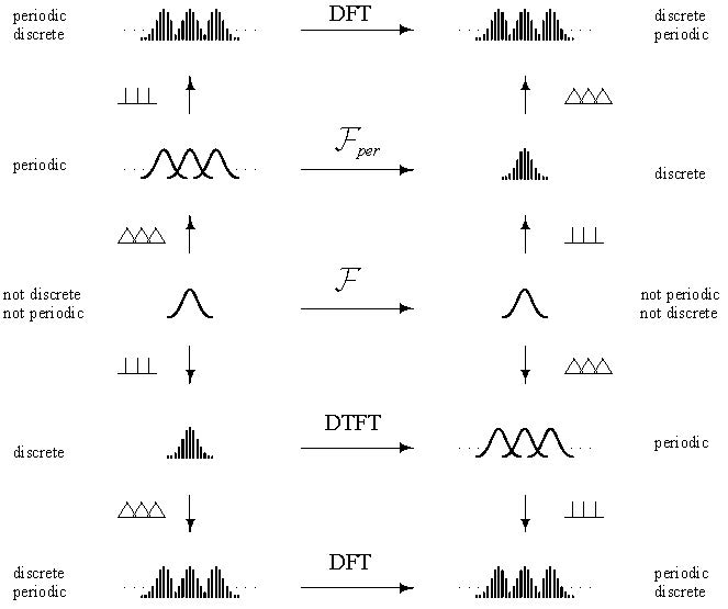
5. Four Fourier Transforms

The Poisson Summation Formula in its original version is commonly known to be true on Schwartz functions $f\in \mathcal{S}$, see e.g., [16]. The next theorem extends this understanding to a validity on tempered distributions including non-integrable functions $f\in {\mathcal{O}}_M$ and truly generalized functions $f\in {{\mathcal{O}}_C}^{\prime }$. Particular cases are the Dirac impulse $\delta \in {{\mathcal{O}}_C}^{\prime }$ in (28) and the function that is constantly $1\in {\mathcal{O}}_M$ in (29).

Theorem 1 (Four Fourier Transforms reduce to one Fourier Transform).

Let four Fourier transforms be defined as (A1), (A3), (A5) and (A7) and let us denote the integral Fourier transform (A1) as

$$\mathcal{F}(f)=\widehat{f}.$$

(27)

It then follows that the other three Fourier transform definitions (A3), (A5) and (A7) reduce to the known rules

$$\begin{array}{ccc}\hfill \mathcal{F}({▵▵▵}_T& f)\hfill & =\frac{1}{T}{\perp \perp \perp }_{\frac{1}{T}}\widehat{f}\hfill \end{array}$$

(28)

$$\begin{array}{ccc}\hfill \mathcal{F}({\perp \perp \perp }_{\frac{1}{T}}& f)\hfill & =T{▵▵▵}_T\widehat{f}\hfill \end{array}$$

(29)

$$\begin{array}{ccc}\hfill \mathcal{F}(\perp \perp \perp {▵▵▵}_N& f)\hfill & =\frac{1}{N}▵▵▵{\perp \perp \perp }_{\frac{1}{N}}\widehat{f}\hfill \end{array}$$

(30)

$$\begin{array}{ccc}\hfill \mathcal{F}(▵▵▵{\perp \perp \perp }_{\frac{1}{N}}& f)\hfill & =N\perp \perp \perp {▵▵▵}_N\widehat{f}\hfill \end{array}$$

(31)

where $\perp \perp \perp$ is discretization, $▵▵▵$ is periodization, defined as in (13) and (14), $T>0$ is real, $N>0$ an integer and

• (27) is the Integral Fourier Transform $\mathcal{F}$ (for non-discrete non-periodic functions) in ${\mathcal{S}}^{\prime }$,
• (28) is the Integral Fourier Transform ${\mathcal{F}}_{per}$ for (non-discrete) periodic functions in ${\mathcal{S}}^{\prime }$,
• (29) is its inverse, the DTFT for discrete (non-per.) functions in ${\mathcal{S}}^{\prime }$,
• (30) is the DFT for discrete periodic functions in ${\mathcal{S}}^{\prime }$,
• (31) is its inverse, the inverse Discrete Fourier Transform (IDFT) for discrete periodic functions in ${\mathcal{S}}^{\prime }$

and Equations (27)–(30) hold in the tempered distributions sense if

• $f\in {\mathcal{S}}^{\prime }=\mathcal{F}({\mathcal{S}}^{\prime })$ in (27),
• $f\in {{\mathcal{O}}_C}^{\prime }=\mathcal{F}({\mathcal{O}}_M)$ in (28),
• $f\in {\mathcal{O}}_M=\mathcal{F}({{\mathcal{O}}_C}^{\prime })$ in (29) and
• $f\in \mathcal{S}=\mathcal{F}(\mathcal{S})$ in (30) and (31).

Furthermore,

• (28) and (29) are dual generalizations of the Poisson Summation Formula (PSF) and
• (30) and (31) are (28) and (29) nested into one another in two different ways.

Finally, for any $f\in \mathcal{S}$, it follows that (27)–(31) hold simultaneously in ${\mathcal{S}}^{\prime }$.

Proof. 

The symbolic derivation of (28)–(31) from (A1), (A3), (A5) and (A7) is shown in Appendix B and their validities in ${\mathcal{S}}^{\prime }$ follow from Lemmas 1–8. The circumstance that (28) and (29) describe generalized variants of the PSF is shown in Section 2.4 and nesting them into one another yields (30) and (31) according to Lemmas 7 and 8. The last statement, finally, is already known [16]. □

Roughly, the theorem states that “instead of four Fourier transforms there is only one and instead of one PSF there are actually four”. Let us furthermore recall that requiring $f\in {\mathcal{O}}_M$ in (29), which means that it is infinitely differentiable and bounded by a polynomial, is not too strong for a function to be sampled.

Remark 1 (Bandlimitness).

In all practical cases, f is bandlimited in the sense that $\mathcal{F}f\in {{\mathcal{O}}_C}^{\prime }$ and this already fulfills the requirement $f\in {\mathcal{O}}_M$. Vice versa, if $f\notin {\mathcal{O}}_M$ then $\mathcal{F}f\notin {{\mathcal{O}}_C}^{\prime }$. Hence, f cannot be bandlimited. One may recall that the space of compactly supported tempered distributions ${\mathcal{E}}^{\prime }$ is a proper subspace of ${{\mathcal{O}}_C}^{\prime }$ (see above). The condition $\mathcal{F}f\in {{\mathcal{O}}_C}^{\prime }$ may therefore be understood as a wider comprehension of bandlimitness.

The interlinking formulas (28)–(31) can be visualized in a straightforward diagram (Figure 1). For simplicity, we use a Gaussian, i.e., a so-called self-reciprocal function [78], to withhold an existing reciprocity $t^{-1}\mapsto t^{+1}$ or $t^{+1}\mapsto t^{-1}$ between time (left or right column) and frequency (right or left column). More generally, wide Gaussians become narrow Gaussians and narrow Gaussians become wide Gaussians. One may notice that starting from the integral Fourier transform (middle row) at least Schwartz functions can reach the domain of the DFT (above and below). That is what we proved in Lemmas 7 and 8. It is also clear that “above” and “below” coincide. Hence, the diagram is double-cyclic (two cycles in opposite directions). Identifying the upper left side with the lower right side, we may also think of it as a Möbius band (only one cycle in either direction). It tells us that there is actually no left-hand side and no right-hand side, just opposite sides.

Figure 1. Four Fourier transforms and the links $\perp \perp \perp$ and $▵▵▵$ between them. In the tempered distributions sense, all four transforms $\mathcal{F},{\mathcal{F}}_{per},$ DTFT and DFT reduce to only one Fourier transform, the Fourier transform on tempered distributions.

6. Discussion

The PSF in its four variants is the actual link between the four usually defined Fourier transforms. The naming of these four Fourier transforms $\mathcal{F}$, ${\mathcal{F}}_{per}$, DTFT and DFT in the literature is often not very appropriate and sometimes confusing. They should be called “Fourier transform”, “Fourier transform for periodic functions”, “Fourier transform for discrete functions” and “Fourier transform for discrete periodic functions” more appropriately. All four transforms moreover describe special cases of the Fourier transform on tempered distributions; they only differ in the kind of functions to which they are applied, i.e., to $f,{▵▵▵}_{T}f,{\perp \perp \perp }_{\frac{1}{B}}f$ or ${▵▵▵}_T{\perp \perp \perp }_{\frac{1}{B}}f.$ An introduction of two transforms ${\mathcal{F}}_{per}$ and DTFT is generally not advisable because they are, apart from having an inverse sign (which indicates that they are inverse to one another), the same transform. Most appropriately, it could be called the “Fourier Series Transform” as it switches between two Fourier series representations, i.e., between discrete functions (Fourier series coefficients) and periodic functions (Fourier series). Its two formulas should be called “Fourier Series Analysis” and “Fourier Series Synthesis” formula, as already done in many textbooks.

Furthermore, it is shown that to be able to sample a function, it must be smooth and bounded by a polynomial. If one of these two properties is not given, the function is not bandlimited. Hence, the periodization of its Fourier transform will fail. These two conditions moreover represent a validity statement for variants of the PSF on tempered distributions.

Remark 2 (Sinc vs. Rect).

The Fourier transform pair $\{sinc$, $rect\}$ mentioned in the introduction above is a striking example for applying the validity statement for PSF variants as discussed in this study. The Equations (1) and (2) hold if $g\equiv sinc$ and $f\equiv rect$ but they fail if $f\equiv sinc$ and $g\equiv rect$ and the reason for this phenomenon is that

$$\begin{array}{ccc}\hfill rect& \in {{\mathcal{O}}_C}^{\prime }\hfill & \mathit{but}rect\notin {\mathcal{O}}_{M}and\hfill \\ \hfill sinc& \in {\mathcal{O}}_M\hfill & \mathit{but}sinc\notin {{\mathcal{O}}_C}^{\prime }\hfill \end{array}$$

which can easily be seen because $rect$ is of compact support and therewith it is rapidly decreasing ($\in {{\mathcal{O}}_C}^{\prime }$). However, it is not smooth in the ordinary functions sense ($\notin {\mathcal{O}}_M$). In contrast, $sinc$ is smooth in the ordinary functions sense ($\in {\mathcal{O}}_M$) but slowly decreasing ($\notin {{\mathcal{O}}_C}^{\prime }$), it goes with $1/t$ towards infinity which is a polynomial decrease. However, since $rect\in {{\mathcal{O}}_C}^{\prime }$ it can be periodized and since $sinc\in {\mathcal{O}}_M$, it can be discretized. A particular case arising from these facts is $▵▵▵(rect)=1$ and $\perp \perp \perp (sinc)=\delta$, respectively. Let us add them as Rule 19 and Rule 20 in Table 1.

Remark 3 (Shannon’s formula fails in $𝒮$′).

Another consequence of this slow decrease of $sinc$ is its failure to serve as a universal building block in Shannon’s [79] (and Kotelnikov’s [80]) reconstruction formula whenever we restore functions from samples. This reconstruction formula fails in ${\mathcal{S}}^{\prime }$ on arbitrary tempered distributions [3]. Equivalently, because $rect$ is no infinitely differentiable function, it cannot be used to cut out one period of arbitrary periodic tempered distributions. However, instead of the Fourier transform pair $\{sinc$, $rect\}$ there are other suitable building blocks (Lighthill’s unitary functions [22,81]) for reconstructing tempered distributions. We will treat them in a future paper in greater detail.

Appendix A.1. Conventional Fourier Transforms

Let $f(t)$ be a suitable function such that it can be Fourier transformed and let $\widehat{f}(\sigma )$ be its Fourier transform. Then the following four Fourier transform variants are usually defined.

Appendix A.1.1. Fourier Transform

The Integral Fourier Transform (for non-discrete non-periodic functions) is defined by

$$\begin{array}{ccc}\widehat{f}(\sigma )\hfill & ={\int }_{-\infty }^{\infty }f(t)e^{-2\pi it\sigma }dt\hfill & \mathrm{Analysis}\hfill \end{array}$$

(A1)

$$\begin{array}{ccc}f(t)\hfill & ={\int }_{-\infty }^{\infty }\widehat{f}(\sigma )e^{2\pi i\sigma t}d\sigma \hfill & \mathrm{Synthesis}\hfill \end{array}$$

(A2)

for suitable $f(t)$.

Appendix A.1.2. Fourier Transform (for Periodic Functions)

The Integral Fourier Transform for (non-discrete) periodic functions, used for Fourier Series analysis, is defined by

$$\begin{array}{ccccc}\widehat{f}[m]\hfill & =\frac{1}{T}\hfill & {\int }_0^T\hfill & f(t)e^{-2\pi i\frac{t}{T}m}dt\hfill & \mathrm{Analysis}\hfill \end{array}$$

(A3)

$$\begin{array}{ccccc}f(t)\hfill & =\hfill & \stackrel{\infty }{\sum _{m=-\infty }}\hfill & \widehat{f}[m]e^{2\pi i\frac{m}{T}t}\hfill & \mathrm{Synthesis}\hfill \end{array}$$

(A4)

where (A4) is the Fourier Series of $f(t)$ and (A3) determines its coefficients. The coefficients are discrete.

Appendix A.1.3. Fourier Transform (for Discrete Functions)

The Fourier Transform for discrete (non-periodic) functions, also called DTFT, used for Fourier Series synthesis, is defined by

$$\begin{array}{ccccc}\widehat{f}(\sigma )\hfill & =\frac{1}{T}\hfill & \stackrel{\infty }{\sum _{k=-\infty }}\hfill & f[k]e^{-2\pi i\frac{k}{T}\sigma }\hfill & \mathrm{Analysis}\hfill \end{array}$$

(A5)

$$\begin{array}{ccccc}f[k]\hfill & =\hfill & {\int }_0^T\hfill & \widehat{f}(\sigma )e^{2\pi i\frac{\sigma }{T}k}d\sigma \hfill & \mathrm{Synthesis}\hfill \end{array}$$

(A6)

where (A5) is a Fourier Series. Hence, it is periodic but $f(t)$ itself is discrete, its samples are determined by (A6).

Appendix A.1.4. Fourier Transform (for Discrete Periodic Functions)

The Fourier Transform for discrete periodic functions, called DFT is defined by

$$\begin{array}{cccc}\widehat{f}[m]\hfill & =\frac{1}{N}\hfill & \sum _{k=0}^{N-1}f[k]e^{-2\pi i\frac{k}{N}m}\hfill & \mathrm{Analysis}\hfill \end{array}$$

(38)

$$\begin{array}{cccc}f[k]\hfill & =\hfill & \sum _{m=0}^{N-1}\widehat{f}[m]e^{2\pi i\frac{m}{N}k}\hfill & \mathrm{Synthesis}\hfill \end{array}$$

(39)

where both (A7) and (A8) are (finite-sum) Fourier Series. Thus, they are periodic and discrete, simultaneously.

Appendix A.2. Distributional Fourier Transform

Let $⟨f,\phi ⟩$ be the application of a tempered distribution $f\in {\mathcal{S}}^{\prime }$ to some test function $\phi \in \mathcal{S}$. The Fourier transform of $f\in {\mathcal{S}}^{\prime }$ is then defined as

$$⟨\mathcal{F}f,\phi ⟩:=⟨f,\mathcal{F}\phi ⟩$$

where $\mathcal{F}$ on the right-hand side is the integral Fourier transform given by (A1) and its inverse is (A2), respectively. One usually uses this definition to test and verify symbolic calculation rules on tempered distributions. Once the rules are established, they can symbolically be used on tempered distributions as if they were ordinary functions. It is known that Fourier transform rules which apply to Lebesgue-square integrable functions do also apply to tempered distributions. Additionally, new rules can be found such as $\mathcal{F}1=\delta$ and $\mathcal{F}\delta =1$ which are based on rigorous calculations using the above definition. Rules summarized in Table 1 were established in [7]. They do also hold on ordinary square-integrable functions under the same conditions.

Most convenient is the fact that using the Fourier transform in the distributional sense, all functions become infinitely differentiable. In other words, the Fourier transform rule “multiplying a function k times with $2\pi it$ in one domain means to differentiate its Fourier transform k times in the other domain”, e.g., in [3,6,13,32,34,69], can be exploited unrestrictedly. One may recall that $2\pi it$ is the inner derivative of $e^{2\pi it\sigma }$. It means, the Fourier transform rule originates from

$$\frac{d}{d\sigma }{e}^{2\pi it\sigma }=(2\pi it)e^{2\pi it\sigma }$$

because $e^{2\pi it\sigma }$ is infinitely differentiable in the ordinary functions sense. The special role of $e^{2\pi it\sigma }$ arises from the fact that it is a number and a function, simultaneously.

Appendix B.1. Fourier Transform for Periodic Functions ($ℱ$_per)

In this subsection we will see that if a periodic function is Fourier transformed via the Fourier transform for periodic functions (A3) then the result is a discrete function. Indeed, inserting some $p(t)=({▵▵▵}_{T}f)(t)$ into (A3) yields

$$\begin{array}{ccc}\hfill \widehat{p}(m)& =\frac{1}{T}\hfill & {\int }_0^T{▵▵▵}_{T}f(t)e^{-2\pi i\frac{m}{T}t}dt\hfill \\ & =\frac{1}{T}\hfill & {\int }_{-\infty }^{\infty }f(t)e^{-2\pi i\frac{m}{T}t}dt\hfill \\ & =\frac{1}{T}\hfill & (\mathcal{F}f)(\frac{m}{T})\hfill \end{array}$$

where we used the popular periodization trick [17] and Fourier transform definition (A1). Inserting these coefficients into (A4) we obtain

$$\begin{array}{cc}\hfill ({▵▵▵}_{T}f)(t)& =\frac{1}{T}\stackrel{\infty }{\sum _{m=-\infty }}(\mathcal{F}f)(\frac{m}{T})e^{2\pi it\frac{m}{T}}\hfill \\ & =\frac{1}{T}{\mathcal{F}}^{-1}\left\{\stackrel{\infty }{\sum _{m=-\infty }}(\mathcal{F}f)(\frac{m}{T})\delta (\sigma -\frac{m}{T})\right\}\hfill \\ & =\frac{1}{T}{\mathcal{F}}^{-1}\left\{({\perp \perp \perp }_{\frac{1}{T}}(\mathcal{F}f))(\sigma )\right\}\hfill \\ & =\frac{1}{T}({\mathcal{F}}^{-1}{\perp \perp \perp }_{\frac{1}{T}}\mathcal{F}f)(t)\hfill \\ \hfill (\mathcal{F}({▵▵▵}_{T}f))(\sigma )& =\frac{1}{T}({\perp \perp \perp }_{\frac{1}{T}}(\mathcal{F}f))(\sigma ).\hfill \end{array}$$

Therefore, (A3) inserted into (A4) reduces to

$$\mathcal{F}({▵▵▵}_{T}f)=\frac{1}{T}{\perp \perp \perp }_{\frac{1}{T}}(\mathcal{F}f)$$

as a function of $\sigma \in \mathbb{R}$. This is formula (28).

Appendix B.2. Fourier Transform for Discrete Functions (DTFT)

We show that if a discrete function is Fourier transformed via the DTFT then the result is a periodic function. As (A5) is a Fourier series, it is periodic. The ansatz is therefore to let $\widehat{d}(\sigma )=({▵▵▵}_T\widehat{f})(\sigma )=({▵▵▵}_T(\mathcal{F}f))(\sigma )$ in (A6). It yields

$$\begin{array}{cc}\hfill d(k)& ={\int }_0^T{▵▵▵}_T\widehat{f}(\sigma )e^{2\pi i\frac{k}{T}\sigma }d\sigma \hfill \\ & ={\int }_{-\infty }^{\infty }\widehat{f}(\sigma )e^{2\pi i\frac{k}{T}\sigma }d\sigma \hfill \\ & =({\mathcal{F}}^{-1}(\mathcal{F}f))(\frac{k}{T})=f(\frac{k}{T}).\hfill \end{array}$$

Inserting these coefficients into (A5) we obtain

$$\begin{array}{cc}\hfill ({▵▵▵}_T(\mathcal{F}f))(\sigma )& =\frac{1}{T}\stackrel{\infty }{\sum _{k=-\infty }}f(\frac{k}{T})e^{-2\pi i\sigma \frac{k}{T}}\hfill \\ & =\frac{1}{T}\mathcal{F}\left\{\stackrel{\infty }{\sum _{k=-\infty }}f(\frac{k}{T})\delta (t-\frac{k}{T})\right\}\hfill \\ & =\frac{1}{T}\mathcal{F}\left\{({\perp \perp \perp }_{\frac{1}{T}}f)(t)\right\}\hfill \\ & =\frac{1}{T}(\mathcal{F}({\perp \perp \perp }_{\frac{1}{T}}f))(\sigma ).\hfill \end{array}$$

Thus, (A6) inserted into (A5) reduces to

$$\mathcal{F}({\perp \perp \perp }_{\frac{1}{T}}f)=T{▵▵▵}_T(\mathcal{F}f)$$

as a function of $\sigma \in \mathbb{R}$. This is formula (29).

Appendix B.3. Fourier Transform for Discrete Periodic Functions (DFT)

We show that if a discrete periodic function is Fourier transformed via the DFT, then the result is again a discrete periodic function. First, a simple reasoning tells us that after discretizing a periodic function $({▵▵▵}_{T}f)(t)$ it can be denoted as $y(t)=(\perp \perp \perp {▵▵▵}_{N}f)(t)$ where N is an integer corresponding to its period T. Inserting now its coefficients $({▵▵▵}_{N}f)(k)$ with $k\in \mathbb{Z}$ into (A7) yields

$$\begin{array}{cc}\hfill (\mathcal{F}({▵▵▵}_{N}f))(m)& =\frac{1}{N}\stackrel{N-1}{\sum _{k=0}}({▵▵▵}_{N}f)(k)e^{-2\pi i\frac{m}{N}k}\hfill \\ & =\frac{1}{N}\stackrel{\infty }{\sum _{k=-\infty }}f(k)e^{-2\pi i\frac{m}{N}k}\hfill \\ & =\frac{1}{N}(\mathcal{F}(\perp \perp \perp f))(\frac{m}{N})\hfill \\ & =\frac{1}{N}(▵▵▵(\mathcal{F}f))(\frac{m}{N})\hfill \end{array}$$

using, again, the periodization trick (applied to a discrete function this time), the definition of discretization $\perp \perp \perp$ and a previous result (Rule 4). Inserting these coefficients into (A8) we obtain

$$\begin{array}{ccc}\hfill ({▵▵▵}_{N}f)(k)& =\frac{1}{N}\sum _{m=0}^{N-1}▵▵▵\hfill & (\mathcal{F}f)(\frac{m}{N})e^{2\pi ik\frac{m}{N}}\hfill \\ & =\frac{1}{N}\stackrel{\infty }{\sum _{m=-\infty }}\hfill & (\mathcal{F}f)(\frac{m}{N})e^{2\pi ik\frac{m}{N}}\hfill \\ & =\frac{1}{N}({\mathcal{F}}^{-1}{\perp \perp \perp }_{\frac{1}{N}}\hfill & (\mathcal{F}f))(k).\hfill \end{array}$$

again, with the periodization trick, discretization $\perp \perp \perp$ and the definition of ${\mathcal{F}}^{-1}$ this time. Thus, (A7) inserted into (A8) reduces to

$$\begin{array}{cc}\hfill ({▵▵▵}_{N}f)(k)& =\frac{1}{N}({\mathcal{F}}^{-1}{\perp \perp \perp }_{\frac{1}{N}}(\mathcal{F}f))(k),k\in \mathbb{Z}\hfill \\ \hfill (\perp \perp \perp {▵▵▵}_{N}f)(t)& =\frac{1}{N}(\perp \perp \perp {\mathcal{F}}^{-1}{\perp \perp \perp }_{\frac{1}{N}}(\mathcal{F}f))(t),t\in \mathbb{R}\hfill \end{array}$$

and with Rule 3 applied backwards and Fourier transforming both sides it yields

$$\begin{array}{cc}\hfill \mathcal{F}(\perp \perp \perp {▵▵▵}_{N}f)& =\frac{1}{N}▵▵▵{\perp \perp \perp }_{\frac{1}{N}}(\mathcal{F}f)\hfill \end{array}$$

being a function of $\sigma \in \mathbb{R}$.

Appendix B.4. Derivation of the Inverse DFT

As (A7) is a Fourier series, it is periodic. Evaluating (A8) for $\widehat{g}(m)=({▵▵▵}_N\widehat{f})(m)$ where $\widehat{f}=\mathcal{F}f$ yields

$$\begin{array}{cc}\hfill g(k)& =\sum _{m=0}^{N-1}({▵▵▵}_N(\mathcal{F}f))(m)e^{2\pi i\frac{k}{N}m}\hfill \\ & =\stackrel{\infty }{\sum _{k=-\infty }}(\mathcal{F}f)(m)e^{2\pi i\frac{k}{N}m}\hfill \\ & =({\mathcal{F}}^{-1}\perp \perp \perp (\mathcal{F}f))(\frac{k}{N})\hfill \\ & =({\mathcal{F}}^{-1}\mathcal{F}(▵▵▵f))(\frac{k}{N})\hfill \\ & =(▵▵▵f)(\frac{k}{N})\hfill \end{array}$$

and inserting this result into (A7) we obtain

$$\begin{array}{cc}\hfill ({▵▵▵}_N(\mathcal{F}f))(m)& =\frac{1}{N}\stackrel{N-1}{\sum _{k=0}}(▵▵▵f)(\frac{k}{N})e^{-2\pi im\frac{k}{N}}\hfill \\ & =\frac{1}{N}\stackrel{\infty }{\sum _{k=-\infty }}f(\frac{k}{N})e^{-2\pi im\frac{k}{N}}\hfill \\ & =\frac{1}{N}(\mathcal{F}({\perp \perp \perp }_{\frac{1}{N}}f))(m).\hfill \end{array}$$

Thus, (A8) inserted into (A7) reduces to

$$\begin{array}{cc}\hfill (\mathcal{F}({\perp \perp \perp }_{\frac{1}{N}}f))(m)& =N({▵▵▵}_N(\mathcal{F}f))(m),m\in \mathbb{Z}\hfill \\ \hfill (\perp \perp \perp \mathcal{F}({\perp \perp \perp }_{\frac{1}{N}}f))(\sigma )& =N(\perp \perp \perp {▵▵▵}_N(\mathcal{F}f))(\sigma ),\sigma \in \mathbb{R}\hfill \end{array}$$

and with Rule 3 on the left-hand side (backwards) it yields

$$\begin{array}{cc}\hfill \mathcal{F}(▵▵▵{\perp \perp \perp }_{\frac{1}{N}}f)& =N\perp \perp \perp {▵▵▵}_N(\mathcal{F}f)\hfill \end{array}$$

being a function of $\sigma \in \mathbb{R}$.

Altogether, we proved that the DFT together with its inverse follow these two rules

$$\begin{array}{ccc}\hfill \mathcal{F}(\perp \perp \perp {▵▵▵}_{N}f)& =\frac{1}{N}\hfill & ▵▵▵{\perp \perp \perp }_{\frac{1}{N}}(\mathcal{F}f)\mathrm{and}\hfill \\ \hfill \frac{1}{N}\mathcal{F}(▵▵▵{\perp \perp \perp }_{\frac{1}{N}}f)& =\hfill & \perp \perp \perp {▵▵▵}_N(\mathcal{F}f)\hfill \end{array}$$

as functions of $\sigma \in \mathbb{R}$, which are (30) and (31), respectively.

References

- Zayed, A.I. Handbook of Function and Generalized Function Transformations; CRC Press Inc.: Boca Raton, FL, USA, 1996. [Google Scholar]
- Woodward, P.M. Probability and Information Theory, with Applications to Radar; Pergamon Press Ltd.: Oxford, UK, 1953. [Google Scholar]
- Gasquet, C.; Witomski, P. Fourier Analysis and Applications: Filtering, Numerical Computation, Wavelets; Springer: New York, NY, USA, 1999; Volume 30. [Google Scholar]
- Panaretos, A.H.; Anastassiu, H.T.; Kaklamani, D.I. A Note on the Poisson Summation Formula and Its Application to Electromagnetic Problems Involving Cylindrical Coordinates. Turk. J. Electr. Eng. Comput. Sci. 2002, 10, 377–384. [Google Scholar]
- Benedetto, J.J.; Zimmermann, G. Sampling Multipliers and the Poisson Summation Formula. J. Fourier Anal. Appl. 1997, 3, 505–523. [Google Scholar] [CrossRef]
- Strichartz, R.S. A Guide to Distribution Theorie and Fourier Transforms; World Scientific Publishing Co. Pte Ltd.: Singapore, 2003. [Google Scholar]
- Fischer, J. Anwendung der Theorie der Distributionen auf ein Problem in der Signalverarbeitung. Diploma Thesis, Ludwig-Maximillians-Universität München, Munich, Germany, 1997. [Google Scholar]
- Kiselman, C.O. Generalized Fourier transformations: The work of Bochner and Carleman viewed in the light of the theories of Schwartz and Sato. In Microlocal Analysis and Complex Fourier Analysis; World Scientific: Singapore, 2002; pp. 166–185. [Google Scholar]
- Taylor, M.E. Pseudodifferential Operators; Princeton University Press: Princeton, NJ, USA, 1981. [Google Scholar]
- Halperin, I.; Schwartz, L. Introduction to the Theory of Distributions; University of Toronto Press, Scholarly Publishing: Toronto, ON, Canada, 1952. [Google Scholar]
- Schwartz, L. Théorie des Distributions, Tome I; Hermann: Paris, France, 1950. [Google Scholar]
- Schwartz, L. Théorie des Distributions, Tome II; Hermann: Paris, France, 1951. [Google Scholar]
- Kammler, D.W. A First Course in Fourier Analysis; Cambridge University Press: Cambridge, UK, 2007. [Google Scholar]
- Benedetto, J.J. Harmonic Analysis and Applications; CRC Press Inc.: Boca Raton, FL, USA, 1996. [Google Scholar]
- Grafakos, L. Modern Fourier Analysis; Springer Science+Business Media: New York, NY, USA, 2009; Volume 250. [Google Scholar]
- Feichtinger, H.G.; Strohmer, T. Gabor Analysis and Algorithms: Theory and Applications; Birkhäuser: Boston, MA, USA, 1998. [Google Scholar]
- Gröchenig, K. Foundations of Time-Frequency Analysis; Birkhäuser: Basel, Switzerland, 2001. [Google Scholar]
- Brandwood, D. Fourier Transforms in Radar and Signal Processing; Artech House, Inc.: Norwood, MA, USA, 2003. [Google Scholar]
- Rahman, M. Applications of Fourier Transforms to Generalized Functions; WIT Press: Southampton, UK, 2011. [Google Scholar]
- Mallat, S.; Hwang, W.L. Singularity Detection and Processing with Wavelets. IEEE Trans. Inf. Theory 1992, 38, 617–643. [Google Scholar] [CrossRef]
- Temple, G. The Theory of Generalized Functions. Proc. R. Soc. Lond. Ser. A Math. Phys. Sci. 1955, 228, 175–190. [Google Scholar] [CrossRef]
- Lighthill, M.J. An Introduction to Fourier Analysis and Generalised Functions; Cambridge University Press: Cambridge, UK, 1958. [Google Scholar]
- Gelfand, I.M.; Schilow, G.E. Verallgemeinerte Funktionen (Distributionen), Teil I; VEB Deutscher Verlag der Wissenschaften: Berlin, Germany, 1960. [Google Scholar]
- Zemanian, A. Distribution Theory And Transform Analysis—An Introduction To Generalized Functions, with Applications; McGraw-Hill Inc.: New York, NY, USA, 1965. [Google Scholar]
- Trèves, F. Topological Vector Spaces, Distributions and Kernels: Pure and Applied Mathematics; Dover Publications Inc.: Mineola, NY, USA, 1967; Volume 25. [Google Scholar]
- Horváth, J. Topological Vector Spaces and Distributions; Addison-Wesley Publishing Company: Reading, MA, USA, 1966. [Google Scholar]
- Jones, D. The Theory of Generalized Functions; Cambridge University Press: Cambridge, UK, 1966. [Google Scholar]
- Zemanian, A.H. Generalized Integral Transformations; Dover Publications Inc.: Mineola, NY, USA, 1968. [Google Scholar]
- Gelfand, I.M.; Schilow, G.E. Verallgemeinerte Funktionen (Distributionen), Teil II, Zweite Auflage; VEB Deutscher Verlag der Wissenschaften: Berlin, Germany, 1969. [Google Scholar]
- Barros-Neto, J. An Introduction to the Theory of Distributions; Marcel Dekker Inc.: New York, NY, USA, 1973. [Google Scholar]
- Wagner, P. Zur Faltung von Distributionen. Math. Annalen 1987, 276, 467–485. [Google Scholar] [CrossRef]
- Hörmander, L. The Analysis of Linear Partial Differential Operators I, Die Grundlehren der mathematischen Wissenschaften; Springer: Berlin/Heidelberg, Germany, 1983. [Google Scholar]
- Walter, W. Einführung in die Theorie der Distributionen; BI-Wissenschaftsverlag, Bibliographisches Institut & FA Brockhaus: Mannheim, Germany, 1994. [Google Scholar]
- Vladimirov, V. Methods of the Theory of Generalized Functions; CRC Press Inc.: Boca Raton, FL, USA, 2002. [Google Scholar]
- Fischer, J.V. On the Duality of Discrete and Periodic Functions. Mathematics 2015, 3, 299–318. [Google Scholar] [CrossRef]
- Fischer, J.V. On the Duality of Regular and Local Functions. Mathematics 2017, 5, 41. [Google Scholar] [CrossRef]
- Reed, M.; Simon, B. II: Fourier Analysis, Self-Adjointness; Academic Press Inc.: New York, NY, USA, 1975; Volume II. [Google Scholar]
- Constantinescu, F. Distributions and Their Applications in Physics: International Series in Natural Philosophy; Pergamon Press Ltd.: Oxford, UK, 1980. [Google Scholar]
- Glimm, J.; Jaffe, A. Quantum Physics: A Functional Integral Point of View; Springer: New York, NY, USA, 1981. [Google Scholar]
- Folland, G.B. Harmonic Analysis in Phase Space; Princeton University Press: Princeton, NJ, USA, 1989. [Google Scholar]
- Saichev, A.I.; Woyczynski, W.A. Distributions in the Physical and Engineering Sciences. Volume 2—Linear and Nonlinear Dynamics of Continuous Media; Birkhäuser-Boston: Boston, MA, USA, 2013. [Google Scholar]
- Messiah, A. Quantum Mechanics—Two Volumes Bound as One; Dover Publications, Inc.: Mineola, NY, USA, 2003. [Google Scholar]
- Debnath, L. A Short Biography of Paul A M Dirac and Historical Development of Dirac Delta Function. Int. J. Math. Educ. Sci. Technol. 2013, 44, 1201–1223. [Google Scholar] [CrossRef]
- Dirac, P. The Principles of Quantum Mechanics; Oxford University Press: Oxford, UK, 1930. [Google Scholar]
- Dierolf, P. The Structure Theorem for Linear Transfer Systems. Note di Matematica 1991, 11, 119–125. [Google Scholar]
- Smith, D.C. An Introduction to Distribution Theory for Signals Analysis. Digit. Signal Process. 2006, 16, 419–444. [Google Scholar] [CrossRef]
- Osgood, B. The Fourier transform and its applications. In Lecture Notes for EE 261; Electrical Engineering Department, Stanford University: Stanford, CA, USA, 2007. [Google Scholar]
- Boche, H.; Mönich, U.J. Distributional Behavior of Convolution Sum System Representations. IEEE Trans. Sign. Proc. 2018, 66, 5056–5065. [Google Scholar] [CrossRef]
- Unser, M. Sampling—50 Years after Shannon. Proc. IEEE 2000, 88, 569–587. [Google Scholar] [CrossRef]
- Grossmann, A.; Loupias, G.; Stein, E.M. An Algebra of Pseudodifferential Operators and Quantum Mechanics in Phase Space. Ann. Inst. Fourier 1968, 18, 343–368. [Google Scholar] [CrossRef]
- Ashino, R.; Boggiatto, P.; Wong, M.W. Advances in Pseudo-Differential Operators; Birkhäuser Verlag: Basel, Switzerland, 2012; Volume 155. [Google Scholar]
- Feichtinger, H.G. Modulation Spaces on Locally Compact Abelian Groups; Universität Wien, Mathematisches Institut: Vienna, Austria, 1983. [Google Scholar]
- Gröchenig, K.; Heil, C. Modulation Spaces and Pseudodifferential Operators. Integr. Equ. Oper. Theory 1999, 34, 439–457. [Google Scholar] [CrossRef]
- Bényi, Á.; Gröchenig, K.; Okoudjou, K.A.; Rogers, L.G. Unimodular Fourier Multipliers for Modulation Spaces. J. Funct. Anal. 2007, 246, 366–384. [Google Scholar] [CrossRef]
- Feichtinger, H.G. On a New Segal Algebra. Monatsh. Math. 1981, 92, 269–289. [Google Scholar] [CrossRef]
- Özçağ, E. Defining the k-th Powers of the Dirac-Delta Distribution for Negative Integers. Appl. Math. Lett. 2001, 14, 419–423. [Google Scholar] [CrossRef]
- Li, C. The Powers of the Dirac Delta Function by Caputo Fractional Derivatives. J. Fract. Calc. Appl. 2016, 7, 12–23. [Google Scholar]
- Bracewell, R.N. Fourier Transform and its Applications; McGraw-Hill Book Company: New York, NY, USA, 1986. [Google Scholar]
- Dierolf, P. Multiplication and Convolution Operators between Spaces of Distributions. North-Holland Math. Stud. 1984, 90, 305–330. [Google Scholar]
- Gracia-Bondía, J.M.; Varilly, J.C. Algebras of Distributions Suitable for Phase-Space Quantum Mechanics. I. J. Math. Phys. 1988, 29, 869–879. [Google Scholar] [CrossRef]
- Dubois-Violette, M.; Kriegl, A.; Maeda, Y.; Michor, P.W. Smooth*-Algebras. arXiv, 2001; arXiv:math/0106150. [Google Scholar]
- Ortner, N. On Convolvability Conditions for Distributions. Monatsh. Math. 2010, 160, 313–335. [Google Scholar] [CrossRef]
- Larcher, J. Multiplications and Convolutions in L. Schwartz’ Spaces of Test Functions and Distributions and their Continuity. Analysis 2013, 33, 319–332. [Google Scholar] [CrossRef]
- Ortner, N.; Wagner, P. On the Spaces of John Horváth. J. Math. Anal. Appl. 2014, 415, 62–74. [Google Scholar] [CrossRef]
- Katznelson, Y. Une remarque concernant la formule de Poisson. Stud. Math. 1967, 29, 107–108. [Google Scholar] [CrossRef]
- Butzer, P.L.; Stens, R. The Poisson Summation Formula, Whittaker’s Cardinal Series and Approximate Integration. In Second Edmonton Conference on Approximation Theory; American Mathematical Society: Providence, RI, USA, 1983; pp. 19–36. [Google Scholar]
- Kahane, J.P.; Lemarié-Rieusset, P.G. Remarques sur la formule sommatoire de Poisson. Stud. Math. 1994, 109, 303–316. [Google Scholar] [CrossRef]
- Gröchenig, K. An Uncertainty Principle related to the Poisson Summation Formula. Stud. Math. 1996, 121, 87–104. [Google Scholar] [CrossRef]
- Nguyen, H.Q.; Unser, M.; Ward, J.P. Generalized Poisson Summation Formulas for Continuous Functions of Polynomial Growth. J. Fourier Anal. Appl. 2017, 23, 442–461. [Google Scholar] [CrossRef]
- Lyness, J. The Calculation of Fourier Coefficients by the Möbius Inversion of the Poisson Summation Formula. I. Functions whose early derivatives are continuous. Math. Comput. 1970, 24, 101–135. [Google Scholar]
- Kerl, J. Poisson Summation and the Discrete Fourier Transform. 2008. Available online: https://johnkerl.org/doc/fourpoi.pdf (accessed on 8 October 2018).
- Cumming, I.G.; Wong, F.H. Digital Processing of Synthetic Aperture Radar Data; Artech House: Norwood, MA, USA, 2005. [Google Scholar]
- Feichtinger, H.G. Thoughts on Numerical and Conceptual Harmonic Analysis. In New Trends in Applied Harmonic Analysis; Birkhäuser: Cham, Switzerland, 2016; pp. 301–329. [Google Scholar]
- Susskind, L.; Friedman, A. Quantum Mechanics: The Theoretical Minimum; Pinguin Random House: Alan Lane, UK, 2014. [Google Scholar]
- Baggott, J. The Meaning of Quantum Theory: A Guide for Students of Chemistry and Physics; Oxford University Press: New York, NY, USA, 1992. [Google Scholar]
- Arici, F.; Becker, D.; Ripken, C.; Saueressig, F.; van Suijlekom, W.D. Reflection Positivity in Higher Derivative Scalar Theories. J. Math. Phys. 2018, 59, 082302. [Google Scholar] [CrossRef]
- Paule, P.; Schneider, C. Towards a Symbolic Summation Theory for Unspecified Sequences. arXiv, 2018; arXiv:1809.06578. [Google Scholar]
- Born, M. Reciprocity Theory of Elementary Particles. Rev. Mod. Phys. 1949, 21, 463. [Google Scholar] [CrossRef]
- Shannon, C.E. Communication in the Presence of Noise. Proc. IRE 1949, 37, 10–21. [Google Scholar] [CrossRef]
- Schirman, J.D. Theoretische Grundlagen der Funkortung; Militärverlag der DDR: Berlin, Germany, 1977. [Google Scholar]
- Boyd, J.P. Construction of Lighthill’s Unitary Functions: The Imbricate Series of Unity. Appl. Math. Comput. 1997, 86, 1–10. [Google Scholar] [CrossRef]
© 2018 by the author. Licensee MDPI, Basel, Switzerland. This article is an open access article distributed under the terms and conditions of the Creative Commons Attribution (CC BY) license (http://creativecommons.org/licenses/by/4.0/).