A Model and an Algorithm for a Large-Scale Sustainable Supplier Selection and Order Allocation Problem

Abstract

We consider a buyer’s decision problem of sustainable supplier selection and order allocation (SSS & OA) among multiple heterogeneous suppliers who sell multiple types of items. The buyer periodically orders items from chosen suppliers to refill inventory to preset levels. Each supplier is differentiated from others by the types of items supplied, selling price, and order-related costs, such as transportation cost. Each supplier also has a preset requirement for minimum order quantity or minimum purchase amount. In the beginning of each period, the buyer constructs an SSS & OA plan considering various information from both parties. The buyer’s planning problem is formulated as a mathematical model, and an efficient algorithm to solve larger instances of the problem is developed. The algorithm is designed to take advantage of the branch-and-bound method, and the special structure of the model. We perform computer experiments to test the accuracy of the proposed algorithm. The test result confirmed that the algorithm can find a near-optimal solution with only 0.82 percent deviation on average. We also observed that the use of the algorithm can increase solvable problem size by about 2.4 times.

1. Introduction

Supplier evaluation and selection are important decisions in the management of a supply network [1,2]. After determining suppliers to fill orders, the subsequent decision to allocate orders to chosen suppliers follows. Recent awareness in sustainable supply chain management frequently integrates these decisions with sustainability factors. The concept of sustainability plays an essential role in many organization and industries with respect to environmental protection and social responsibility [3]. As a consequence, sustainable supplier selection and order allocation (SSS & OA) emerges as a hot issue in the area of production and logistics. Huge number of papers have been published for this important decision problem. For example, Kuo et al. [4] developed a supplier selection system through fuzzy AHP and DEA. Their method was successfully applied to an auto lighting system company in Taiwan. The SSS & OA can be included in green supply chain management to improve the performance of a supply chain. Roehrich et al. [5] did such a study for a globalized German-based aircraft interior manufacturer and six key suppliers. There are a few commercial systems having supplier selection and evaluation functions. eSourcing Capability Models developed by ITSqc and CMMI-ACQ, made by SEI, are useful systems in the business area for acquiring products and services [6,7].

This paper studies an SSS & OA problem for a buyer who performs regular replenishment activities with heterogeneous suppliers who sell a few types of items. The system analyzed here is a two-stage supply chain system, which consists of a single buyer controlling inventories using a periodic order-up-to inventory control policy, and multiple heterogeneous suppliers who can supply items in response to orders from the buyer. The buyer sells items to end customers and replenishes items regularly based on the inventory status and future demand forecasts. In response to an order from the buyer, the suppliers transport the ordered amount after a constant lead time.

The problem analyzed in this paper is a buyer’s decision problem of selecting suppliers and, at the same time, order allocation for selected suppliers. Based on such replenishment decisions, the buyer considers various system variables and several contract terms, including minimum order quantity (MOQ) and minimum purchase amount (MPA) requirements. The MOQ and MPA specify that suppliers accept only those orders that exceed a predetermined minimum order quantity and minimum order value [8,9,10]. Additional factors the buyer considers in the decision process include working capital requirement and sustainability factors.

Even though several optimization model variants have been introduced for systems similar to the one analyzed in this paper, a detailed model representing all the important characteristics of the SSS & OA process has not yet been analyzed. To handle larger instances of real decision processes requiring big data and excessive computational capacity, an efficient new solution methodology is also desired to make full use of a developed model. Considering this research need, the current paper introduces a mathematical model and solution methodology, which are constructed by relaxation and ideas from the branch-and-bound method.

2. Literature Review

A large number of studies dealing with the supplier selection problem have been published. A recent survey paper reviewed 370 works in this area [11]. As stated in their review, the subjects of supplier selection problems are very wide, ranging from criteria analysis for supplier selection to multiple criteria inventory control problems. Among numerous topics studied in this area, our review of previous research is narrowly focused on the supplier selection and order allocation problem of a single buyer dealing with multiple items, as well as multiple suppliers requiring MOQ and MPA constraints, working capital requirement constraint, and sustainability features. Thus, the basic forms of research related to this paper can be classified into two sub-areas. The first sub-area is about supplier selection and order allocation, while the second area is the sustainable supplier selection and order allocation. Previous research on the two sub-areas are presented followed by a discussion on the research gaps and contribution of this paper.

2.1. Supplier Selection and Order Allocation

To solve the supplier selection and order allocation problem, Ghorbani et al. [12] proposed a two-phased model. At first, suppliers are evaluated according to both quantitative and qualitative criteria resulting from SWOT analysis. Shannon entropy is used to calculate criteria weights. Then, the results are used as an input for an integer linear programming model to allocate orders to suppliers. Nazari-Shirkouhi et al. [13] provided an integrated linear programming model that aimed to minimize total ordering costs and defective items. Jadidi et al. [14], [15] modeled the supplier selection as a multi-objective optimization model where minimization of price, rejects, and lead-time were considered as three objectives. Sodenkamp et al. [16] proposed a novel meta-approach for collaborative multi-objective supplier selection and order allocation (SSOA)decisions by combining multi-criteria decision analysis and linear programming. The proposed model accounted for suppliers’ performance synergy effects within a hierarchical decision-making process. Shabanpour et al. [17] proposed efficiency improvement plans for supplier selection, including goal programming and data envelopment analysis applications to rank sustainable suppliers.

In addition to usual constraints included in the previous research on SSOA, our model includes two other kinds of features practiced in the real world. The first constraint is MOQ/MPA-related practices, and the second is limitation caused by working capital management. Research concerning an SSOA considering the MOQ/MPA requirements was initiated by Robb and Silver [18]. Afterward, several researchers, including Kiesmüller et al. [9], Zhao and Katehakis [19], Zhou et al. [20], and Meena and Sarmah [21] have studied several variants of the SSOA problems with associated requirements. All of these studies could be categorized a basic model, because all studied a single-item problem. More realistic multi-item problems were first analyzed by Zhou [22], and Aktin and Gergin [23]. Recently, Park et al. [10] considered an order allocation problem with the MOQ/MPA requirements and proposed a rolling-horizon implementation strategy for solving a formulated optimization model more efficiently. Their model, however, did not contain a sustainability feature or working capital requirements.

Supply chain models typically only consider the physical transformation activities and disregard the financial implications of those activities. Recently, however, the literature on supply chain management (SCM) became aware of the real-world situation that financing and operational problems are closely connected and, thus, optimizing the two problems jointly could improve the entire performance of a supply chain [24,25]. However, only a few related papers were found on an SSOA with a working capital requirement (WCR). Chao et al. [26] developed recursive equations for a replenishment (order size determination) problem with a cash flow constraint. The problem was for a single item without considering supplier’s perspectives, and thus could be categorized as the primitive type of research compared with our current problem. Bendavid et al. [27] studied a buyer’s replenishment problem with a single type of item using a more sophisticated flow balance equation for the working capital constraint. Bian et al. [24] presented a new generic working capital requirement model for a single-item lot sizing problem. They presented a mixed integer programming model, including a flow balance equation, for operating working capital requirement (OWCR). To the best of our knowledge, there is no prior work addressing the SSOA problem that also directly considered WCR or OWCR.

2.2. Sustainable Supplier Selection and Order Allocation

The traditional supplier selection and order allocation problem has now been changed to an SSS & OA, where sustainability triple bottom line (3BL) attributes (environmental, economic, and social) are integrated into the selection and allocation processes [28]. The environmental factors can also be evaluated in terms of political, economic, social, technological, and environmental aspects, as can be seen in the well-known method named PESTEL [29]. The literature on sustainable supplier selection is quite rich. A few prior studies include [30,31,32,33,34,35,36,37,38,39,40,41,42,43,44,45,46,47,48]. These studies used various kinds of methods, including the AHP, DEMATEL, ANP, TOPSIS, multi-objective GA, DEA, and VIKOR for evaluating and selecting desirable sustainable suppliers. All the above referenced research deals with the question of which sustainable supplier to select. Research dealing with order allocation together with sustainable supplier selection is in its early stages. Only five papers on SSS & OA have been noted during the literature review. Kannan et al. [49] introduced a fuzzy TOPSIS method for supplier selection and a bi-objective model for order allocation. Govindan et al. [50] analyzed a five-echelon supply chain for assigning suppliers for a single product. Aktin and Gergin [23] introduced a mixed integer programming model using 3BL index scores. Problems analyzed in these three papers can be categorized as basic SSS & OA because they considered a single product and single period case with a deterministic demand. Recently, more sophisticated models have been offered by Gören [51] and Ghadimi et al. [1]. The former solved a problem with multiple products and suppliers, and formulated a bi-objective optimization model for a single period decision. The latter analyzed a similar system, but formulated it as a multi-period bi-objective model. However, both of these studies assumed a deterministic demand and did not consider other realistic features, such as transportation lead time or MOQ requirement.

2.3. Research Gap and the Contribution of This Paper

As can be found in the discussion of previous research and also in

Table 1. Comparison of the contributions of different authors.

Author(s)	Problem Type		Model Type		Demand Process			Number of Items		Number of Periods		New Solution Method	Constraints			Transportation Lead Time
	Supplier Selection	Order Allocation			Determi-nistic	Stochastic		Single Item	Multi-Item	Single Period	Multi-Period
			Single Supplier	Multiple Supplier		Stationary	Non-Stationa-ry						MOQ/MPA	WCM	Sustainability
Zhao and Katehakis [19]		√	√			√					√
Zhou et al. [20]		√	√			√		√			√
Chao et al. [26]		√	√			√		√			√	√		√
Zhou [22]		√	√			√			√		√		√
Kiesmüller et al. [9]		√	√			√		√			√		√			√
Kannan et al. [49]	√	√		√	√			√		√					√
Meena and Sarmah [21]	√	√		√	√			√		√			√
Govindan et al. [38]	√	√		√		√		√		√		√			√
Ayhan and Kilic [52]	√	√		√	√				√	√					√
Trapp and Sarkis [43]	√			√					√	√		√
Aktin and Gergin [23]	√	√		√	√				√	√					√
Bendavid et al. [27]		√	√			√		√			√			√
Gören [51]	√	√		√	√				√		√				√
Ghadimi et al. [1]	√	√		√	√				√	√					√
Bian et al. [24]		√	√		√			√			√	√		√
Park et al. [10]	√	√		√		√	√		√		√		√			√
This model	√	√		√		√	√		√		√	√	√	√	√	√

, our study is the first attempt to analyze the most realistic and complicated SSS & OA problem representing various important features of a real system, including transportation features (transportation lead times and capacity of the suppliers) and buyer monetary limitations (multi-period working capital flow balances and limitation, time value of money). Given the various aspects we are considering for this analysis, the optimization model introduced in this paper is the most sophisticated of any existing models representing SSS & OA activities. One of the challenges we experienced during the development of such a large-scale model is that none of the existing methods can solve our model to a desired accuracy within a practical time limit. For example, a problem with 20 items and 12 time periods cannot be solved within 24 h time limit. When we consider that real-world problems can include more than 100 items, it is necessary to fill this research gap. In response to this research challenge, a new algorithm specifically aimed to solve such a big model is developed. During a computational experiment, the algorithm is capable of solving such a model within a reasonable computational time with desired accuracy.

3. System Description and Assumptions

The system analyzed in this paper involves two or more heterogeneous suppliers and a single buyer. The suppliers are distinguished from each other by the type and selling prices of the items they carry, delivery lead times, and minimum order quantity requirements. The buyer carries multiple types of items which are sold to end customers. The items are replenished to minimize related inventory costs based on a periodic order-up-to inventory control policy. Previous research on inventory control frequently assumed that the end customer demand can be described by a known probability distribution. However, since the future demand for a product can be influenced by unforeseeable events, complete information on future demand distribution may not be available [53]. Considering this kind of real-world situation, this paper assumes that the demand of the end customers may not belong to a theoretical probability distribution. Other assumptions are as follows:

• There is a planned allocation schedule of money for each period during a planning horizon.
• Money remaining at the end of a period is inflated by interest rate and carried forward to the next period.
• Payment for purchase and transportation costs are made as an order is placed.
• Nonzero transportation lead time exists between an order placement and the arrival of the ordered amount.
• Major and minor ordering costs occur when an order is placed.
• The major ordering cost occurs as a fixed amount when an order is placed.
• The minor ordering cost occurs in proportion to an order size.
• A supplier has limited production capacity and thus has an order size limit per order.
• A supplier has a limited number of transportation vehicles.
• Any amount of an item can be purchased at a price higher than supplier’s regular price from a spot market.
• 3BL factor scores of each potential supplier are prepared for input to an SSS & OA decision.

Considering the characteristics of each supplier, the buyer must make an SSS & OA decision at the beginning of each period. The objective that the buyer is trying to achieve is to minimize the net present value of the related costs occurring throughout the planning horizon. Required notations are as follows.

Indices:

$i$	item number, $i=1,2,\cdots ,I,$
$j$	3BL index, $j=\mathrm{env},\mathrm{eco},\mathrm{soc},$
$k$	supplier number, $k=1,2,\cdots ,K,$
$t$	period, $t=1,2,\cdots ,T$, where $T$ denotes the end period of the planning horizon.

Parameters:

$K(i)$	set of suppliers who sell item $i$, $\forall i,$
$I(k)$	set of items sold by supplier $k$, $\forall k,$
$d_{it}$	demand forecast of item $i$ during future period $t$, $\forall i,t,$
${\xi }_{it}$	standard deviation of error of $d_{i,t}$, $\forall i,t,$
$v_i$	volume of item $i$, $\forall i,$
$w{c}_t$	warehouse capacity of the buyer during period $t$, $\forall t,$
$h_i$	holding cost of item $i$, $\forall i,$
$b_i$	shortage cost of item $i$, $\forall i,$
$p_{ikt}$	unit purchase price for item $i$ paid by the buyer to supplier $k$ during period $t$, $\forall i,k\in K(i),t,$
$p_{it}^s$	unit spot market price during period $t$ for item $i$, $\forall i,t,$
$owc{l}_t$	operating working capital limit in period t, $\forall t$,
$cap{t}_t$	capital originally allocated to period t, $\forall t$,
$i{c}_t$	inventory control related cost (holding plus shortage costs) in period t, $\forall t,$
$r{c}_t$	replenishment related cost in period t, $\forall t,$
$r$	per-period discount (interest) rate.
$mo{q}_{ik}$	per-period minimum order quantity specified by supplier $k$ for item $i$, $\forall i,k,$
$mp{a}_k$	per-period minimum purchase amount set by supplier $k$,$\forall k,$
$mp{l}_{ik}$	per-period maximum purchase limit for item $i$ specified by supplier $k,\forall i,k\in K(i),$
$m{a}_k$	major ordering cost for supplier $k$, $\forall k,$
$m{i}_{ik}$	minor ordering cost for item $i$ for supplier $k$, $\forall i,k\in K(i),$
$s{c}_{jk}$	$j$th 3BL factor score of supplier $k$, $\forall j,k,$
$targe{t}_{jt}$	$j$th 3BL factor target score of period $t$, $\forall j,t,$
$l_k$	supplier $k’\mathrm{s}$ lead time, $\forall k,$
$f_{kt}$	freight fair per vehicle of supplier $k$ during period $t$, $\forall t,k$,
$v{c}_k$	volume capacity per vehicle of supplier $k$, $\forall k,$
$n{v}_{kt}$	number of vehicles available for transportation of supplier $k$ in period $t$, $\forall k,$
${\tilde{x}}_{ikt}$	purchase already made at the start of past period $t$ and in delivery of item $i$ from supplier $k$, $\forall i,k\in K(i),t=-1,-2,\cdots ,1-l_k,$
$I{P}_{i0}$	inventory position of item $i$ at the start of planning, $\forall i,$
$M$	very large number.

Decision variables:

$I{P}_{it}$	inventory position of item $i$ at the end of period $t$, $\forall i,t,$
$I{P}_{it}^{+}$	positive part of $I{P}_{i,t}$, $\forall i,t,$
$I{P}_{it}^{-}$	negative part of $I{P}_{i,t}$, $\forall i,t,$
$x_{ik1}$	purchase amount of item $i$ from supplier $k$ during the present period (period 1), $\forall i,k\in K(i),$
$x_{ikt}$	planned purchase amount of item $i$ from supplier $k$ during future period $t$, $\forall i,k\in K(i),t=2,\cdots ,T,$
$x_{i1}^s$	purchase quantity of item $i$ from the spot market for the present period, $\forall i,$
$x_{it}^s$	planned purchase quantity of item $i$ from the spot market for period $t$, $\forall i,t=2,\cdots ,T,$
$R{L}_{it}$	replenishment level of item $i$ after the arrival of orders scheduled to arrive at the start of period $t$, $\forall i,t,$
$o_{jt}$	positive deviation from target ${}_{jt}$ in period $t$,
${\alpha }_{ikt}^{moq}$	binary integer for controlling the minimum order quantity requirement, $\forall i,k,t,$
${\alpha }_{kt}^{mpa}$	binary integer for controlling the minimum purchase amount requirement, $\forall k,t,$
${\beta }_{kt}^{MA}$	binary integer for controlling major ordering cost, $\forall k,t,$
${\beta }_{ikt}^{MI}$	binary integer for controlling minor ordering cost, $\forall i,k,t,$
${\theta }_i$	safety factor of item $i$, $\forall i$.

4. Model Formulation

4.1. Relevant Costs

Cost factors included in the total cost of our model are inventory-related costs (holding and shortage costs) and replenishment-related costs (major and minor ordering costs, transportation, and purchase costs). Inventory-related costs are the sum of inventory holding and shortage costs incurred during the planning horizon, and are expressed as in Equation (1).

$$i{c}_t={\displaystyle {\displaystyle \sum }_{i=1}^I}\left(\frac{1}{2}{h}_i(R{L}_{it}+I{P}_{it}^{+})+b_{i}I{P}_{it}^{-}\right),\forall t.$$

(1)

Transportation cost of period $t$ is

$${\displaystyle {\displaystyle \sum }_{k=1}^K}{f}_{kt}N{V}_{kt}.$$

Purchase cost is the sum of the payment to suppliers and spot market.

$${\displaystyle {\displaystyle \sum }_{i=1}^I}{\displaystyle {\displaystyle \sum }_{k\in K(i)}}{p}_{ikt}{x}_{ikt}+{\displaystyle {\displaystyle \sum }_{i=1}^I}s{p}_{it}{x}_{it}^s.$$

Major and minor ordering costs are as follows:

$${\displaystyle {\displaystyle \sum }_{k=1}^K}m{a}_k{\beta }_{kt}^{MA}+{\displaystyle {\displaystyle \sum }_{i=1}^I}{\displaystyle {\displaystyle \sum }_{k\in K(i)}}m{i}_{ik}{\beta }_{ikt}^{MI}.$$

Replenishment-related cost is the sum of the cost factors in Equation (2).

$$\begin{gathered} r{c}_t={\displaystyle {\displaystyle \sum }_{k=1}^K}(m{a}_k{\beta }_{kt}^{MA}+f_{kt}n{v}_{kt})+{\displaystyle {\displaystyle \sum }_{i=1}^I}{\displaystyle {\displaystyle \sum }_{k\in K(i)}}(p_{ikt}{x}_{ikt}+m{i}_{ik}{\beta }_{ikt}^{MI}) \\ +{\displaystyle {\displaystyle \sum }_{i=1}^I}s{p}_{it}{x}_{it}^s,\forall t. \end{gathered}$$

(2)

The total cost function of the model (TC) is the present value of inventory control cost plus replenishment-related cost incurred during the planning horizon. When we use a discounting factor $r$ to account for the time value of money, the cost function can be written as

$$TC={\displaystyle {\displaystyle \sum }_{t=1}^T}\frac{1}{{(1+r)}^t}(i{c}_t+r{c}_t).$$

4.2. Operating Working Capital Requirement

In practice, many firms are financially constrained; therefore, their ability to manage their inventories is directly affected by many factors, including their operating working capitals. To represent this financial constraint, the following equations are included.

$$i{c}_t+r{c}_t\le owc{l}_t,\forall t,$$

(3)

$$owc{l}_t=cap{t}_t+(1+\gamma )(owc{l}_{t-1}-r{c}_{t-1}-i{c}_{t-1}),\forall t.$$

(4)

Equation (3) specifies that the cost occurring during period t is limited by an operating working capital limit (OWCL) in that period. The equation was based on the cash-to-cash methodology found in Theodore Farris and Hutchison [54], and Hofmann and Kotzab [55]. Consequently, we assumed that the OWCR for replenishing a unit of product depends on the money invested in the related operations, for example, purchasing, setup, transportation, inventory holding, and shortage costs. Also, as in Bian et al. [24], it is assumed that the profit portion of the sales revenue is not accounted for in the OWCR. Profit can be allocated to other higher priority objectives of the firm (e.g., debt reduction, dividend payments, or internal and external investment). Thus, the profit portion of a firm’s activities was not represented in our model (e.g., Equations (3) and (4)). Equation (4) models monetary flow during two adjacent periods and ensures that the OWCL in period t equals the sum of the operating working capital (OCM) allocated to period t and the money left in the previous period inflated by interest and forwarded to the current period.

4.3. 3BL Target Constraints

$${\displaystyle {\displaystyle \sum }_{i=1}^I}{\displaystyle {\displaystyle \sum }_{k=1}^K}s{c}_{jk}{\beta }_{ikt}^{MI}-o_{jt}=targe{t}_{jt},\forall j,t.$$

(5)

As stated in Aktin and Gergin [23], corporate sustainability is concerned with the integration of environmental, economical, and social dimensions, called the triple-bottom-line (3BL), into the company processes. In response to this need, SSS & OA decisions try to combine the 3BL sustainability factors into supplier selection and order allocation activities. A practical way to find good sustainable procurement strategies is to measure sustainability scores for all potential suppliers. Then, the completed 3BL factor scores of each supplier are input to a mathematical model formulated for supplier selection and order allocation. Equation (5) performs this kind of function. It states that all selected suppliers’ combined 3BL score should at least equal to a preset target score for environmental, economical, and social dimensions.

4.4. Mathematical Programming Model

In this section, we define a mixed integer programming model to solve the SSS & OA problem. The proposed MIP model can be defined as follows:

MIP1: Min TC

s.t.

$$\begin{gathered} I{P}_{it-1}+{\displaystyle {\displaystyle \sum }_{k\in K(i)|l_k=0}}{x}_{ikt}+{\displaystyle {\displaystyle \sum }_{\begin{array}{c}k\in K(i)|l_k\ge 1\\ t-l_k\le 0\end{array}}}{\tilde{x}}_{ik,t-l_k}+{\displaystyle {\displaystyle \sum }_{\begin{array}{c}k\in K(i)|l_k\ge 1\\ t-l_k>0\end{array}}}{x}_{ik,t-l_k}+x_{it}^s=R{L}_{it}, \\ \forall i,t, \end{gathered}$$

(6)

$$R{L}_{it}-d_{it}=I{P}_{it},\forall i,t,$$

(7)

$$I{P}_{it}=I{P}_{it}^{+}-I{P}_{it}^{-},\forall i,t,$$

(8)

$$\begin{array}{cc}\hfill {\displaystyle {\displaystyle \sum }_{k=1}^K}(m{a}_k{\beta }_{kt}^{MA}& +f_{kt}n{v}_{kt})+{\displaystyle {\displaystyle \sum }_{i=1}^I}{\displaystyle {\displaystyle \sum }_{k\in K(i)}}(p_{ikt}{x}_{ikt}+m{i}_{ik}{\beta }_{ikt}^{MI})+{\displaystyle {\displaystyle \sum }_{i=1}^I}{p}_{it}^s{x}_{it}^s\hfill \\ & =r{c}_t,\forall t,\hfill \end{array}$$

(9)

$${\displaystyle {\displaystyle \sum }_{i=1}^I}\left(\frac{1}{2}{h}_i\left(R{L}_{it}+I{P}_{it}^{+}\right)+b_{i}I{P}_{it}^{-}\right)=i{c}_t,\forall t,$$

(10)

$$i{c}_t+r{c}_t\le owc{l}_t,\forall t,$$

(11)

$$owc{l}_t=cap{t}_t+(1+\gamma )(owc{l}_{t-1}-r{c}_{t-1}-i{c}_{t-1}),\forall t,$$

(12)

$$I{P}_{it}\ge {\theta }_i{\xi }_{it},\forall i,t,$$

(13)

$$x_{ikt}\le mp{l}_{ik},\forall i,k\in K(i),t,$$

(14)

$$x_{ikt}\le M{\alpha }_{ikt}^{moq},\forall i,k\in K(i),t,$$

(15)

$$x_{ikt}\ge mo{q}_{ik}-M(1-{\alpha }_{ikt}^{moq}),\forall i,k\in K(i),t,$$

(16)

$${\displaystyle {\displaystyle \sum }_{i\in I(k)}}{p}_{ikt}{x}_{ikt}\le M{\alpha }_{kt}^{mpa},\forall k,t,$$

(17)

$${\displaystyle {\displaystyle \sum }_{i\in I(k)}}{p}_{ikt}{x}_{ikt}\ge mp{a}_k-M(1-{\alpha }_{kt}^{mpa}),\forall k,t,$$

(18)

$${\displaystyle {\displaystyle \sum }_{i=1}^I}{\displaystyle {\displaystyle \sum }_{k=1}^K}s{c}_{jk}{\beta }_{ikt}^{MI}-o_{jt}=targe{t}_{jt},\forall j,t,$$

(19)

$${\displaystyle {\displaystyle \sum }_{i\in I(k)}}{x}_{ikt}\le M{\beta }_{kt}^{MA},\forall k,t,$$

(20)

$$x_{ikt}\le M{\beta }_{ikt}^{MI},\forall i,k\in K(i),t,$$

(21)

$${\displaystyle {\displaystyle \sum }_{i=1}^I}{v}_{i}R{L}_{it}\le w{c}_t,\forall t,$$

(22)

$${\displaystyle {\displaystyle \sum }_{i\in K(i)}}{v}_i{x}_{ikt}\le v{c}_{k}n{v}_{kt},\forall k,t,$$

(23)

$$x_{ikt}\ge 0,{\alpha }_{ikt}^{moq},{\beta }_{ikt}^{MI}0\mathrm{or}1,\forall i,k\in K(i),t,$$

(24)

$${\alpha }_{kt}^{mpa},{\beta }_{kt}^{MA},0\mathrm{or}1,n{v}_{kt},\mathrm{nonnegative}\mathrm{integer},\forall k,t,$$

(25)

$$x_{it}^s,R{L}_{it},I{P}_{it}^{+},I{P}_{it}^{-}\ge 0,I{P}_{it},\mathrm{unrestricted},\forall i,t,$$

(26)

$$o_{jt}\ge 0,\forall j,t,$$

(27)

$${\theta }_i,unrestricted,\forall i,$$

(28)

$$M,largenumber.$$

(29)

The objective function in Equation (1) is to minimize the present value of the expected total cost, which is the sum of the inventory and replenishment-related costs. Equation (6) enforces that the replenishment level of item $i$ is the sum of the initial inventory, spot market purchases, and orders scheduled to arrive from each supplier during the period. Equation (7) regulates that the net inventory of item $i$ at the end of period $t$ is equal to the inventory position at the start of the period, minus the depletion due to the demand of item $i$ during period $t$. Equation (8) sets that, at the end of period $t$, the net inventory of item $i$, $I{P}_{i,t}$, is equal to the on-hand inventory level of item $i$ at the end of period $t$, $I{P}_{i,t}^{+}$, minus the shortage level of item $i$ at the end of period $t$, $I{P}_{i,t}^{-}$.

Equations (9)–(12) enforce the operating working capital limit. Equations (13) and (14) describe the customer service level and maximum purchase limit set by a supplier, respectively. Equations (15) and (16) are for the minimum order quantity requirement. Term $mo{q}_{ik}$ in the constraint is the minimum order size of supplier $k$, and ${\alpha }_{ikt}^{moq}$ is a binary variable used to enforce the relationship as planned. The variable $M$ is a very large number used to activate the minimum order constraint only when an order is placed. As a consequence, if the buyer purchases item $i$ from supplier $k$, the term ${\alpha }_{ikt}^{moq}$ will become 1 in Equation (15), thereby validating Equation (16) and enforcing the minimum order size requirement. The next constraints, described by Equations (17) and (18), concern the minimum purchase amount requirement. If the buyer purchases an item from supplier $k$, Equation (17) makes the term ${\alpha }_{kt}^{mpa}$ equal to 1. Equation (18), in this case, forces the purchase amount to be at least the minimum purchase amount ($mp{a}_k$). Equation (19) concerns the 3BL target constraint. Equations (20) and (21) control the major and minor ordering occurrences. The following Equations (22) and (23) address the buyer’s warehouse capacity and supplier’s transportation capacity, respectively.

MIP1 has $5IKT+3IT+4KT+JT+5T$ constraints and $3IKT+5IT+3KT+JT+I$ variables. If a contract problem has a weekly planning grid with a one year planning period (52 weeks) and 10 suppliers with 20 items, 58,136 constraints and 37,086 variables are present. It is possible to solve the size of MIP1 using commercially available software tools (GAMS, LINGO etc.). However, if the size of MIP1 grows considerably large for real-world applications, a prohibitive computational burden will result. In other words, expanding the size of the system requires an excessive computational resource. Considering this difficulty, a faster and reasonably accurate algorithm is needed for real life problems. The next section discusses such an algorithm.

5. Solution Method

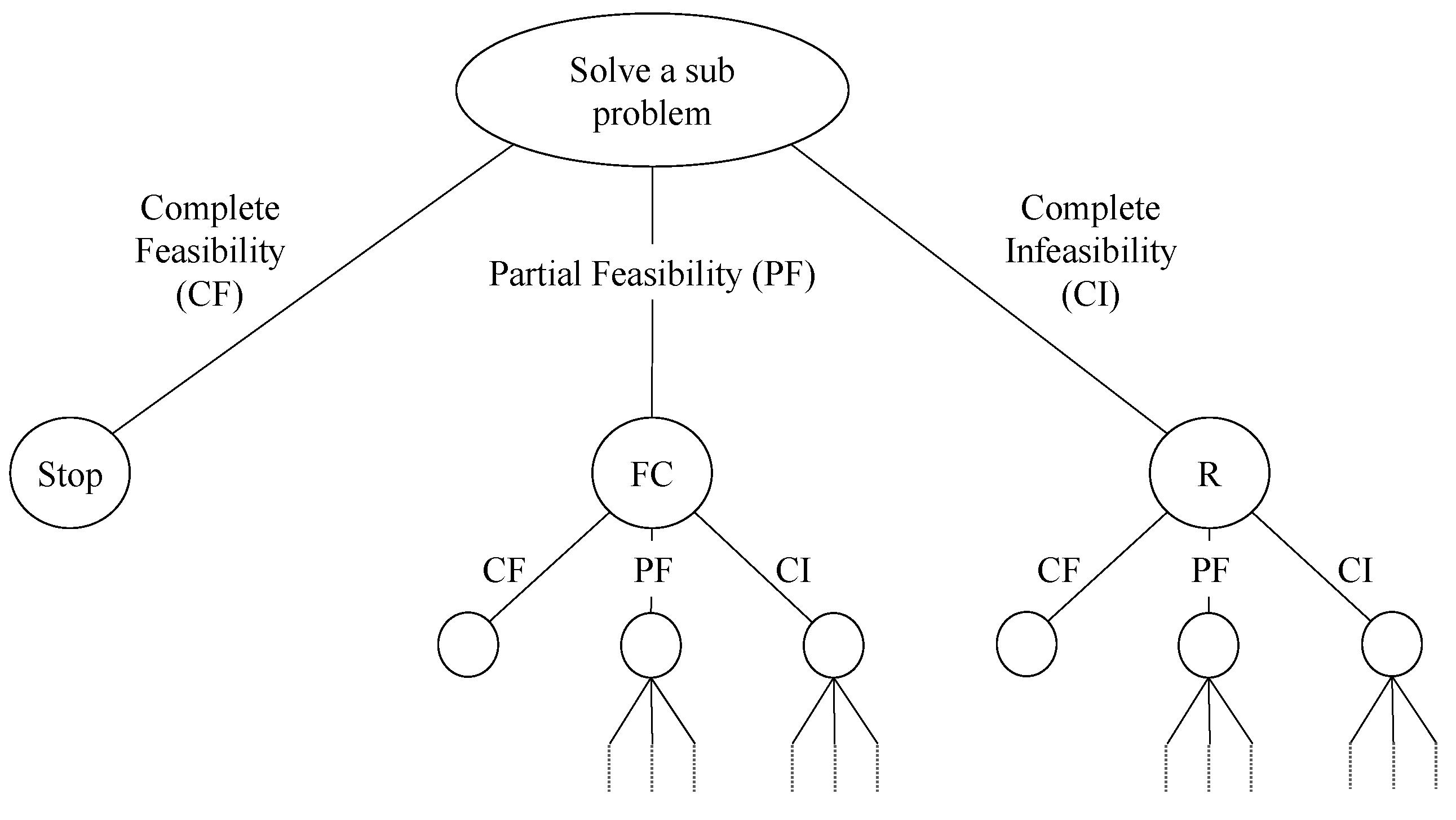
5.1. Conceptual View of the Proposed Algorithm

The algorithm introduced in this section is referred to as the branch-and-freeze (BF) algorithm. The logical idea behind the BF algorithm is to solve relaxed problems (sub-problems) of the original problem in a manner similar to the branch-and-bound method. We observed that the MOQ and MPA constraints in Equations (15)–(18) are computationally burdensome because of the binary variables involved and the large number of constraints, amounting to the total $2IKT+KT$. Based on this observation, the sub-problems are created by removing the MOQ and MPA constraints of the original problem, MIP1. When the sub-problem is solved, one of three cases can occur, as illustrated in Figure 1.

The first of the three cases is that a solution to a sub-problem also satisfies the MOQ and MPA constraints of all suppliers, which we call complete feasibility (CF) case. In Figure 1 below, the CF case is represented by the left-most branch. In this case, the solution is also optimal to MIP1. Since, the original problem is solved optimally, the algorithm stops. The second case occurs when the MOQ and MPA constraints are satisfied partially, which is the situation where the solution to a sub-problem satisfies the two constraints of all suppliers up to a certain intermediate period, but not to the end of the planning horizon. This case is named partial feasibility (PF). When PF occurs, the algorithm stores the current output up to the satisfied period, which is called freezing. For the remaining periods that are not frozen, a new condensed problem is generated by adding the MOQ and MPA constraints of the supplier(s) whose constraints were violated in the previous run. In Figure 1 below, this process is denoted by the circle with FC (freezing and condensing). When the condensed problem is solved afterwards, it results in one of the three cases already explained above.

The final case, which is in the right most side of Figure 1, is the complete infeasibility (CI) case, where the sub-problem’s output can satisfy none of the suppliers’ MOQ and MPA constraints, even at the starting period. If this happens, a new sub-problem is created by adding all of the removed constraints. This process is denoted by a circle with an R (restoring) inside. When a restored problem is solved, one of the same three cases can occur. A node is fathomed when the stop condition is met after CF, or no additional constraint is available for addition after PF or CI. The best feasible solution to the original problem is the best feasible solution found until all end nodes are fathomed. If there is no feasible solution found up to that point, the original problem is infeasible.

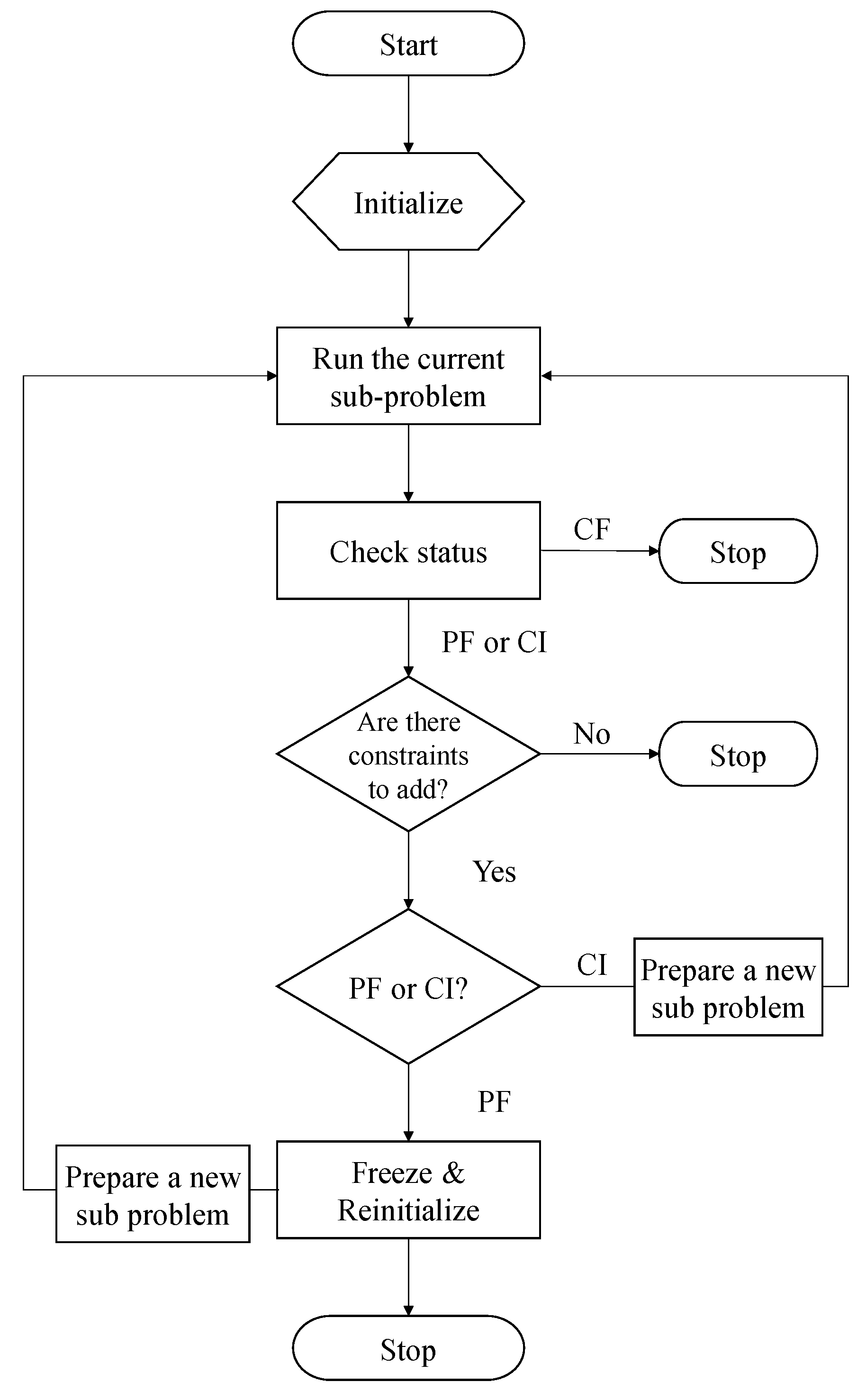
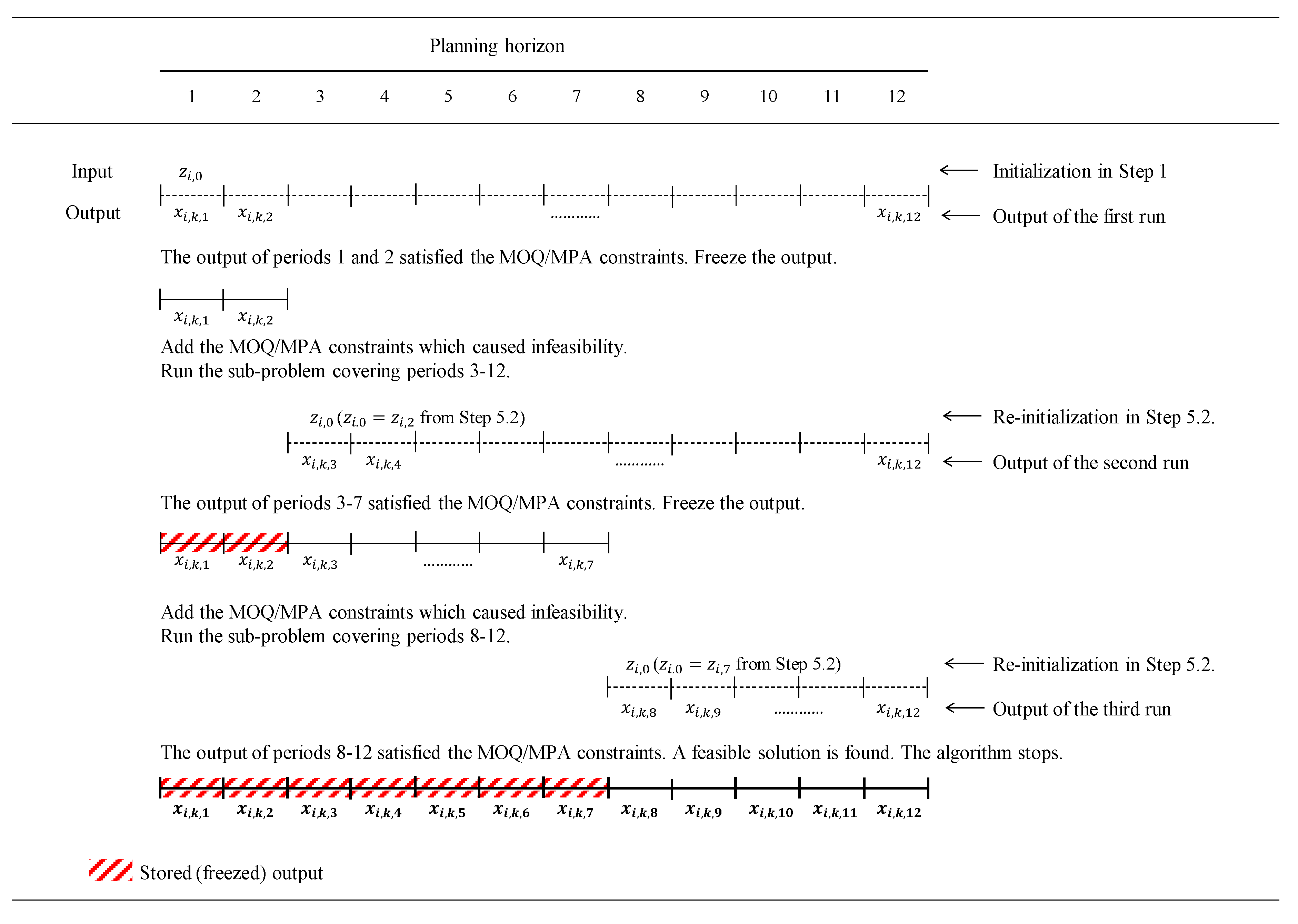
5.2. Branch-and-Freeze (BF) Algorithm

The BF algorithm can be described formally as follows:

Step 1: (Initialize)

Let the current period be period 1.

Set the current inventory level, $z_{i,0}=0$ for $i=1,2,\cdots ,I$.

Forecast demand for all future periods, $d_{i,t}$ for $t=1,2,\cdots ,T$.

Step 2: (Generate sub-problem for the first run)

Construct the sub-problem by removing the MOQ and MPA constraints (Equations (15)–(18) from MIP1).

Step 3: (Run sub-problem)

Run the current sub-problem.

Step 4: (Check status and branch)

Step 4.1 Check the output of Step 3. If status is PF or CF, go to Step 4.3.

Step 4.2 (Complete feasibility case)

Algorithm found a feasible solution. Stop.

Step 4.3 (Partial feasibility or complete infeasibility case)

If there is no constraint to add, the given problem is infeasible. Stop.

Go to Step 5 if status is PF. Otherwise, go to Step 6.

Step 5: (Partial feasibility case)

Step 5.1 (Freeze the output)

Freeze the output for the feasible periods.

Step 5.2 (Re-initialize)

Let the starting period be the first infeasible period.

Reset the current inventory level to the net inventory level of the last feasible period.

Reset the forecast of demand from the starting to the end periods of the planning horizon.

Step 5.3 (Prepare a sub-problem)

Prepare a new sub-problem by adding the MOQ or MPA constraints of the supplier(s), which caused infeasibility during the previous run. Go to Step 3.

Step 6: (Complete Infeasibility case)

Prepare a new sub-problem by adding the MOQ or MPA constraints of the supplier(s), which caused infeasibility during the previous run. Go to Step 3.

Step 1 is for the initialization required for the first planning run. The constraint relaxation that is required to solve MIP1 without the MOQ and MPA constraints is done in Step 2. After initialization and relaxation, a relaxed version of MIP1 (sub-problem) is solved in Step 3. In Step 4, the output of the previous run is evaluated for status. Based on the status, the algorithm stops or proceeds to Steps 5 or 6 when there is (are) a constraint(s) to add. Figure 2 shows the flow of the algorithm. Figure 3 illustrates an implementation of the algorithm.

6. Numerical Experiments

In this chapter, numerical experiments are carried out with two objectives in mind. The first objective of the numerical experiment is to test the accuracy of the BF algorithm by comparing it with a commercially available software tool (GAMS/XPRESS solver). The second experiment explores the maximum size of MIP1 that can be solved by the BF algorithm and by commercial software tools (GAMS/XPRESS and GAMS/COINGLPK solvers). The results of these two numerical experiments will determine the effectiveness of the BF algorithm. The GAMS used in the numerical experiment is a very popular modeling language containing many powerful solvers. Thus, it is a suitable competitor for verifying the accuracy and identifying the maximum solvable problem size of the BF algorithm. The experiments were performed on a PC with Microsoft 7 OS, 3.4GHz Intel i5 CPU, and 16 GB RAM.

6.1. Accuracy Test of the BF Algorithm

The purpose of this experiment is to identify the accuracy of the BF algorithm by comparing the results obtained using our algorithm with those of the GAMS/XPRESS solver. The comparative experiment is performed with the assumption that the item’s demand is generated from a stationary demand process. Most previous studies on inventory management performed experiments by assuming that demand follows a stationary demand process, such as a Poisson or normal distribution [56]. For our problem, many relevant studies, including Robb and Silver [18], Chen et al. [57], and Zhou [22], also assumed a normal distribution. This experiment is also carried out similarly by assuming a normal distribution assumption. The number of item types is set to five. The actual demand data for each item were generated from five different normal distributions $(N(400,{20}^2),N(600,{30}^2),N(700,{40}^2),N(800,{40}^2),N(900,{50}^2))$. Each item’s demand forecast is prepared using the forecasting module of SPSS.

To obtain the average total cost, the experiment was repeated 10 times for each setting. The average cost obtained in this manner is plugged into the following percent deviation measure to identify the accuracy of the BF algorithm.

$$\mathrm{Percent}\mathrm{deviation}=\frac{{\mathrm{BF}\mathrm{algorithm}}^{’}\cos \mathrm{t}-{\mathrm{GAMS}}^{’}\cos \mathrm{t}}{{\mathrm{GAMS}}^{’}\cos \mathrm{t}}\times 100.$$

The experimental design is as follows:

• There are 10 suppliers in the system.
• Transportation lead time is zero.
• Each supplier can deliver all five types of items.
• The unit period length is four weeks.
• The planning horizon length is sized to 48 weeks, which amounts to 1 year.

Other input parameters were prepared as shown in

Table 2. Input parameters for the comparative experiment.

$\mathbf{Warehouse}\mathbf{Capacity}\mathbf{of}\mathbf{Buyer}(\mathit{w}{\mathit{c}}_{\mathit{t}})$	$\mathbf{Very}\mathbf{Large}\mathbf{Number}(\mathit{M})$	$\mathbf{Discount}\mathbf{Factor}(\mathit{r})$	$\mathbf{Initial}\mathbf{Inventory}\mathbf{Level}(\mathit{I}{\mathit{P}}_{\mathit{i}0})$
5000.00	${10}^7$	0.01	0

,

Table 3. Input parameters for each item.

Item	$\mathbf{Holding}\mathbf{Cos}\mathit{t}({\mathit{h}}_{\mathit{i}})$	$\mathbf{Shortage}\mathbf{Cost}({\mathit{b}}_{\mathit{i}})$	$\mathbf{Volume}({\mathit{v}}_{\mathit{i}})$	$\mathbf{Spot}\mathbf{Market}\mathbf{Price}({\mathit{p}}_{\mathit{i}\mathit{t}}^{\mathit{s}})$
All items	$N(2,{0.1}^2)$	$N(15,1^2)$	2.00	$N(27,1^2)$

$N$ denotes a normal distribution.

,

Table 4. Input parameters for each supplier.

Supplier	$\mathbf{Minimum}\mathbf{Purchase}\mathbf{Amount}(\mathit{m}\mathit{p}{\mathit{a}}_{\mathit{k}})$	$\mathbf{Major}\mathbf{Ordering}\mathbf{Cost}(\mathit{m}{\mathit{a}}_{\mathit{k}})$
All suppliers	$20\times 1.0\times \widehat{d}$	$N(250,{10}^2)$

$\widehat{d}$ is the forecast average for the planning horizon.

,

Table 5. Input parameters for each item of each supplier.

Supplier	$\mathbf{Minimum}\mathbf{Order}\mathbf{Quantity}(\mathit{m}\mathit{p}{\mathit{a}}_{\mathit{i}\mathit{k}})$	$\mathbf{Minor}\mathbf{Ordering}\mathbf{Cost}(\mathit{m}{\mathit{i}}_{\mathit{i}\mathit{k}})$
	Item 1 to 5	Item 1 to 5
All suppliers	$N(1,{0.2}^2)\times \widehat{d_i}$	$N(1.5,{0.2}^2)$

$\widehat{d_j}$ denotes the average of forecasts for item $j$ at the planning horizon.

and

Table 6. Input parameters for each period.

Supplier	$\mathbf{Purchase}\mathbf{Price}({\mathit{p}}_{\mathit{i}\mathit{k}\mathit{t}})\mathbf{for}\mathbf{All}\mathbf{Period}$	$\mathbf{Maximum}\mathbf{Purchase}\mathbf{Limit}(\mathit{m}\mathit{p}{\mathit{l}}_{\mathit{i}\mathit{k}})\mathbf{for}\mathbf{All}\mathbf{Period}$
	Item 1 to 5	Item 1 to 5
All suppliers	$N(20,1^2)$	$N(3,{0.5}^2)\times \widehat{d_i}$

.

The results of the first experiment are summarized in

Table 7. Summary of the accuracy test results.

Method	Average Annual Discounted Cost	Average Percent Deviation (%)	Standard Deviation of Percent Deviation	Average CPU Time	Average Number of Sub-Problems Solved
GAMS	$805,041.43	-	-	1.467 s	-
BF algorithm	$811,630.50	0.82%	0.34%	2.920 s	5.5

. Using the BF algorithm instead of commercial solvers (GAMS/XPRESS solver), the average total discounted cost increased by 0.82%. The reason for this was the inventory and shortage appearing at the end of the planning horizon. However, the proposed BF algorithm can offer a result very close to the optimum solution. Thus, it seems that the BF algorithm is able to find a near-optimal solution, even though it is a heuristic algorithm mainly developed to solve larger instances of the problem which cannot be solved by any other existing tools.

6.2. Experiment to Estimate the Maximum Solvable Problem Size of the BF Algorithm

Various software tools developed to solve optimization models have a maximum size limit on the problem which can be solved within a reasonable computational time. Considering this limitation, we attempted to estimate the maximum problem size that can be solved by the BF algorithm. More specifically, the maximum size of problems that can be solved by commercial software tools and the BF algorithm was estimated for comparison. In the experiment, GAMS/XPRESS and GAMS/COINGLPK solvers were selected for comparison. The planning horizon of the problem was fixed to 12 time periods, and the number of suppliers was set to 10 times the number of items. The maximum computational time limit was set to 24 h. We increased the number of items until each method could not find a solution within the time limit. Other input parameters were set as shown in Section 5.1 (Table 2, Table 3, Table 4, Table 5 and Table 6), and demand data were generated using a normal distribution.

The results of the experiment are summarized in

Table 8. Summary of the results for the maximum problem size test.

GAMS Solver	Size of the Problem That Can Be Solved (Number of Items, Number of Constraints, and Number of Variables)
	GAMS Solver	BF Algorithm
COINGLPK	(12, 92,688, 56,928)	(17, 182,268, 111,233)
XPRESS	(69, 2,892,300, 1,743,045)	(108, 7,054,224, 4,244,544)

, and show that the BF algorithm could considerably increase the solvable problem size. The BF algorithm using the COINGLPK to solve sub-problems can double the solvable problem size compared with a naive use of the COINGLPK. Moreover, for the XPRESS case, the size increased approximately 2.4 times in terms of the number of constraints. Thus, it is expected that buyers will be aided in effective decision-making upon using this method for solving real-world complex problems.

7. Managerial Implications

7.1. Academic Implications

In this paper, we studied a sustainable supplier selection and order allocation problem. This is the first attempt to develop a model for the most realistic and complicated SSS & OA problem representing various important features of a real system. A new algorithm specifically designed to solve such a large-scale model is developed. The algorithm performed as expected by increasing solvable problem size considerably. In this way, we have done some initiating academic research in SSS & OA that will help researchers study related follow-up problems.

7.2. Managerial Implications

This study provides valuable insights for firms that regularly make a supplier selection and order allocation decisions. The model and solution method of this paper helps managers to make the SSS & OA decision more systematically. They can prepare a cost-minimizing plan quickly and easily after they complete a computerized planning system. The model is flexible and customizable, and can be modified based on the actual needs of a firm. Output of the developed system provides an efficient SSS & OA plan and, also, some useful additional information, which can be used for many what-if analyses. For example, the dual price of Equation (19) is an incremental cost for raising the 3BL target value by one unit. A firm trying to achieve more stringent sustainability performance can use the estimated cost to make an investment decision for improving a production or logistics system for better sustainability. Thus, good implementation of the model and algorithm of this research will result in better decisions on reducing costs, increasing profitability, and improving customer service sustainability. The final result will be enhanced competitiveness and improved financial status.

8. Conclusions

This paper presents models representing an SSS & OA problem for a buyer replenishing from two or more heterogeneous suppliers with MOQ and MPA constraints, operating working capital limits, and a 3BL sustainability target requirement. A mixed-integer programming model can find a cost-minimizing SSS & OA plan of choosing order-fulfilling suppliers and allocate the order amount for each select supplier. Since the size of a completed model for a real-life application is too big to implement it naively, a fast heuristic algorithm, called a BF algorithm, was also developed for such a large-scale implementation.

The logical idea behind the BF algorithm is two-fold, relaxation and branching. Observing that the MOQ and MPA constraints of the model are very computationally burdensome because of the binary variables included and large number of constraints involved, the algorithm creates sub-problems by relaxing (removing) the MOQ and MPA constraints of the original problem. When the sub-problem is created, a procedure similar to the branch-and-bound method is employed to solve the sub-problems efficiently. Several types of experiments were conducted using the GAMS solvers and IBM SPSS statistics package to verify the validity of the proposed model and to test the accuracy of the developed algorithm. The test result confirmed that the algorithm can find a near-optimal solution with only 0.82 percent deviation on average.

Another test was done to find how much larger a model can be solved when using the proposed algorithm compared with a direct one-time use of popular commercial solvers. The test result showed that the use of the BF algorithm can increase solvable problem size by as much as 2.4 times. It was verified that a model with 7 million constraints and 9 million variables can be handled by our algorithm. All in all, the test results can be summarized as the BF algorithm is an effective tool for handling complex real-life applications. Buyers faced with a large-scale system will, thus, be able to handle such large-scale decision problems without much difficulties.

There are some related research topics that require exploration. Further research may incorporate the supplier’s perspective into the current problem to extend to a supplier–buyer problem. Also, the single objective of the current model can be extended to allow bi- or multi-objective functions to consider quantitative targets and qualitative preferences at the same time. Then, another kind of solution methodology should be developed to solve such a multi-objective optimization model of realistic size. Finally, the current model describes SSS & OA activities in a two-stage supply chain composed of a single buyer and several suppliers. These simple stages can be extended to a more complex case, such as a three-stage model, including another layer of suppliers or manufacturers.

References

1. Ghadimi, P.; Toosi, F.G.; Heavey, C. A multi-agent systems approach for sustainable supplier selection and order allocation in a partnership supply chain. Eur. J. Oper. Res. 2018, 269, 286–301. [Google Scholar] [CrossRef]
2. Fazlollahtabar, H. An integration between fuzzy promethee and fuzzy linear program for supplier selection problem: Case study. J. Appl. Math. Model. Comput. 2016, 1. Available online: http://www.lawarencepress.com/ojs/index.php/JAMMC/article/download/30/543 (accessed on 10 December 2018).
3. Kannan, D. Role of multiple stakeholders and the critical success factor theory for the sustainable supplier selection process. Int. J. Prod. Econ. 2018, 195, 391–418. [Google Scholar] [CrossRef]
4. Kuo, R.; Lee, L.; Hu, T.-L. Developing a supplier selection system through integrating fuzzy ahp and fuzzy dea: A case study on an auto lighting system company in taiwan. Prod. Plan. Control 2010, 21, 468–484. [Google Scholar] [CrossRef]
5. Roehrich, J.K.; Hoejmose, S.U.; Overland, V. Driving green supply chain management performance through supplier selection and value internalisation: A self-determination theory perspective. Int. J. Oper. Prod. Manag. 2017, 37, 489–509. [Google Scholar] [CrossRef]
6. CMMI Product Team. Cmmi for Acquisition; Version 1.3.; Software Engineering Institute: Pittsburgh, PA, USA, 2010. [Google Scholar]
7. ITSqc. Available online: http://www.itsqc.org (accessed on 10 December 2018).
8. Musalem, E.P.; Dekker, R. Controlling inventories in a supply chain: A case study. Int. J. Prod. Econ. 2005, 93, 179–188. [Google Scholar] [CrossRef] [Green Version]
9. Kiesmüller, G.P.; De Kok, A.; Dabia, S. Single item inventory control under periodic review and a minimum order quantity. Int. J. Prod. Econ. 2011, 133, 280–285. [Google Scholar] [CrossRef] [Green Version]
10. Park, J.H.; Kim, J.S.; Shin, K.Y. Inventory control model for a supply chain system with multiple types of items and minimum order size requirements. Int. Trans. Oper. Res. 2018, 25, 1927–1946. [Google Scholar] [CrossRef]
11. Yao, M.; Minner, S. Review of multi-supplier inventory models in supply chain management: An update. 2017. Available online: https://papers.ssrn.com/sol3/papers.cfm?abstract_id=2995134 (accessed on 10 December 2018).
12. Ghorbani, M.; Bahrami, M.; Arabzad, S.M. An integrated model for supplier selection and order allocation; using shannon entropy, swot and linear programming. Procedia Soc. Behav. Sci. 2012, 41, 521–527. [Google Scholar] [CrossRef]
13. Nazari-Shirkouhi, S.; Shakouri, H.; Javadi, B.; Keramati, A. Supplier selection and order allocation problem using a two-phase fuzzy multi-objective linear programming. Appl. Math. Model. 2013, 37, 9308–9323. [Google Scholar] [CrossRef]
14. Jadidi, O.; Cavalieri, S.; Zolfaghari, S. An improved multi-choice goal programming approach for supplier selection problems. Appl. Math. Model. 2015, 39, 4213–4222. [Google Scholar] [CrossRef]
15. Jadidi, O.; Zolfaghari, S.; Cavalieri, S. A new normalized goal programming model for multi-objective problems: A case of supplier selection and order allocation. Int. J. Prod. Econ. 2014, 148, 158–165. [Google Scholar] [CrossRef]
16. Sodenkamp, M.A.; Tavana, M.; Di Caprio, D. Modeling synergies in multi-criteria supplier selection and order allocation: An application to commodity trading. Eur. J. Oper. Res. 2016, 254, 859–874. [Google Scholar] [CrossRef]
17. Shabanpour, H.; Yousefi, S.; Saen, R.F. Future planning for benchmarking and ranking sustainable suppliers using goal programming and robust double frontiers dea. Transp. Res. Part D Transp. Environ. 2017, 50, 129–143. [Google Scholar] [CrossRef]
18. Robb, D.J.; Silver, E.A. Inventory management with periodic ordering and minimum order quantities. J. Oper. Res. Soc. 1998, 49, 1085–1094. [Google Scholar] [CrossRef]
19. Zhao, Y.; Katehakis, M.N. On the structure of optimal ordering policies for stochastic inventory systems with minimum order quantity. Probab. Eng. Inf. Sci. 2006, 20, 257–270. [Google Scholar] [CrossRef]
20. Zhou, B.; Zhao, Y.; Katehakis, M.N. Effective control policies for stochastic inventory systems with a minimum order quantity and linear costs. Int. J. Prod. Econ. 2007, 106, 523–531. [Google Scholar] [CrossRef]
21. Meena, P.; Sarmah, S. Multiple sourcing under supplier failure risk and quantity discount: A genetic algorithm approach. Transp. Res. Part: Logist. Transp. Rev. 2013, 50, 84–97. [Google Scholar] [CrossRef]
22. Zhou, B. Inventory management of multi-item systems with order size constraint. Int. J. Syst. Sci. 2010, 41, 1209–1219. [Google Scholar] [CrossRef]
23. Aktin, T.; Gergin, Z. Mathematical modelling of sustainable procurement strategies: Three case studies. J. f Clean. Prod. 2016, 113, 767–780. [Google Scholar] [CrossRef]
24. Bian, Y.; Lemoine, D.; Yeung, T.G.; Bostel, N.; Hovelaque, V.; Viviani, J.-L.; Gayraud, F. A dynamic lot-sizing-based profit maximization discounted cash flow model considering working capital requirement financing cost with infinite production capacity. Int. J. Prod. Econ. 2018, 196, 319–332. [Google Scholar] [CrossRef]
25. Chen, T.-L.; Lin, J.T.; Wu, C.-H. Coordinated capacity planning in two-stage thin-film-transistor liquid-crystal-display (tft-lcd) production networks. Omega 2014, 42, 141–156. [Google Scholar] [CrossRef]
26. Chao, X.; Chen, J.; Wang, S. Dynamic inventory management with cash flow constraints. Nav. Res. Logist. 2008, 55, 758–768. [Google Scholar] [CrossRef] [Green Version]
27. Bendavid, I.; Herer, Y.T.; Yücesan, E. Inventory management under working capital constraints. J. Simul. 2017, 11, 62–74. [Google Scholar] [CrossRef]
28. Azadnia, A.H.; Saman, M.Z.M.; Wong, K.Y. Sustainable supplier selection and order lot-sizing: An integrated multi-objective decision-making process. Int. J. Prod. Res. 2015, 53, 383–408. [Google Scholar] [CrossRef]
29. Oxford. What Is a Pestel Analysis? Available online: https://blog.oxfordcollegeofmarketing.com/2016/06/30/pestel-analysis/ (accessed on 10 December 2018).
30. Handfield, R.; Walton, S.V.; Sroufe, R.; Melnyk, S.A. Applying environmental criteria to supplier assessment: A study in the application of the analytical hierarchy process. Eur. J. Oper. Res. 2002, 141, 70–87. [Google Scholar] [CrossRef]
31. Lu, L.Y.; Wu, C.; Kuo, T.-C. Environmental principles applicable to green supplier evaluation by using multi-objective decision analysis. Int. J. Prod. Res. 2007, 45, 4317–4331. [Google Scholar] [CrossRef]
32. Lee, A.H.; Kang, H.-Y.; Hsu, C.-F.; Hung, H.-C. A green supplier selection model for high-tech industry. Expert Syst. Appl. 2009, 36, 7917–7927. [Google Scholar] [CrossRef]
33. Hsu, C.-W.; Hu, A.H. Applying hazardous substance management to supplier selection using analytic network process. J. Clean. Prod. 2009, 17, 255–264. [Google Scholar] [CrossRef]
34. Kannan, G.; Pokharel, S.; Kumar, P.S. A hybrid approach using ism and fuzzy topsis for the selection of reverse logistics provider. Resour. Conserv. Recycl. 2009, 54, 28–36. [Google Scholar] [CrossRef]
35. Yeh, W.-C.; Chuang, M.-C. Using multi-objective genetic algorithm for partner selection in green supply chain problems. Expert Syst. Appl. 2011, 38, 4244–4253. [Google Scholar] [CrossRef]
36. Büyüközkan, G.; Çifçi, G. A novel hybrid mcdm approach based on fuzzy dematel, fuzzy anp and fuzzy topsis to evaluate green suppliers. Expert Syst. Appl. 2012, 39, 3000–3011. [Google Scholar] [CrossRef]
37. Shaw, K.; Shankar, R.; Yadav, S.S.; Thakur, L.S. Supplier selection using fuzzy ahp and fuzzy multi-objective linear programming for developing low carbon supply chain. Expert Syst. Appl. 2012, 39, 8182–8192. [Google Scholar] [CrossRef]
38. Govindan, K.; Khodaverdi, R.; Jafarian, A. A fuzzy multi criteria approach for measuring sustainability performance of a supplier based on triple bottom line approach. J. Clean. Prod. 2013, 47, 345–354. [Google Scholar] [CrossRef]
39. Shen, L.; Olfat, L.; Govindan, K.; Khodaverdi, R.; Diabat, A. A fuzzy multi criteria approach for evaluating green supplier’s performance in green supply chain with linguistic preferences. Resour. Conserv. Recycl. 2013, 74, 170–179. [Google Scholar] [CrossRef]
40. Dobos, I.; Vörösmarty, G. Green supplier selection and evaluation using dea-type composite indicators. Int. J. Prod. Econ. 2014, 157, 273–278. [Google Scholar] [CrossRef]
41. Kannan, D.; Govindan, K.; Rajendran, S. Fuzzy axiomatic design approach based green supplier selection: A case study from singapore. J. Clean. Prod. 2015, 96, 194–208. [Google Scholar] [CrossRef]
42. Awasthi, A.; Kannan, G. Green supplier development program selection using ngt and vikor under fuzzy environment. Comput. Ind. Eng. 2016, 91, 100–108. [Google Scholar] [CrossRef]
43. Trapp, A.C.; Sarkis, J. Identifying robust portfolios of suppliers: A sustainability selection and development perspective. J. Clean. Prod. 2016, 112, 2088–2100. [Google Scholar] [CrossRef]
44. Qin, J.; Liu, X.; Pedrycz, W. An extended todim multi-criteria group decision making method for green supplier selection in interval type-2 fuzzy environment. Eur. J. Oper. Res. 2017, 258, 626–638. [Google Scholar] [CrossRef]
45. Gupta, H.; Barua, M.K. Supplier selection among smes on the basis of their green innovation ability using bwm and fuzzy topsis. J. Clean. Prod. 2017, 152, 242–258. [Google Scholar] [CrossRef]
46. Luthra, S.; Govindan, K.; Kannan, D.; Mangla, S.K.; Garg, C.P. An integrated framework for sustainable supplier selection and evaluation in supply chains. J. Clean. Prod. 2017, 140, 1686–1698. [Google Scholar] [CrossRef]
47. Yu, F.; Yang, Y.; Chang, D. Carbon footprint based green supplier selection under dynamic environment. J. Clean. Prod. 2018, 170, 880–889. [Google Scholar] [CrossRef]
48. Banaeian, N.; Mobli, H.; Fahimnia, B.; Nielsen, I.E.; Omid, M. Green supplier selection using fuzzy group decision making methods: A case study from the agri-food industry. Comput. Oper. Res. 2018, 89, 337–347. [Google Scholar] [CrossRef]
49. Kannan, D.; Khodaverdi, R.; Olfat, L.; Jafarian, A.; Diabat, A. Integrated fuzzy multi criteria decision making method and multi-objective programming approach for supplier selection and order allocation in a green supply chain. J. Clean. Prod. 2013, 47, 355–367. [Google Scholar] [CrossRef]
50. Govindan, K.; Jafarian, A.; Nourbakhsh, V. Bi-objective integrating sustainable order allocation and sustainable supply chain network strategic design with stochastic demand using a novel robust hybrid multi-objective metaheuristic. Comput. Oper. Res. 2015, 62, 112–130. [Google Scholar] [CrossRef]
51. Gören, H.G. A decision framework for sustainable supplier selection and order allocation with lost sales. J. Clean. Prod. 2018, 183, 1156–1169. [Google Scholar] [CrossRef]
52. Ayhan, M.B.; Kilic, H.S. A two stage approach for supplier selection problem in multi-item/multi-supplier environment with quantity discounts. Comput. Ind. Eng. 2015, 85, 1–12. [Google Scholar] [CrossRef]
53. Yang, Y.H.; Kim, J.S. An adaptive joint replenishment policy for items with non-stationary demands. Oper. Res. 2018, 1–20. [Google Scholar] [CrossRef]
54. Theodore Farris, M.; Hutchison, P.D. Cash-to-cash: The new supply chain management metric. Int. J. Phys. Distrib. Logist. Manag. 2002, 32, 288–298. [Google Scholar] [CrossRef]
55. Hofmann, E.; Kotzab, H. A supply chain-oriented approach of working capital management. J. Bus. Logist. 2010, 31, 305–330. [Google Scholar] [CrossRef]
56. Agrawal, N.; Smith, S.A. Estimating negative binomial demand for retail inventory management with unobservable lost sales. Nav. Res. Logist. 1996, 43, 839–861. [Google Scholar] [CrossRef]
57. Chen, J.; Zhao, X.; Zhou, Y. A periodic-review inventory system with a capacitated backup supplier for mitigating supply disruptions. Eur. J. Oper. Res. 2012, 219, 312–323. [Google Scholar] [CrossRef]
Figure 1. Conceptual view of the branch-and-freeze (BF) algorithm.
Mathematics 06 00325 g001
Figure 2. Flow chart of the BF algorithm.
Mathematics 06 00325 g002
Figure 3. Implementation diagram of the BF algorithm.
Mathematics 06 00325 g003