Hybrid Second Order Method for Orthogonal Projection onto Parametric Curve in n-Dimensional Euclidean Space

Abstract

Orthogonal projection a point onto a parametric curve, three classic first order algorithms have been presented by Hartmann (1999), Hoschek, et al. (1993) and Hu, et al. (2000) (hereafter, H-H-H method). In this research, we give a proof of the approach’s first order convergence and its non-dependence on the initial value. For some special cases of divergence for the H-H-H method, we combine it with Newton’s second order method (hereafter, Newton’s method) to create the hybrid second order method for orthogonal projection onto parametric curve in an n-dimensional Euclidean space (hereafter, our method). Our method essentially utilizes hybrid iteration, so it converges faster than current methods with a second order convergence and remains independent from the initial value. We provide some numerical examples to confirm robustness and high efficiency of the method.

1. Introduction

In this research, we will discuss the minimum distance problem between a point and a parametric curve in an n-dimensional Euclidean space, and how to gain the closest point (footpoint) on the curve as well as its corresponding parameter, which is termed as the point projection or inversion problem of a parametric curve in an n-dimensional Euclidean space. It is an important issue in the themes such as geometric modeling, computer graphics, computer-aided geometry design (CAGD) and computer vision [1,2]. Both projection and inversion are fundamental for a series of techniques, for instance, the interactive selection of curves and surfaces [1,3], the curve fitting [1,3], reconstructing curves [2,4,5] and projecting a space curve onto a surface [6]. This vital technique is also used in the ICP (iterative closest point) method for shape registration [7].

The Newton-Raphson algorithm is deemed as the most classic one for orthogonal projection onto parametric curve and surface. Searching the root of a polynomial by a Newton-Raphson algorithm can be found in [8,9,10,11,12]. In order to solve the adaptive smoothing for the standard finite unconstrained minimax problems, Polak et al. [13] have presented a extended Newton’s algorithm where a new feedback precision-adjustment rule is used in their extended Newton’s algorithm. Once the Newton-Raphson method reaches its convergence, two advantages emerge and it converges very fast with high precision. However, the result relies heavily on a good guess of initial value in the neighborhood of the solution.

Meanwhile, the classic subdivision method consists of several procedures: Firstly, subdivide NURBS curve or surface into a set of Bézier sub-curves or patches and eliminate redundancy or unnecessary Bézier sub-curves or Bézier patches. Then, get the approximation candidate points. Finally, get the closest point through comparing the distances between the test point and candidate points. This technique is reflected in [1]. Using new exclusion criteria within the subdivision strategy, the robustness for the projection of points on NURBS curves and surfaces in [14] has been improved than that in [1], but this criterion is sometimes too critical. Zou et al. [15] use subdivision minimization techniques which rely on the convex hull characteristic of the Bernstein basis to impute the minimum distance between two point sets. They transform the problem into solving of n-dimensional nonlinear equations, where n variables could be represented as the tensor product Bernstein basis. Cohen et al. [16] develop a framework for implementing general successive subdivision schemes for nonuniform B-splines to generate the new vertices and the new knot vectors which are satisfied with derived polygon. Piegl et al. [17] repeatedly subdivide a NURBS surface into four quadrilateral patches and then project the test point onto the closest quadrilateral until it can find the parameter from the closest quadrilateral. Using multivariate rational functions, Elber et al. [11] construct a solver for a set of geometric constraints represented by inequalities. When the dimension of the solver is greater than zero, they subdivide the multivariate function(s) so as to bind the function values within a specified domain. Derived from [11] but with more efficiency, a hybrid parallel method in [18] exploits both the CPU and the GPU multi-core architectures to solve systems under multivariate constraints. Those GPU-based subdivision methods essentially exploit the parallelism inherent in the subdivision of multivariate polynomial. This geometric-based algorithm improves in performance compared to the existing subdivision-based CPU. Two blending schemes in [19] efficiently remove no-root domains, and hence greatly reduce the number of subdivisions. Through a simple linear combination of functions for a given system of nonlinear equations, no-root domain and searching out all control points for its Bernstein-Bézier basic with the same sign must be satisfied with the seek function. During the subdivision process, it can continuously create these kinds of functions to get rid of the no-root domain. As a result, van Sosin et al. [20] efficiently form various complex piecewise polynomial systems with zero or inequality constraints in zero-dimensional or one-dimensional solution spaces. Based on their own works [11,20], Bartoň et al. [21] propose a new solver to solve a non-constrained (piecewise) polynomial system. Two termination criteria are applied in the subdivision-based solver: the no-loop test and the single-component test. Once two termination criteria are satisfied, it then can get the domains which have a single monotone univariate solution. The advantage of these methods is that they can find all solutions, while their disadvantage is that they are computationally expensive and may need many subdivision steps.

The third classic methods for orthogonal projection onto parametric curve and surface are geometry methods. They are mainly classified into eight different types of geometry methods: tangent method [22,23], torus patch approximating method [24], circular or spherical clipping method [25,26], culling technique [27], root-finding problem with Bézier clipping [28,29], curvature information method [6,30], repeated knot insertion method [31] and hybrid geometry method [32]. Johnson et al. [22] use tangent cones to search for regions with satisfaction of distance extrema conditions and then to solve the minimum distance between a point and a curve, but it is not easy to construct tangent cones at any time. A torus patch approximatively approaches for point projection on surfaces in [24]. For the pure geometry method of a torus patch, it is difficult to achieve high precision of the final iterative parametric value. A circular clipping method can remove the curve parts outside a circle with the test point being the circle’s center, and the radius of the elimination circle will shrink until it satisfies the criteria to terminate [26]. Similar to the algorithm [26], a spherical clipping technique for computing the minimum distance with clamped B-spline surface is provided by [25]. A culling technique to remove superfluous curves and surfaces containing no projection from the given point is proposed in [27], which is in line with the idea in [1]. Using Newton’s method for the last step [1,25,26,27], the special case of non-convergence may happen. In view of the convex-hull property of Bernstein-Bézier representations, the problem to be solved can be formulated as a univariate root-finding problem. Given a $C^1$ parametric curve $c\left(t\right)$ and a point p, the projection constraint problem can be formulated as a univariate root-finding problem $⟨c^{\prime }\left(t\right),c\left(t\right)-p⟩=0$ with a metric induced by the Euclidean scalar product in $R^n$. If the curve is parametrized by a (piece-wise) polynomial, then the fast root-finding schemes as a Bézier clipping [28,29] can be used. The only issue is the $C^1$ discontinuities that can be checked in a post-process. One advantage of these methods is that they do not need any initial guess on the parameter value. They adopt the key technology of degree reduction via clipping to yield a strip bounded of two quadratic polynomials. Curvature information is found for computing the minimum distance between a point and a parameter curve or surface in [6,30]. However, it needs to consider the second order derivative and the method [30] is not fit for n-dimensional Euclidean space. Hu et al. [6] have not proved the convergence of their two algorithms. Li et al. [33] have strictly proved convergence analysis for orthogonal projection onto planar parametric curve in [6]. Based on repeated knot insertion, Mørken et al. [31] exploit the relationship between a spline and its control polygon and then present a simple and efficient method to compute zeros of spline functions. Li et al. [32] present the hybrid second order algorithm which orthogonally projects onto parametric surface; it actually utilizes the composite technology and hence converges nicely with convergence order being 2. The geometric method can not only solve the problem of point orthogonal projecting onto parametric curve and surface but also compute the minimum distance between parametric curves and parametric surfaces. Li et al. [23] have used the tangent method to compute the intersection between two spatial curves. Based on the methods in [34,35], they have extended to compute the Hausdorff distance between two B-spline curves. Based on matching a surface patch from one model to the other model which is the corresponding nearby surface patch, an algorithm for solving the Hausdorff distance between two freeform surfaces is presented in Kim et al. [36], where a hierarchy of Coons patches and bilinear surfaces that approximate the NURBS surfaces with bounding volume is adopted. Of course, the common feature of geometric methods is that the ultimate solution accuracy is not very high. To sum up, these algorithms have been proposed to exploit diverse techniques such as Newton’s iterative method, solving polynomial equation roots methods, subdividing methods, geometry methods. A review of previous algorithms on point projection and inversion problem is obtained in [37].

More specifically, using the tangent line or tangent plane with first order geometric information, a classical simple and efficient first order algorithm which orthogonally project onto parametric curve and surface is proposed in [38,39,40] (H-H-H method). However, the proof of the convergence for the H-H-H method can not be found in this literature. In this research, we try to give two contributions. Firstly, we give proof that the algorithm is first order convergent and it does not depend on the initial value. We then provide some numerical examples to show its high convergence rate. Secondly, for several special cases where the H-H-H method is not convergent, there are two methods (Newton’s method and the H-H-H method) to combine our method. If the H-H-H method’s iterative parametric value is satisfied with the convergence condition of the Newton’s method, we then go to Newton’s method to increase the convergence process. Otherwise, we go on the H-H-H method until its iterative parametric value is satisfied with the convergence condition of the Newton’s method, and we then turn to it as above. This algorithm not only ensures the robustness of convergence, but also improves the convergence rate. Our hybrid method can go faster than the existing methods and ensures the independence to the initial value. Some numerical examples verify our conclusion.

The rest of this paper is arranged as follows. In Section 2, convergence analysis of the H-H-H method is presented. In Section 3, for several special cases where the H-H-H method is not convergent, an improved our method is provided. Convergence analysis for our method is also provided in this section. In Section 4, some numerical examples for our method are verified. In Section 5, conclusions are provided.

2. Convergence Analysis of the H-H-H Method

In this part, we will prove that the algorithm defined by Equations (2) or (3) is of first order convergence and its convergence does not rely on the initial value. Suppose a $C^2$ curve $c\left(t\right)=(f_1\left(t\right),f_2\left(t\right),\dots ,f_n\left(t\right))$ in an n-dimensional Euclidean space ${\mathrm{R}}^n(n\ge 2)$ and a test point $p=(p_1,p_2,\dots ,p_n)$. The first order geometric method to compute the footpoint q of test point p can be implemented as below. Projecting test point p onto the tangent line of the parametric curve $c\left(t\right)$ in an n-dimensional Euclidean space at $t=t_m$ gets a point q determined by $c\left(t_m\right)$ and its derivative $c^{\prime }\left(t_m\right)$. The footpoint can be approximated as

$$q=c\left(t_m\right)+\mathsf{\Delta }t{c}^{\prime }\left(t_m\right).$$

(1)

Then,

$$\mathsf{\Delta }t=\frac{⟨c^{\prime }\left(t_m\right),p-c\left(t_m\right)⟩}{⟨c^{\prime }\left(t_m\right),c^{\prime }\left(t_m\right)⟩},$$

(2)

where $⟨x,y⟩$ is the scalar product of vectors $x,y\in {\mathrm{R}}^n$. Equation (2) can also be expressed as

$$K_1\left(t_m\right)=t_m+\frac{⟨c^{\prime }\left(t_m\right),p-c\left(t_m\right)⟩}{⟨c^{\prime }\left(t_m\right),c^{\prime }\left(t_m\right)⟩}.$$

(3)

Let $t_m\leftarrow K_1\left(t_m\right)$, and repeatedly iterate the above process until $\left|K_1\left(t_m\right)-t_m\right|$ is less than an error tolerance $\epsilon$. This method is addressed as H-H-H method [38,39,40]. Furthermore, convergence of this method will not depend on the choice of the initial value. According to many of our test experiments, when the iterative parametric value approaches the target parametric value $\alpha$, the iteration step size becomes smaller and smaller, while the corresponding number of iterations becomes bigger and bigger.

Theorem 1.

The convergence order of the method defined by Equations (2) or (3) is one, and its convergence does not depend on the initial value.

Proof. 

We adopt the numerical analysis method which is equivalent to those in the literature [41,42]. Firstly, we deduce the expression of footpoint q. Suppose that parameter curve $c\left(t\right)$ is a $C^2$ curve in an n-dimensional Euclidean space ${\mathrm{R}}^n(n\ge 2)$, where the corresponding projecting point with parameter $\alpha$ is orthogonal projecting of the test point $p=(p_1,p_2,\dots ,p_n)$ onto the parametric curve $c\left(t\right)$. It is easy to indicate a relational expression

$$⟨p-h,\mathbf{n}⟩=0,$$

(4)

where $h=c\left(\alpha \right)$ and tangent vector $\mathbf{n}=c^{\prime }\left(\alpha \right)$. In order to solve the intersection (footpoint q) between the tangent line, which goes through the parametric curve $c\left(t\right)$ at $t=t_m$, and the perpendicular line, which is determined by the test point p, we try to express the equation of the tangent line as:

$$x=c\left(t_m\right)+c^{\prime }\left(t_m\right)·s,$$

(5)

where $x=(x_1,x_2,\dots ,x_n)$ and s is a parameter. In addition, the vector of line segment both going through the test point p and the point $c\left(t_m\right)$ will be

$$y=p-x,$$

(6)

where $y=(y_1,y_2,\dots ,y_n)$. Because the vector (6) and the tangent vector $c^{\prime }\left(t_m\right)$ of Equation (5) are orthogonal to each other, the current parameter value s of Equation (5) is

$$s_0=\frac{⟨p-c\left(t_m\right),c^{\prime }\left(t_m\right)⟩}{⟨c^{\prime }\left(t_m\right),c^{\prime }\left(t_m\right)⟩}.$$

(7)

Substituting (7) into (5), we have

$$q=c\left(t_m\right)+c^{\prime }\left(t_m\right)·s_0.$$

(8)

Thus, the footpoint $q=(q_1,q_2,\dots ,q_n)$ is determined by Equation (8).

Secondly, we deduce that the convergence order of the method defined by (2) or (3) is first order convergent. Our proof method absorbs the idea of [41,42]. Substituting (8) into (2), and simplifying, we get the relationship,

$$\mathsf{\Delta }t=\frac{⟨p-c\left(t_m\right),c^{\prime }\left(t_m\right)⟩}{⟨c^{\prime }\left(t_m\right),c^{\prime }\left(t_m\right)⟩}.$$

(9)

Using Taylor’s expansion, we get

$$c\left(t_m\right)={\mathrm{B}}_0+{\mathrm{B}}_1{e}_m+{\mathrm{B}}_2{e}_m^2+o\left(e_m^3\right),$$

(10)

$$c^{\prime }\left(t_m\right)={\mathrm{B}}_1+{2\mathrm{B}}_2{e}_m+o\left(e_m^2\right),$$

(11)

where $e_m=t_m-\alpha$, and ${\mathrm{B}}_i=(1/i!)c^{\left(i\right)}\left(\alpha \right),i=0,1,2,\dots$ From (10) and (11) and combining with (4), the numerator of Equation (9) can be transformed into the following one:

$$\begin{array}{c}⟨p-c\left(t_m\right),c^{\prime }\left(t_m\right)⟩\hfill \\ =L_1{e}_m+L_2{e}_m^2+o\left(e_m^3\right),\hfill \end{array}$$

(12)

where $L_1=2⟨p-{\mathrm{B}}_0,B_{\mathrm{2}}⟩-⟨{\mathrm{B}}_1,{\mathrm{B}}_1⟩,L_2=-3⟨{\mathrm{B}}_1,{\mathrm{B}}_2⟩$. By (11), the denominator of Equation (9) can be changed as follows:

$$\begin{array}{c}⟨c^{\prime }\left(t_m\right),c^{\prime }\left(t_m\right)⟩\hfill \\ =M_1+M_2{e}_m+M_3{e}_m^2+o\left(e_m^3\right),\hfill \end{array}$$

(13)

where $M_1=⟨{\mathrm{B}}_1{,\mathrm{B}}_1⟩,M_2=4⟨{\mathrm{B}}_1{,\mathrm{B}}_2⟩,M_3=4⟨{\mathrm{B}}_2{,\mathrm{B}}_2⟩$. Substituting Equations (12) and (13) into the right-hand side of Equation (9), we get

$$\begin{array}{cc}\hfill \mathsf{\Delta }t=& \frac{⟨p-c\left(t_m\right),c^{\prime }\left(t_m\right)⟩}{⟨c^{\prime }\left(t_m\right),c^{\prime }\left(t_m\right)⟩}\hfill \\ \hfill =& \frac{L_1{e}_m+L_2{e}_m^2+o\left(e_m^3\right)}{M_1+M_2{e}_m+M_3{e}_m^2+o\left(e_m^3\right)}.\hfill \end{array}$$

(14)

Using Taylor’s expansion by Maple 18, and through simplification, we get

$$\begin{array}{cc}\hfill K_1\left(t_m\right)=& \alpha +(\frac{L_1}{M_1}+1)e_m+\frac{L_2{M}_1-L_1{M}_2}{M_1^2}{e}_m^2+o\left(e_m^3\right),\hfill \\ \hfill =& \alpha +(\frac{L_1}{M_1}+1)e_m+o\left(e_m^2\right),\hfill \\ \hfill =& \alpha +C_0{e}_m+o\left(e_m^2\right),\hfill \end{array}$$

(15)

where the symbol $C_0$ is the coefficient of the first order error $e_m$ of Equation (15). The result implies the iterative Equations (2) or (3) is of first order convergence.

Now, we try to interpret that Equations (2) or (3) do not depend on the initial value.

Our proof method absorbs the idea of references [43,44]. Without loss of generality, we only prove that convergence of Equations (2) or (3) does not depend on the initial value in two-dimensional case. As to convergence of Equations (2) or (3) not being dependent on the initial value in general n-dimensional Euclidean space case, it is completely equivalent to the two-dimensional case.

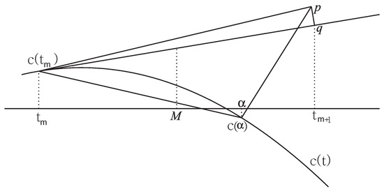
Firstly, we interpret Figure 1. For a horizontal axis t, there are two points are on the planar parametric curve $c\left(t\right)$. For the first point $c\left(t_m\right)$ on the horizontal axis, the test point p orthogonal projects it onto the planar parametric curve $c\left(t\right)$ and yields the second point and its corresponding parameter value $\alpha$ on the horizontal axis. Then, by the iterative methods (2) or (3), the line segment connected by the point p and the point $c\left(\alpha \right)$ is perpendicular to the tangent line of the planar parametric curve $c\left(t\right)$ at $t=\alpha$. The footpoint q is determined by the tangent line of the planar parametric curve $c\left(t\right)$ through the point $c\left(t_m\right)$. Evidently, the parametric value $t_{m+1}$ of footpoint q can be used as the next iterative value. M is the corresponding parametric value of the middle point of the point $c\left(t_m\right)$ and the footpoint q.

Figure 1. Geometric illustration for convergence analysis.

Secondly, we prove the argument whose convergence of Equations (2) or (3) does not depend on the initial value. It is easy to know that t denotes the corresponding parameter for the first dimensional of the planar parametric curve on the two-dimensional plane. When the iterative Equations (2) or (3) start to run, we suppose that the iterative parameter value is satisfied with the inequality relationship $t_m<\alpha$ and the corresponding parameter of the footpoint q is $t_{m+1}$, as shown in Figure 1. The middle point of two points $(t_{m+1},0)$ and $(t_m,0)$ is $(M,0)$, i.e., ${\displaystyle M=\frac{t_m+t_{m+1}}{2}}$, and, because of $0<\mathsf{\Delta }t=t_{m+1}-t_m$, then there exists an inequality $t_m<M<\alpha$. Equivalently, $t_m-\alpha <t_{m+1}-\alpha <\alpha -t_m=-(t_m-\alpha )$, which can be expressed as $|e_{m+1}|<|e_m|$, where $e_m=t_m-\alpha$. If $t_m>\alpha$, we can get the same result through the same method. Thus, an iterative error expression $|e_{m+1}|<|e_m|$ in a two-dimensional plane is demonstrated. Thus, it is known that convergence of the iterative Equations (2) or (3) does not depend on the initial value in two-dimensional planes (see Figure 1). Furthermore, we could get the argument that convergence of the iterative Equations (2) or (3) does not depend on the initial value in an n-dimensional Euclidean space. The proof is completed. □

3. The Improved Algorithm

3.1. Counterexamples

In Section 2, convergence of the H-H-H method does not depend on the initial value. For special cases with non-convergence by the H-H-H method, we then enumerate nine counterexamples.

Counterexample 1.

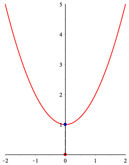
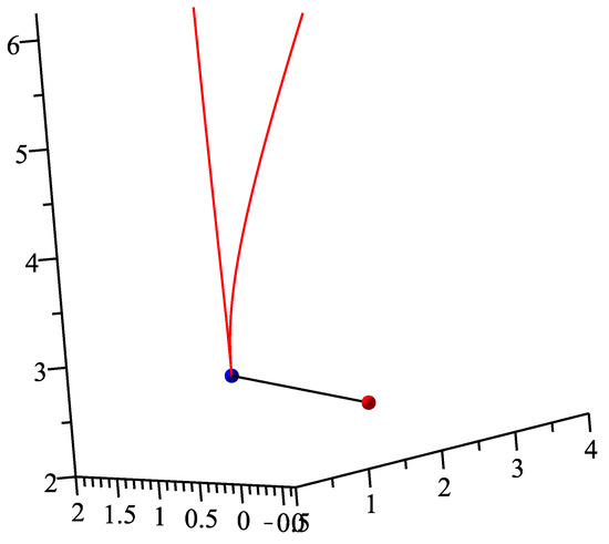
There are a parametric curve $c\left(t\right)=(t,1+t^2)$ and a test point $p=(0,0)$. The projection point and parametric value of the test point p are $(0,1)$ and $\alpha =0$, respectively. As to many initial values, the H-H-H method fails to converge to α. When the initial values are t = $-3,-2,-1.5,1.5,2,3,$ respectively, there repeatedly appear alternating oscillatory iteration values of 0.412415429665, −0.412415429665. Furthermore, for a parametric curve $c\left(t\right)=(t,1+a_1{t}^2+a_2{t}^4+a_3{t}^6+a_4{t}^8+a_5{t}^{10})$, $a_1\ne 0,a_2\ne 0,a_3\ne 0,a_4\ne 0,a_5\ne 0$, about $p=(0,0)$ and many initial values, the H-H-H method fails to converge to α (see Figure 2).

Figure 2. Geometric illustration for counterexample 1.

Counterexample 2.

There are a parametric curve $c\left(t\right)=(t,t^2,t^4,t^6,1+t^2+t^4+t^6+t^8)$ and a test point $p=(0,0,0,0,0)$. The projection point and parametric value of the test point p are $(0,0,0,0,1)$ and α = 0, respectively. For any initial value, the H-H-H method fails to converge to α. When the initial values are $t=-5,-4,-3,-2,-1,1,2,3,4,5,$ respectively, there repeatedly appear alternating oscillatory iteration values of 0.304949569175, −0.304949569175. Furthermore, for a parametric curve $c\left(t\right)=(a_{0}t$, $a_1{t}^2$, $a_2{t}^4$, $a_3{t}^6$, $1+a_4{t}^2+a_5{t}^4+a_6{t}^6+a_7{t}^8+a_8{t}^{10}+a_9{t}^{28})$, $a_0\ne 0,a_1\ne 0,a_2\ne 0,a_3\ne 0,a_4\ne 0,a_5\ne 0,a_6\ne 0,a_7\ne 0,a_8\ne 0,a_9\ne 0$, about point $p=(0,0,0,0,0)$ and any initial value, the H-H-H method fails to converge to α.

Counterexample 3.

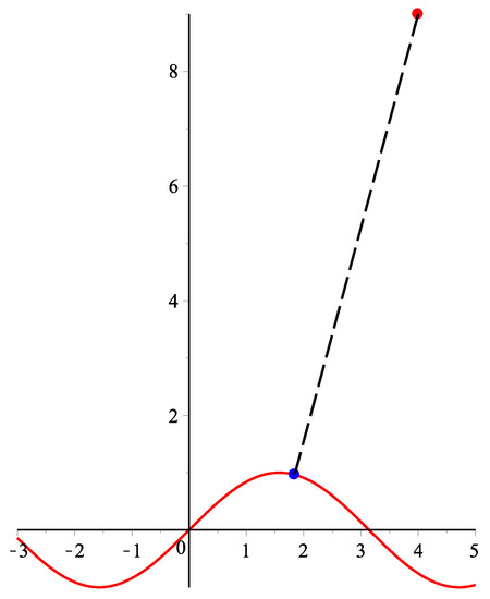
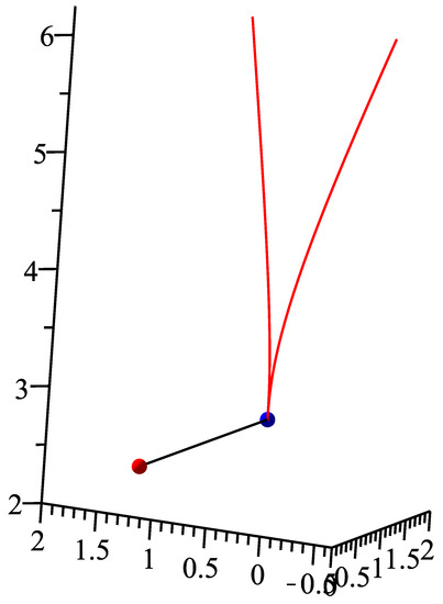
There are a parametric curve $c\left(t\right)=(t,sin(t\left)\right),t\in [0,3]$ and a test point $p=(4,9)$. The projection point and parametric value of the test point p are $(1.842576,0.9632946)$ and $\alpha =1.842576$, respectively. For point p and any initial value, the H-H-H method fails to converge to α. When the initial values are $t=-5,-4,-3,-2,-1,1,2,3,4,5,$ respectively, there repeatedly appear alternating oscillatory iteration values of 2.165320, 0.0778704, 6.505971, 9.609789. In addition, for a parametric curve $c\left(t\right)=(t,sin(at\left)\right)$, $a\ne 0$, for any test point p and any initial value, the H-H-H method fails to converge to α (see Figure 3).

Figure 3. Geometric illustration of counterexample 3.

Counterexample 4.

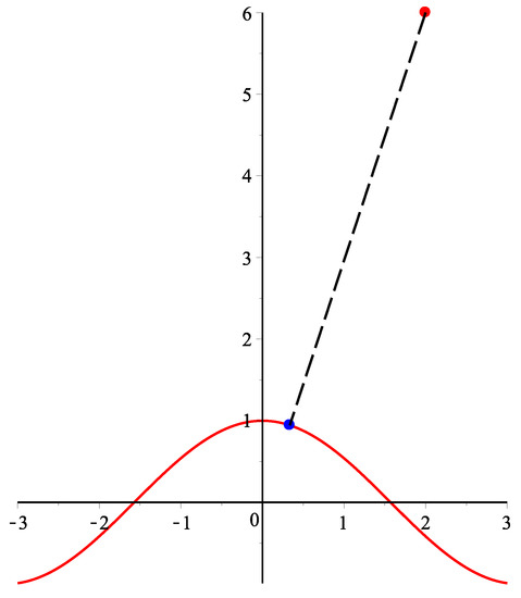
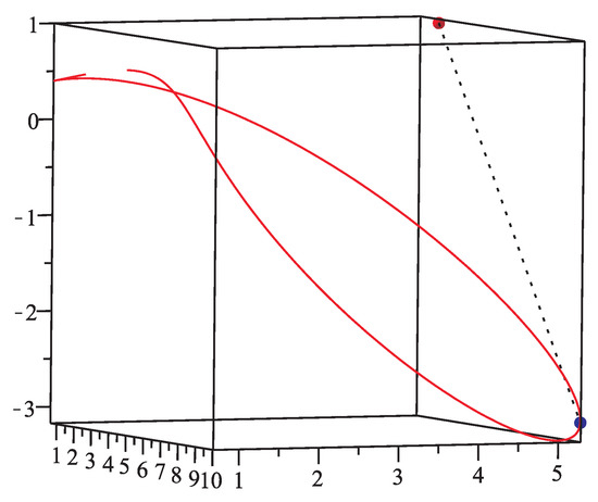
There are a parametric curve $c\left(t\right)=(t,cos(t\left)\right),t\in [0,3]$ and a test point $p=(2,6)$. The projection point and parametric value of the test point p are $(0.3354892$, $0.9442493)$ and $\alpha =0.3354892$, respectively. For test point p and any initial value, the H-H-H method fails to converge to α. When the initial value is $t=-5$, alternating oscillatory iteration values of 5.18741299662, 3.59425803253, −0.507188248308, 1.6901041247, 3.82746208506 repeatedly appear. When the initial value is t = 2, very irregular oscillatory iteration values of 0.652526561595, −0.720371663877, −2.39555359952, 0.365881194752, 2.06880954777, 3.18725085474, 1.71447110647, etc. appear In addition, for a parametric curve $c\left(t\right)=(t,cos(at\left)\right)$, $a\ne 0$, for any test point p and any initial value, the H-H-H method fails to converge to α (see Figure 4).

Figure 4. Geometric illustration of counterexample 4.

Counterexample 5.

There are a parametric curve $c\left(t\right)=(t,t,t,t,sin(t\left)\right),t\in [6,9]$ and a test point $p=(3,5,7,9,11)$. The projection point and parametric value of the test point p are (7.310786, 7.310786, 7.310786, 7.310786, 0.8560612) and $\alpha =7.310786$, respectively. For point p and any initial value, the H-H-H method fails to converge to α. When the initial values are $t=-9,-7,-5,6,8,$ respectively, there repeatedly appear alternating oscillatory iteration values of 7.24999006346, 6.37363460615. In addition, for a parametric curve $c\left(t\right)=(t,t,t,t,sin(at\left)\right),t\in [6,9]$, $a\ne 0$ with a test point $p=(3,5,7,9,11)$, for any initial value, the H-H-H method fails to converge to α.

Counterexample 6.

There are a parametric curve $c\left(t\right)=(t,t,t,t,cos(t\left)\right),t\in [4,8]$ and a test point $p=(2,4,6,8,10)$. The projection point and parametric value of the test point p are (5.883406, 5.883406, 5.883406, 5.883406, 0.9211469) and $\alpha =5.883406$, respectively. For point p and any initial value, the H-H-H method fails to converge to α. When the initial values are $t=,-4,-3,-2,4,5,6,7,$ respectively, there repeatedly appear alternating oscillatory iteration values of 4.17182145828, 7.80116702003. In addition, about a parametric curve $c\left(t\right)=(t,t,t,t,cos(at\left)\right),t\in [4,8]$, $a\ne 0$ with a point $p=(2,4,6,8,10)$, for any initial value, the H-H-H method fails to converge. The non-convergence explanation of the three counterexamples below are similar to the preceding six ones and omitted to save space.

Counterexample 7.

There are a parametric curve $c\left(t\right)=(t^4+2t^2+1$, $t^2+1$, $t^4+2$, $t^2$, $3t^6+t^4+2t^2)$ in five-dimensional Euclidean space and a test point $p=(0,0,0,0,0)$. The projection point and parametric value of the test point p are $(1,1,2,0,0)$ and $\alpha =0$, respectively. For any initial value $t_0$, the H-H-H method fails to converge. We also test many other examples, such as when parametric curve is completely symmetrical and the point is on the symmetrical axis of parametric curve. For any initial value $t_0$, the same results remain.

Counterexample 8.

There are a parametric curve $c\left(t\right)=(t$,sin$\left(t\right),t$,sin$\left(t\right),$sin$\left(t\right))$, $t\in [-5,5]$ in five-dimensional Euclidean space and a test point $p=(3,4,5,6,7)$. The corresponding orthogonal projection parametric value α are −3.493548, −2.280571, 1.875969, 4.791677, respectively. For any initial value $t_0$, the H-H-H method fails to converge.

Counterexample 9.

There is a parametric curve $c\left(t\right)=$(sin$(t$),cos$\left(t\right),t,$ sin$\left(t\right)$,cos$\left(t\right))$, $t\in [-5,5]$ in five-dimensional Euclidean space and a test point $p=(3,4,5,6,7)$. The corresponding orthogonal projection parametric value α are −4.833375, −3.058735, 0.9730030, 3.738442, respectively. For any initial value $t_0$, the H-H-H method fails to converge.

3.2. The Improved Algorithm

Due to the H-H-H method’s non-convergence for some special cases, the improved algorithm is presented to ensure the converge for any parametric curve, test point and initial value. The most classic Newton’s method can be expressed as

$$t_{m+1}=t_m-\frac{f\left(t_m\right)}{f^{\prime }\left(t_m\right)},$$

(16)

where $f\left(t\right)=<T_1,V_1>=0$, $T_1=c^{\prime }\left(t\right),V_1=p-c\left(t\right)$. It converges faster than the H-H-H method. However, the convergence of this depends on the chosen initial value. Only when the local convergence condition for the Newton’s method is satisfied, the method can acquire high effectiveness. In order to improve the robustness and rate of convergence, based on the the H-H-H method, our method is proposed. Combining the respective advantage of their two methods, if the iterative parametric value of the H-H-H method is satisfied with the convergence condition of the Newton’s method, we then go to the method to increase the convergence process. Otherwise, we continue the H-H-H method until it can generate iterative parametric value while satisfying the convergence condition by the Newton’s method, and we then go to the iterative process mentioned above. Thus, we run to the end of the whole process. The procedure not only ensures the robustness of convergence, but also improves the convergence rate. Using a hybrid strategy, our method is faster than current methods and independent from the initial value. Some numerical examples verify our conclusion. Our method can be realized as follows (see Figure 5).

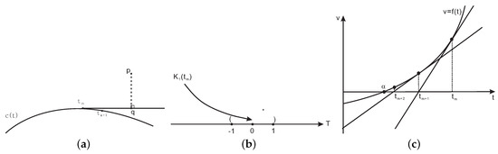
Figure 5. Geometric illustration for our method. (a) Running the H-H-H method; (b) Judging the H-H-H method whether being satisfied the convergence condition of fixed point theorem for the Newton’s iterative method; (c) Running the Newton’s iterative method.

Hybrid second order method

Input: Initial iterative value $t_0$, test point p and parametric curve $c\left(t\right)$ in an n-dimensional Euclidean space.

Output: The corresponding parameter $\alpha$ determined by orthogonal projection point.

Step 1. 

Initial iterative parametric value $t_0$ is input.

Step 2. 

Using the iterative Equation (3), calculate the parametric value $K_1\left(t_0\right)$, and update $K_1\left(t_0\right)$ to $t_1$, namely, $t_1=K_1\left(t_0\right)$.

Step 3. 

Determine whether absolute value of difference between the current $t_0$ and the new $t_1$ is near 0. If so, this algorithm is ended.

Step 4. 

Substitute the new $t_1$ into $\left|\frac{f\left(t\right)f^{″}\left(t\right)}{f^{\prime }{\left(t\right)}^2}\right|$, determine if $\left|\frac{f\left(t_1\right)f^{″}\left(t_1\right)}{f^{\prime }{\left(t_1\right)}^2}\right|<1$.

If ($\left|\frac{f\left(t_1\right)f^{″}\left(t_1\right)}{f^{\prime }{\left(t_1\right)}^2}\right|<1)$ {

Using Newton’s iterative Equation (16), compute $t_0=t_1-\frac{f\left(t_1\right)}{f^{\prime }\left(t_1\right)}$ until absolute value of difference between the current $t_1$ and the new $t_0$ is near 0; then, this algorithm ends.

}

Else {

  turn to Step 2.

}

Remark 1.

Firstly, a geometric illustration of our method in Figure 5 would be presented. Figure 5a illustrates the second step of our method where the next iterative parameter value $t_{m+1}=K_1\left(t_m\right)=t_m+\frac{⟨c^{\prime }\left(t_m\right),p-c\left(t_m\right)⟩}{⟨c^{\prime }\left(t_m\right),c^{\prime }\left(t_m\right)⟩}$ is determined by the iterative Equation (3). During the iterative process, the step $\mathsf{\Delta }t$ will become smaller and smaller. Thus, the next iterative parameter value $t_{m+1}$ comes close to parameter value $t_m$ but far from the footpoint q. If the third step of our method is not over, then our method goes into the fourth step. Figure 5b is judging condition of a fixed point theorem of the fourth step of our method. If $T=\left|\frac{f\left(t\right)f^{″}\left(t\right)}{f^{\prime }{\left(t\right)}^2}\right|<1$, then it turns to the Newton’s method in Figure 5c until it runs to the end of the whole process of Newton’s second order iteration; otherwise, it goes to the second step in Figure 5a.

Secondly, we give an interpretation for the singularity case of the iterative Equation (16). As to some special cases where the H-H-H method is not convergent in Section 3.1, our method still converges. We test many examples for arbitrary initial value, arbitrary test point and arbitrary parametric curve and find that our method remains more robust to converge than the H-H-H method. If the first order derivative $f^{\prime }\left(t_m\right)$ of the iterative Equation (16) develops into 0, i.e., $f^{\prime }\left(t_m\right)=0$ about some non-negative integer m, we use a perturbed method to solve the special problem, which adopts the idea in [23,45]. Namely, the function $f^{\prime }\left(t_m\right)=0$ could be increased by a very small positive number ε, i.e., $f^{\prime }\left(t_m\right)=f^{\prime }\left(t_m\right)+\epsilon$, and then the iteration by Equation (16) is continued in order to calculate the parameter value. On the other hand, if the curve can be parametrized by a (piece-wise) polynomial, then the fast root-finding schemes such as Bézier clipping [28,29] are efficient ones. The only issue is the $C^1$ discontinuities that can be checked in a post-process. One then does not need any initial guess on the parameter value.

Thirdly, if the curve is only $C^0$ continuous, and the closest point can be exactly such a point, then the derivative is not well defined and our method may fail to find such a point. Namely, there are singular points on the parametric curve. We adopt the following technique to solve the problem of singularity. We use the methods [46,47,48] to find all singular points on the parametric curve and the corresponding parametric value of each singular point as many as possible. Then, the hybrid second order method comes into work. If the current iterative parametric value $t_m$ is the corresponding parametric value of a singular point, we make a very small perturbation ε to the current iterative parametric value $t_m$, i.e., $t_m=t_m+\epsilon$. The purpose of this behavior is to enable the hybrid second order method to run normally. Then, from all candidate points (singular points and orthogonal projection points), a corresponding point is selected so that the distance between the corresponding point and the test point is the minimum one. When the entire program terminates, the minimum distance and its corresponding parameter value are found.

3.3. Convergence Analysis of the Improved Algorithm

In this subsection, we prove the convergence analysis of our method.

Theorem 2.

In Reference [49] (Fixed Point Theorem)

If $\varphi \left(x\right)\in C[c,d]$, $\varphi \left(x\right)\in [c,d]$ for all $x\in [c,d]$; furthermore, if ${\varphi }^{\prime }\left(x\right)$ exists on $(c,d)$ and a positive constant $L<1$ exists with $\left|{\varphi }^{\prime }\left(x\right)\right|\le L$ for all $x\in (c,d)$, then there exists exactly one fixed point in $[c,d]$.

In addition, if ${\displaystyle \varphi \left(t\right)=t-\frac{f\left(t\right)}{f^{\prime }\left(t\right)}}$, the corresponding fixed point theorem of Newton’s method is as follows:

Theorem 3.

Let $f:\left[c,d\right]\to \left[c,d\right]$ be a differentiable function, if for all $t\in \left[c,d\right]$, there is

$$\left|\frac{f\left(t\right)f^{″}\left(t\right)}{f^{\prime 2}\left(t\right)}\right|<1.$$

(17)

Then, there is a fixed point $l_0\in \left[c,d\right]$ in Newton’s iteration expression (16) such that ${\displaystyle l_0=l_0-\frac{f\left(l_0\right)}{f^{\prime }\left(l_0\right)}}$. Meanwhile, the iteration sequence $\left\{t_m\right\}$ been from expression (16) can converge to the fixed point when $\forall t_0\in \left[c,d\right]$.

Theorem 4.

Our method is second order convergent.

Proof: 

Let $\alpha$ be a simple zero for a nonlinear function $f\left(t\right)=<T_1,V_1>=0$, where $T_1=c^{\prime }\left(t\right),V_1=p-c\left(t\right)$. Using Taylor’s expansion, we have

$$f\left(t_m\right)=f^{\prime }\left(\alpha \right)[e_m+b_2{e}_m^2+b_3{e}_m^3+o\left(e_m^4\right)],$$

(18)

$$f^{\prime }\left(t_m\right)=f^{\prime }\left(\alpha \right)[2b_2{e}_m+3b_3{e}_m^2+o\left(e_m^3\right)],$$

(19)

where ${\displaystyle b_k=\frac{f^{\left(k\right)}\left(\alpha \right)}{k!f^{\prime }\left(\alpha \right)},k=2,3,\dots }$, and $e_m=t_m-\alpha$. Combining with (15), we then have

$$y_m=\varphi \left(t_m\right)=t_m-\frac{f\left(t_m\right)}{f^{\prime }\left(t_m\right)}=\alpha +b_2{C}_0^2{e}_m^2+o\left(e_m^3\right).$$

(20)

This means that the convergence order of our method is 2. The proof is completed. □

Theorem 5.

Convergence of our method does not depend on the initial value.

Proof. 

According to the description of our method, if the iterative parametric value of the H-H-H method is satisfied with the convergence condition of the Newton’s method, we then go to the Newton’s method. Otherwise, we steadily adopt the H-H-H method until its iterative parametric value is satisfied with the convergence condition of the Newton’s method, and we go to Newton’s method. Then, we run to the end of the whole process. Theorem 1 ensures that it does not depend on the initial value. If our method goes to the fourth step and if it is appropriate to the condition of the fixed point theorem (Theorem 3), Newton’s method is realized by our method. Then, the fourth step of our method being also independent of the initial value can be confirmed by Theorem 3. In brief, convergence of our method does not depend on the initial value via the whole algorithm execution process. The proof is completed. □

4. Numerical Experiments

In order to illustrate the superiority of our method to other algorithms, we provide five numerical examples to confirm its robustness and high efficiency. From Table 1, Table 2, Table 3, Table 4, Table 5, Table 6, Table 7, Table 8, Table 9, Table 10, Table 11, Table 12, Table 13 and Table 14, the iterative termination criteria is satisfied such that $\left|t_m-\alpha \right|<{10}^{-17}and\left|t_{m+1}-t_n\right|<{10}^{-17}$. All numerical results were computed through g++ in a Fedora Linux 8 environment. The approximate zero $\alpha$ reached up to the 17th decimal place is reflected. These results of our five examples are obtained from computer hardware configuration with T2080 1.73 GHz CPU and 2.5 GB memory.

Table 1. Running time for different initial values of Example 1 by our method with test point p = (2.0, 4.0, 2.0).

${\mathit{t}}_0$	0	2	4	5	6	8	9	10
$\alpha$	0.0	0.0	0.0	0.0	0.0	0.0	0.0	0.0
1	498,454	75,487	105,563	116,470	123,031	134,941	154,253	156,872
2	555,709	81,629	108,064	117,762	125,946	140,940	153,468	155,830
3	509,173	82,824	100,744	111,206	134,367	141,705	150,013	158,715
4	564,222	77,465	96,721	114,757	129,128	173,027	150,320	158,580
5	502,986	81,028	97,142	118,535	120,668	132,856	155,335	149,437
6	553,198	79,520	104,307	120,795	129,351	150,085	151,073	143,065
7	576,814	74,268	100,231	115,002	132,322	139,919	154,754	159,014
8	524,848	81,982	99,604	115,263	122,401	139,345	143,568	175,169
9	528,848	71,228	103,186	140,023	122,040	135,006	145,434	154,016
10	547,161	70,789	99,247	121,834	125,766	136,103	149,790	153,435
Average	536,142	77,622	101,481	119,165	126,502	142,393	150,801	156,413
Total Average	176,315

Table 2. Running time for different initial values of Example 1 by our method with test point p = (2.0, 2.0, 2.0).

${\mathit{t}}_0$	0	2	4	5	6	8	9	10
$\alpha$	0.0	0.0	0.0	0.0	0.0	0.0	0.0	0.0
1	595,515	92,371	119,904	135,660	148,751	162,758	171,535	177,355
2	648,825	91,746	119,348	135,284	148,531	162,541	171,333	176,431
3	595,772	91,633	119,248	135,322	148,222	162,240	171,095	176,501
4	648,472	91,565	119,139	135,355	148,165	191,884	171,366	176,395
5	595,856	91,556	119,168	135,406	148,144	162,224	171,417	176,507
6	648,305	91,532	119,018	135,316	148,169	183,342	171,413	176,473
7	647,406	91,587	119,069	135,283	148,197	162,291	171,282	176,397
8	595,423	91,617	119,247	135,140	14,8101	162,116	171,342	196,529
9	646,551	83,167	119,135	172,412	148,149	162,148	171,313	176,390
10	657,838	83,147	119,131	135,179	148,259	162,094	171,609	176,557
Average	627,996	89,992	119,241	139,036	148,269	167,364	171,371	178,554
Total Average	205,228

Table 3. Running time for different initial values of Example 2 by our method with test point p = (1.0, 3.0, 5.0).

${\mathit{t}}_0$	−2.4	−2.1	−2	−1.8	−1.6	−1.2	−1	−0.8
$\alpha$	−1.4118	0.61917	−1.4118	0.61917	−0.059	−0.059	1.84934	1.84934
1	88,695	90,501	75,137	68,499	52,014	24,731	26,295	28,444
2	89,958	91,254	79,411	64,563	54,321	22,014	26,278	28,024
3	83,956	95,063	79,553	63,237	54,683	22,733	24,813	28,760
4	83,623	96,033	82,022	68,075	51,098	23,270	24,573	26,707
5	83,368	95,700	76,197	63,518	51,752	22,321	24,644	26,586
6	83,631	97,303	80,984	62,608	53,473	21,658	24,009	28,209
7	87,286	94,655	78,483	66,844	52,277	23,502	25,554	28,725
8	87,150	96,316	79,215	64,333	51,554	23,217	26,234	28,295
9	86,300	89,399	94,487	66,665	50,279	23,190	25,791	26,160
10	89,761	96,377	82,362	64,371	50,367	22,332	23,929	27,273
Average	85,344	93,936	79,424	62,643	54,482	22,982	25,654	26,868
Total Average	56,417

Table 4. Running time for different initial values of Example 2 by our method with test point p = (2.0, 4.0, 8.0).

${\mathit{t}}_0$	−2.4	−−2.1	−−2	−1.8	−1.6	−1.2	−1	−0.8
$\alpha$	−0.6272	−0.1459	−0.6272	−1.2589	−0.1459	1.858	−1.2589	1.858
1	101,366	109,667	92,799	77,983	62,865	29,460	29,755	32,649
2	102,027	108,844	92,709	77,477	62,269	27,177	29,555	32,458
3	101,526	109,010	92,709	77,587	62,284	26,885	29,619	32,538
4	101,266	108,909	92,724	77,441	62,374	26,785	29,557	32,478
5	101,346	108,944	92,714	77,386	62,214	26,691	29,559	32,505
6	101,315	108,990	92,764	77,557	62,334	26,731	29,564	32,497
7	101,415	108,834	92,614	77,582	62,415	26,720	29,573	32,512
8	101,306	108,945	92,528	77,461	62,309	26,715	29,548	32,493
9	101,562	108,954	116,107	77,542	62,284	26,684	29,549	32,429
10	101,235	108,910	92,939	77,616	62,314	26,690	29,595	32,451
Average	101,436	109,001	95,061	77,563	62,366	27,054	29,587	32,501
Total Average	66,821

Table 5. Running time for different initial values of Example 2 by the algorithm [26].

${\mathit{t}}_0$	−2.4	−2.1	−2.0	−1.8	−1.6	−1.2	−1.0	−0.8
$\alpha$	−0.6272	−0.1459	−0.6272	−1.2589	−0.1459	1.858	−1.2589	1.858
1	633,173	660,734	566,675	470,236	391,687	171,352	175,965	198,543
2	597,065	628,741	565,012	485,368	367,539	161,649	185,457	197,798
3	652,494	675,268	600,951	463,899	396,359	163,879	188,682	187,128
4	649,281	653,066	573,597	460,967	385,325	156,876	182,979	195,214
5	622,109	687,282	568,766	472,217	402,669	170,876	189,508	202,540
6	633,737	627,667	562,864	490,735	374,340	165,445	175,457	191,037
7	584,705	637,608	563,523	468,230	395,411	163,631	175,676	187,539
8	607,439	693,001	585,948	449,706	400,728	161,467	189,216	187,433
9	637,036	639,359	671,613	444,834	359,918	157,235	188,119	195,867
10	580,678	640,082	587,577	472,368	369,954	159,834	181,510	207,033
Average	619,772	654,281	584,653	467,856	384,393	163,225	183,257	195,013
Total Average	406,556

Table 6. Running time for different initial values of Example 3 by our method with test point p = (3, 4, 5, 6, 7).

${\mathit{t}}_0$	−10	−8	−6	−4	4	8	12	16
$\alpha$	1.15874	1.15874	1.15874	1.15874	1.15874	1.15874	1.15874	1.15874
1	407,427	425,388	387,337	306,115	110,887	161,079	187,144	184,119
2	417,729	446,171	398,801	341,895	121,148	169,115	169,954	194,671
3	420,894	390,507	383,308	260,183	115,033	165,103	171,989	198,884
4	383,836	421,365	427,391	242,641	109,521	161,121	179,152	195,714
5	373,696	421,551	373,171	266,584	120,844	187,930	179,184	186,309
6	374,791	445,114	373,974	242,889	119,449	183,082	180,269	201,487
7	381,353	408,011	402,073	216,762	109,054	162,402	172,013	188,206
8	398,662	442,008	373,328	194,821	119,236	192,990	180,472	197,299
9	364,491	417,139	396,843	230,070	110,243	164,273	204,410	196,163
10	387,246	427,188	394,694	191,799	120,759	155,029	170,059	226,270
Average	391,013	424,444	391,092	249,376	115,617	170,212	179,465	196,912
Total Average	264,766

Table 7. Running time for different initial values of Example 3 by our method with test point p = (30, 40, 50, 60, 70).

${\mathit{t}}_0$	−10	−8	−6	−4	4	8	12	16
$\alpha$	1.235289	1.235289	1.235289	1.235289	1.235289	1.235289	1.235289	1.235289
1	1,190,730	475,499	453,879	369,551	133,651	191,093	208,202	223,695
2	1,031,760	500,975	486,534	380,881	133,638	190,959	208,490	236,637
3	482,018	475,395	450,480	297,272	133,674	199,528	208,292	223,312
4	428,081	475,588	475,100	277,356	133,635	186,919	208,438	223,802
5	455,282	475,033	448,776	296,510	133,535	220,570	208,139	223,471
6	428,321	499,776	448,617	277,353	133,590	220,625	208,046	223,213
7	428,246	474,978	474,667	247,245	133,620	192,326	208,101	230,791
8	453,374	502,500	448,503	235,415	133,594	220,635	208,087	223,183
9	426,949	474,816	474,167	275,526	133,546	198,204	245,226	223,213
10	452,306	499,605	448,409	235,207	134,128	173,843	208,127	262,661
Average	577,707	485,417	460,913	289,232	133,661	199,470	211,915	229,398
Total Average	323,464

Table 8. Running time for different initial values of Example 4 by our method.

${\mathit{t}}_0$	−100	−4	5	7	8	10	11	100
$\alpha$	1.106305	1.106305	1.106305	1.106305	1.106305	1.106305	1.106305	1.106305
1	63,345	35,580	27,069	41,551	22,304	36,858	21,478	72,257
2	63,192	36,203	28,160	41,733	20,042	38,680	20,338	71,620
3	61,306	33,833	27,400	44,198	23,078	37,704	23,757	73,108
4	66,627	34,502	26,014	44,160	21,147	39,374	22,530	70,154
5	62,583	35,053	29,275	42,800	20,817	39,339	23,046	73,189
6	63,957	34,398	25,650	42,282	22,184	37,376	20,070	75,872
7	60,865	35,929	28,944	42,134	19,964	40,078	21,943	71,608
8	63,522	35,427	27,578	41,688	23,650	39,456	21,076	76,283
9	60,551	35,508	28,563	44,542	20,280	38,463	20,596	71,781
10	62,216	33,987	27,830	46,130	22,781	39,209	20,349	73,296
Average	62,816	35,042	27,648	43,122	21,625	38,654	21,518	72,917
Total Average	40,418

Table 9. Running time for different initial values of Example 4 by the H-H-H method.

${\mathit{t}}_0$	−100	−4	5	7	8	10	11	100
$\alpha$	1.106305	1.106305	1.106305	1.106305	1.106305	1.106305	1.106305	1.106305
1	424,579	357,276	443,858	179,583	176,984	175,859	175,249	178,445
2	425,680	358,510	179,137	177,849	182,701	176,665	176,463	207,164
3	359,794	356,912	180,000	180,472	177,867	179,743	178,929	179,372
4	371,119	357,214	179,567	179,804	184,542	177,675	177,854	179,651
5	358,128	358,119	232,337	179,285	179,113	175,632	177,690	181,976
6	358,470	357,893	179,985	179,941	178,600	178,289	178,565	181,868
7	358,083	359,391	178,815	177,857	177,613	178,014	177,385	179,361
8	477,393	357,011	178,029	179,525	175,684	176,000	175,413	180,966
9	356,254	359,356	176,148	178,581	176,351	177,024	185,103	180,013
10	356,801	359,773	213,327	177,252	176,993	178,060	177,655	181,427
Average	384,630	358,146	214,120	179,015	178,645	177,296	178,031	183,024
Total Average	231,613

Table 10. Running time for different initial values of Example 4 by the Algorithm [6].

${\mathit{t}}_0$	−100	−4	5	7	8	10	11	100
$\alpha$	1.106305	1.106305	1.106305	1.106305	1.106305	1.106305	1.106305	1.106305
1	681,353	107,102	119,083	120,328	122,504	115,181	113,566	542,116
2	725,571	124,514	136,810	121,111	116,824	111,116	117,466	5,250,481
3	669,249	111,052	122,151	125,261	124,865	116,105	120,309	5,523,805
4	713,982	112,146	131,494	118,104	121,099	111,410	118,658	5,407,166
5	699,433	111,347	118,830	121,003	118,694	115,182	124,917	5,259,412
6	693,396	113,323	116,046	109,176	108,194	111,420	117,342	5,508,049
7	691,375	114,667	115,748	123,330	127,812	118,635	119,208	5,348,517
8	663,125	107,484	127,493	120,134	116,818	111,717	117,079	5,446,703
9	731,148	128,918	122,897	120,947	120,985	113,777	125,463	5,251,580
10	676,286	128,567	130,775	118,031	116,725	111,095	108,275	5,356,125
Average	694,492	115,912	124,133	119,743	119,452	113,564	118,228	5,377,300
Total Average	847,853

Table 11. Running time for different initial values of Example 5 by our method.

${\mathit{t}}_0$	−100	−4	5	7	8	10	11	100
$\alpha$	1.28902	1.28902	1.28902	1.28902	1.28902	1.28902	1.28902	1.28902
1	52,010	27,426	21,791	33,323	18,399	29,551	16,486	58,995
2	50,335	29,269	23,949	32,810	15,820	30,342	16,066	58,080
3	49,047	26,841	23,061	37,063	19,611	31,569	19,756	57,458
4	52,651	29,124	21,403	33,838	17,472	33,295	18,583	54,566
5	49,871	29,814	25,062	35,870	16,655	32,949	18,304	61,860
6	53,651	28,678	19,550	35,731	18,373	31,429	16,342	59,570
7	47,275	28,115	24,177	35,456	16,933	30,510	18,010	59,042
8	49,982	27,896	22,639	34,292	19,927	30,959	16,449	63,652
9	49,704	29,359	22,502	34,164	17,274	30,391	16,044	61,373
10	51,268	25,859	22,736	37,190	17,342	30,864	16,060	56,564
Average	50,579	28,238	22,687	34,974	17,781	31,186	17,210	59,116
Total Average	32,721

Table 12. Running time for different initial values of Example 5 by the Algorithm [6].

${\mathit{t}}_0$	−100	−4	5	7	8	10	11	100
$\alpha$	1.28902	1.28902	1.28902	1.28902	1.28902	1.28902	1.28902	1.28902
1	308,942	191,002	152,199	235,287	114,568	199,404	110,512	379,771
2	348,554	175,800	146,728	232,260	102,698	190,860	101,754	352,834
3	311,680	190,863	148,384	242,131	118,602	207,376	125,517	408,978
4	332,421	166,849	145,131	234,536	102,795	198,956	113,523	370,826
5	319,660	185,059	160,358	235,072	108,557	211,429	119,911	350,188
6	329,882	177,252	132,242	233,702	120,945	199,978	107,366	363,299
7	304,977	200,038	151,398	229,166	102,315	220,162	122,013	354,466
8	326,645	171,624	137,588	228,181	113,627	195,782	108,512	369,899
9	291,369	191,878	156,871	247,614	108,418	189,534	112,319	363,905
10	326,221	174,148	139,415	239,836	128,377	190,831	111,411	378,781
Average	320,035	182,451	147,031	235,779	112,090	200,431	113,284	369,294
Total Average	210,049

Table 13. Comparison of iterations by different methods in Example 5.

${\mathit{t}}_0$	$-100.0$	$-4.0$	$5.0$	$7.0$	$8.0$	$10.0$	$11.0$	$100.0$
$\alpha$	1.28902	1.28902	1.28902	1.28902	1.28902	1.28902	1.28902	1.28902
H-H-H method [38,39,40]	NC	NC	NC	NC	NC	NC	NC	NC
Second order method [6]	75	30	32	32	33	29	31	101
Newton’s method	NC	NC	NC	NC	NC	NC	NC	NC
Our method	15	19	17	17	15	17	15	23

Table 14. Time comparison of various algorithms.

Algorithms	Ours	H-H-H	Algorithm [1]	Algorithm [14]	Algorithm [6]	Algorithm [26]
Time ($\mathsf{\mu }$s)	145.5	231.6	680.8	1270.8	528.9	406.6

Example 1.

There is a parametric curve $c\left(t\right)=(f_1\left(t\right),f_2\left(t\right),f_3\left(t\right))=(6t^7+t^5,5t^8+3t^6,10t^{12}+8t^8+6t^6+4t^4+2t^2+3),t\in [-2,2]$ in three-dimensional Euclidean space and a test point $p=(p_1,p_2,p_3)=(2.0,4.0,2.0)$. Using our method, the corresponding orthogonal projection parametric value is $\alpha =0.0$, the initial values $t_0$ are 0,2,4,5,6,8,9,10, respectively. For each initial value, the iteration process runs 10 times and then 10 different iteration times in nanoseconds, respectively. In Table 1, the average run time of our method for eight different initial values are 536,142, 77,622, 101,481, 119,165, 126,502, 142,393, 150,801, 156,413 nanoseconds, respectively. Finally, the overall average running time is 176,315 nanoseconds (see Figure 6). If test point p is (2.0, 2.0, 2.0), the corresponding orthogonal projection parametric value is $\alpha =0.0$, we replicate the procedure using our method and report the results in Table 2. In Table 2, the average running time of our method for 8 different initial values are 627,996, 89,992, 119,241, 139,036, 148,269, 167,364, 167,364, 178,554 nanoseconds, respectively. Finally, the overall average running time is 205,228 nanoseconds (see Figure 7). However, for the above two cases, the H-H-H method does not converge for any initial iterative value.

Figure 6. Geometric illustration for the test point p = (2.0, 4.0, 2.0) of Example 1.

Figure 7. Geometric illustration for the test point p = (2.0, 2.0, 2.0) of Example 1.

Because of a singular point on the parametric curve, we have also added some pre-processing steps before our method. (1) Find the singular point (0,0,3) and the corresponding parametric value 0 by using the methods [21,46,47,48]. (2) Using our method, the orthogonal projection points of test points (2,4,2) and (2,2,2) and their corresponding parameter values 0 and 0 are calculated, respectively. (3) From all candidate points(singular point and orthogonal projection point), corresponding point is selected so that the distance between the corresponding point and the test point is the minimum one. In Figure 6, the blue point denotes singular point (0,0,3), which is also the orthogonal projecting point of the test point (2,4,2). This is the same for the blue point in Figure 7.

Example 2.

There is a spatial quartic quasi-rational Bézier curve ${\displaystyle c\left(t\right)=(f_1\left(t\right),f_2\left(t\right),f_3\left(t\right))=(\frac{u\left(t\right)}{a\left(t\right)},\frac{v\left(t\right)}{a\left(t\right)},\frac{w\left(t\right)}{a\left(t\right)})}$, where $u\left(t\right)=2t^4+3t^3+3t^2+12t+1$, $v\left(t\right)=4t^4+3t^3+7t^2+7t+21$, $w\left(t\right)=5t^4+t^3+9t^2+11t+13$, $a\left(t\right)=4t^4+8t^3+17t^2+15t+6,t\in [-2,2]$ and a test point $p=(p_1,p_2,p_3)=(1.0,3.0,5.0)$. The corresponding orthogonal projection parametric value α are $-1.4118250062741212$, $-0.61917136491841674$, $-0.059335038305820650$, $1.8493434997820080$, respectively. Using our method, the initial values $t_0$ are $-2.4$,$-2.1$,$-2.0$,$-1.8$,$-1.6$,$-1.2$,$-1.0$,$-0.8$, respectively. For each initial value, the iteration process runs 10 times and then 10 different iteration times in nanoseconds, respectively. From Table 3, the average running time of our method for eight different initial values are 85,344, 93,936, 79,424, 62,643, 54,482, 22,982, 25,654, 26,868 nanoseconds, respectively. Finally, the overall average running time is 56,417 nanoseconds (see Figure 8). If test point p is $(2.0,4.0,8.0)$, the corresponding orthogonal projection parametric value α are $-1.2589948653798823$, $-0.62724968160147096$,$-0.14597283439336865$, $1.8584532894110559$, respectively. We firstly replicate the procedure using our method and report the results in Table 4. From Table 4, the average running time of our method for eight different initial iterative values are 101,436, 109,001, 95,061, 77,563, 62,366, 27,054, 29,587, 32,501 nanoseconds, respectively. Finally, the overall average running time is 66,821 nanoseconds (see Figure 9). We then replicate the procedure using the algorithm [26] and report the results in Table 5. From Table 5, the average running time of the algorithm [26] for eight different initial values are 619,772, 654,281, 584,653, 467,856, 384,393, 163,225, 183,257, 195,013 nanoseconds, respectively. Finally, the overall average running time is 406,556 nanoseconds. However, for the above two cases, the H-H-H method does not converge for any initial value.

Figure 8. Geometric illustration for the first case of Example 2.

Figure 9. Geometric illustration for the second case of Example 2.

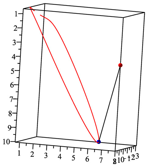
Example 3.

There is a parametric curve $c\left(t\right)=(f_1\left(t\right),f_2\left(t\right),f_3\left(t\right),f_4\left(t\right),f_5\left(t\right))=(cos\left(t\right),sin\left(t\right),t,cos\left(t\right),sin\left(t\right)),t\in [-2,2]$ in five-dimensional Euclidean space and a test point $p=(p_1,p_2,p_3,p_4,p_5)=(3.0,4.0,5.0,6.0,7.0)$. Using our method, the corresponding orthogonal projection parametric value is $\alpha =1.1587403612284800$, the initial values $t_0$ are $-10,-8,-6,-4,4,8,12,16,$ respectively. For each initial value, the iteration process runs 10 times and then 10 different iteration times in nanoseconds, respectively. In Table 6, the average running time of our method for eight different initial values are 391,013, 424,444, 391,092, 249,376, 115,617, 170,212, 179,465, 196,912 nanoseconds, respectively. Finally, the overall average running time is 264,766 nanoseconds. If test point p is $(30.0,40.0,50.0,60.0,70.0)$, the corresponding orthogonal projection parametric value α is $1.2352898417860202$. We then replicate the procedure using our method and report the results in Table 7. In Table 7, the average running time of our method for eight different initial values are $\mathrm{577,707}$, $\mathrm{485,417}$, $\mathrm{460,913}$, $\mathrm{289,232}$, $\mathrm{133,661}$, $\mathrm{199,470}$, $\mathrm{211,915}$, $\mathrm{229,398}$ nanoseconds, respectively. Finally, the overall average running time is 323,464 nanoseconds. However, for the above parametric curve and many test points, the H-H-H method does not converge for any initial value.

Example 4.

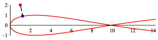
(Reference to [6])There is a parametric curve $c\left(t\right)=(f_1\left(t\right),f_2\left(t\right))=(t^2,sin\left(t\right)),t\in [-3,3]$ in two-dimensional Euclidean space and a test point $p=(p_1,p_2)=(1.0,2.0)$. The corresponding orthogonal projection parametric value is $\alpha =1.1063055095030472$. Using our method, the initial values $t_0$ are $-100,-4,5,7,8,10,11,100,$ respectively. For each initial value, the iteration process runs 10 times and then 10 different iteration times in nanoseconds, respectively. In Table 8, the average running time of our method for eight different initial iterative values are 62,816, 35,042, 27,648, 43,122, 21,625, 38,654, 21,518, 72,917 nanoseconds, respectively. Finally, the overall average running time is 40,418 nanoseconds (see Figure 10). Implementing the same procedure, the overall average running time given by the H-H-H method is 231,613 nanoseconds in Table 9, while the overall average running time given by the second order method [6] is 847,853 nanoseconds in Table 10. Thus, our method is faster than the H-H-H method [38,39,40] and the second order method [6].

Figure 10. Geometric illustration for Example 4.

Example 5.

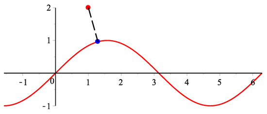
(Reference to [6])There is a parametric curve $c\left(t\right)=(f_1\left(t\right),f_2\left(t\right))=(t,sin\left(t\right)),t\in [-3,3]$ in two-dimensional Euclidean space and a test point $p=(p_1,p_2)=(1.0,2.0)$, the corresponding orthogonal projection parametric value is $\alpha =1.2890239979093887$. Using our method, the initial values $t_0$ are $-100,-4,5,7,8,10,11,100,$ respectively. For each initial value, the iteration process runs 10 times and then 10 different iteration time in nanoseconds, respectively. In Table 11, the average running time of our method for eight different initial values are $\mathrm{50,579}$, $\mathrm{28,238}$, $\mathrm{22,687}$, $\mathrm{34,974}$,$\mathrm{17,781}$, $\mathrm{31,186}$, $\mathrm{17,210}$, $\mathrm{59,116}$ nanoseconds, respectively. Finally, the overall average running time is 32,721 nanoseconds (see Figure 11). We then replicate the procedure using the second order method [6] and report the results in Table 12. In Table 12, the average running time of the second order method [6] for 8 different initial values are $\mathrm{320,035}$, $\mathrm{182,451}$, $\mathrm{147,031}$, $\mathrm{235,779}$, $\mathrm{112,090}$, $\mathrm{200,431}$, $\mathrm{113,284}$, $\mathrm{369,294}$ nanoseconds, respectively. Finally, the overall average running time is 210,049 nanoseconds. In addition, we compare the iterations by different methods where the NC denotes non-convergence in Table 13.

Figure 11. Geometric illustration for Example 5.

Remark 2.

From the results of five examples, the overall average running time of our method is 145.5 μs. From the results of Table 9, the overall average running time of the H-H-H method is 231.6 μs. From results of six examples in [26], the overall average running time of the algorithm [1] is 680.8 μs. From results of six examples in [26], the overall average running time of the algorithm [14] is 1270.8 μs. From results of Table 5, the overall average running time of the algorithm [26] is 406.6 μs. From results of Table 10 and Table 12, the overall average running time of the algorithm [6] is 528.9 μs. Table 14 displays time comparison for these algorithms. In short, the robustness and efficiency of our method are more superior to those of the existing algorithms [1,6,14,26,38,39,40].

Remark 3.

For general parametric curve containing the elementary functions, such as sin$\left(t\right)$, cos$\left(t\right)$, $e^t$, $lnt$, $arcsint$, $arccost$, etc., it is very difficult to transform general parametric curve into Bézier-type curve. In contrast, our method can deal with the general parametric curve containing the elementary functions. Furthermore, the convergence of our method does not depend on the initial value. From Table 13, only the H-H-H method or the Newton’s method can not ensure convergence, while our method can ensure convergence. For multiple solutions of orthogonal projection, our approach works as follows:

(1) 

The parameter interval $[a,b]$ of parametric curve $c\left(t\right)$ is divided into M identical subintervals.

(2) 

An initial value is selected randomly in each interval.

(3) 

Using our method and using each initial parametric value, do iterations, respectively. Suppose that the iterative parametric values are ${\alpha }_1$, ${\alpha }_2$, …, ${\alpha }_M$, respectively.

(4) 

Calculate the local minimum distances $d_1,d_2,\dots ,d_M$, where $d_i=∥p-c\left({\alpha }_i\right)∥$.

(5) 

Seek the global minimum distance $d=∥p-c\left(\alpha \right)∥$ from $\{∥p-c\left(a\right)∥,d_1,d_2,\dots ,d_M$, $∥p-c\left(b\right)∥\}$.

If we are to solve all solutions as far as possible, we urge the positive integer M to be as large as possible.

We use Example 2 to illustrate how the procedure works, where, for $t\in [-2,2]$, three parameter values are $-1.4118250062741212$, $-0.61917136491841674$, $1.8493434997820080$, respectively. It is easy to find that the projection point with the parameter value $-0.61917136491841674$ will be the one with minimum distance, whereas other projection points without these parameter values can not be the one with minimum distance. Thus, only the orthogonal projection point with minimum distance remains after the procedure to select multiple orthogonal projection points.

Remark 4.

We have done many test examples including five test examples. In the light of these test results, our method has good convergent properties for different initial values, namely, if initial value is $t_0$, then the corresponding orthogonal projection parametric value α for the orthogonal projection point of the test point p is suitable for one inequality relationship

$$\left|⟨p-c\left(\alpha \right),c^{\prime }\left(\alpha \right)⟩\right|<{10}^{-17}.$$

(21)

This indicates that the inequality relationship satisfies requirements of Equation (4). This shows that convergence of our method does not depend on the initial value. Furthermore, our method is robust and efficient, which is satisfied with the previous two of ten challenges proposed by [50].

5. Conclusions

This paper discusses the problem related to a point orthogonal projection onto a parametric curve in an n-dimensional Euclidean space on the basis of the H-H-H method, combining with a fixed point theorem of Newton’s method. Firstly, we run the H-H-H method. If the current iterative parametric value from the H-H-H method is satisfied with the convergence condition of the Newton’s method, we then go to the method to increase the convergence rate. Otherwise, we continue the H-H-H method to generate the iterative parametric value with satisfaction of the local convergence condition by the Newton’s method, and we then go to the previous step. Then, we run to the end of the whole process. The presented procedures ensure the convergence of our method and it does not depend on the initial value. Analysis of convergence demonstrates that our method is second order convergent. Some numerical examples confirm that our method is more efficient and performs better than other methods, such as the algorithms [1,6,14,26,38,39,40].

In this paper, our discussion focuses the algorithms in the parametric curve $C^2$. For the parametric curve being $C^0$,$C^1$, piecewise curve or having singular points, we only present a preliminary idea. However, we have not completely implemented an algorithm for this kind of spline with low continuity. In the future, we will try to construct several brand new algorithms to handle the kind of spline with low continuity such that they can ensure very good robustness and efficiency. In addition, we also try to extend this idea to handle point orthogonal projecting onto implicit curves and implicit surfaces that include singularity points. Of course, the realization of these ideas is of great challenge. However, it is of great value and significance in practical engineering applications.

References

- Ma, Y.L.; Hewitt, W.T. Point inversion and projection for NURBS curve and surface: Control polygon approach. Comput. Aided Geom. Des. 2003, 20, 79–99. [Google Scholar] [CrossRef]
- Piegl, L.; Tiller, W. Parametrization for surface fitting in reverse engineering. Comput.-Aided Des. 2001, 33, 593–603. [Google Scholar] [CrossRef]
- Yang, H.P.; Wang, W.P.; Sun, J.G. Control point adjustment for B-spline curve approximation. Comput.-Aided Des. 2004, 36, 639–652. [Google Scholar] [CrossRef]
- Johnson, D.E.; Cohen, E. A Framework for efficient minimum distance computations. In Proceedings of the IEEE Intemational Conference on Robotics & Automation, Leuven, Belgium, 20 May 1998. [Google Scholar]
- Pegna, J.; Wolter, F.E. Surface curve design by orthogonal projection of space curves onto free-form surfaces. J. Mech. Des. ASME Trans. 1996, 118, 45–52. [Google Scholar] [CrossRef]
- Hu, S.M.; Wallner, J. A second order algorithm for orthogonal projection onto curves and surfaces. Comput. Aided Geom. Des. 2005, 22, 251–260. [Google Scholar] [CrossRef]
- Besl, P.J.; McKay, N.D. A method for registration of 3-D shapes. IEEE Trans. Pattern Anal. Mach. Intell. 1992, 14, 239–256. [Google Scholar] [CrossRef]
- Mortenson, M.E. Geometric Modeling; Wiley: New York, NY, USA, 1985. [Google Scholar]
- Limaien, A.; Trochu, F. Geometric algorithms for the intersection of curves and surfaces. Comput. Graph. 1995, 19, 391–403. [Google Scholar] [CrossRef]
- Press, W.H.; Teukolsky, S.A.; Vetterling, W.T.; Flannery, B.P. Numerical recipes. In C: The Art of Scientific Computing, 2nd ed.; Cambridge University Press: New York, NY, USA, 1992. [Google Scholar]
- Elber, G.; Kim, M.S. Geometric Constraint solver using multivariate rational spline functions. In Proceedings of the 6th ACM Symposiumon Solid Modeling and Applications, Ann Arbor, MI, USA, 4–8 June 2001; pp. 1–10. [Google Scholar]
- Patrikalakis, N.; Maekawa, T. Shape Interrogation for Computer Aided Design and Manufacturing; Springer: Berlin, Germany, 2001. [Google Scholar]
- Polak, E.; Royset, J.O. Algorithms with adaptive smoothing for finite minimax problems. J. Optim. Theory Appl. 2003, 119, 459–484. [Google Scholar] [CrossRef]
- Selimovic, I. Improved algorithms for the projection of points on NURBS curves and surfaces. Comput. Aided Geom. Des. 2006, 439–445. [Google Scholar] [CrossRef]
- Zhou, J.M.; Sherbrooke, E.C.; Patrikalakis, N. Computation of stationary points of distance functions. Eng. Comput. 1993, 9, 231–246. [Google Scholar] [CrossRef]
- Cohen, E.; Lyche, T.; Riesebfeld, R. Discrete B-splines and subdivision techniques in computer-aided geometric design and computer graphics. Comput. Graph. Image Process. 1980, 14, 87–111. [Google Scholar] [CrossRef]
- Piegl, L.; Tiller, W. The NURBS Book; Springer: New York, NY, USA, 1995. [Google Scholar]
- Park, C.-H.; Elber, G.; Kim, K.-J.; Kim, G.-Y.; Seong, J.-K. A hybrid parallel solver for systems of multivariate polynomials using CPUs and GPUs. Comput.-Aided Des. 2011, 43, 1360–1369. [Google Scholar] [CrossRef]
- Bartoň, M. Solving polynomial systems using no-root elimination blending schemes. Comput.-Aided Des. 2011, 43, 1870–1878. [Google Scholar]
- van Sosin, B.; Elber, G. Solving piecewise polynomial constraint systems with decomposition and a subdivision-based solver. Comput.-Aided Des. 2017, 90, 37–47. [Google Scholar] [CrossRef]
- Bartoň, M.; Elber, G.; Hanniel, I. Topologically guaranteed univariate solutions of underconstrained polynomial systems via no-loop and single-component tests. Comput.-Aided Des. 2011, 43, 1035–1044. [Google Scholar]
- Johnson, D.E.; Cohen, E. Distance extrema for spline models using tangent cones. In Proceedings of the 2005 Conference on Graphics Interface, Victoria, Canada, 9–11 May 2005. [Google Scholar]
- Li, X.W.; Xin, Q.; Wu, Z.N.; Zhang, M.S.; Zhang, Q. A geometric strategy for computing intersections of two spatial parametric curves. Vis. Comput. 2013, 29, 1151–1158. [Google Scholar] [CrossRef]
- Liu, X.-M.; Yang, L.; Yong, J.-H.; Gu, H.-J.; Sun, J.-G. A torus patch approximation approach for point projection on surfaces. Comput. Aided Geom. Des. 2009, 26, 593–598. [Google Scholar] [CrossRef]
- Chen, X.-D.; Xu, G.; Yong, J.-H.; Wang, G.Z.; Paul, J.-C. Computing the minimum distance between a point and a clamped B-spline surface. Graph. Models 2009, 71, 107–112. [Google Scholar] [CrossRef]
- Chen, X.-D.; Yong, J.-H.; Wang, G.Z.; Paul, J.-C.; Xu, G. Computing the minimum distance between a point and a NURBS curve. Comput.-Aided Des. 2008, 40, 1051–1054. [Google Scholar] [CrossRef]
- Oh, Y.-T.; Kim, Y.-J.; Lee, J.; Kim, Y.-S. Gershon Elber, Efficient point-projection to freeform curves and surfaces. Comput. Aided Geom. Des. 2012, 29, 242–254. [Google Scholar] [CrossRef]
- Sederberg, T.W.; Nishita, T. Curve intersection using Bézier clipping. Comput.-Aided Des. 1990, 22, 538–549. [Google Scholar] [CrossRef]
- Bartoň, M.; Jüttler, B. Computing roots of polynomials by quadratic clipping. Comput. Aided Geom. Des. 2007, 24, 125–141. [Google Scholar]
- Li, X.W.; Wu, Z.N.; Hou, L.K.; Wang, L.; Yue, C.G.; Xin, Q. A geometric orthogonal pojection strategy for computing the minimum distance between a point and a spatial parametric curve. Algorithms 2016, 9, 15. [Google Scholar] [CrossRef]
- Mørken, K.; Reimers, M. An unconditionally convergent method for computing zeros of splines and polynomials. Math. Comput. 2007, 76, 845–865. [Google Scholar] [CrossRef]
- Li, X.W.; Wang, L.; Wu, Z.N.; Hou, L.K.; Liang, J.; Li, Q.Y. Hybrid second-order iterative algorithm for orthogonal projection onto a parametric surface. Symmetry 2017, 9, 146. [Google Scholar] [CrossRef]
- Li, X.W.; Wang, L.; Wu, Z.N.; Hou, L.K.; Liang, J.; Li, Q.Y. Convergence analysis on a second order algorithm for orthogonal projection onto curves. Symmetry 2017, 9, 210. [Google Scholar] [CrossRef]
- Chen, X.-D.; Ma, W.Y.; Xu, G.; Paul, J.-C. Computing the Hausdorff distance between two B-spline curves. Comput.-Aided Des. 2010, 42, 1197–1206. [Google Scholar] [CrossRef]
- Chen, X.-D.; Chen, L.Q.; Wang, Y.G.; Xu, G.; Yong, J.-H.; Paul, J.-C. Computing the minimum distance between two Bézier curves. J. Comput. Appl. Math. 2009, 229, 294–301. [Google Scholar] [CrossRef]
- Kim, Y.J.; Oh, Y.T.; Yoon, S.H.; Kim, M.S.; Elber, G. Efficient Hausdorff distance computation for freeform geometric models in close proximity. Comput.-Aided Des. 2013, 45, 270–276. [Google Scholar] [CrossRef]
- Sundar, B.R.; Chunduru, A.; Tiwari, R.; Gupta, A.; Muthuganapathy, R. Footpoint distance as a measure of distance computation between curves and surfaces. Comput. Graph. 2014, 38, 300–309. [Google Scholar] [CrossRef]
- Hoschek, J.; Lasser, D. Fundamentals of Computer Aided Geometric Design; A. K. Peters: Natick, MA, USA, 1993. [Google Scholar]
- Hu, S.M.; Sun, J.G.; Jin, T.G.; Wang, G.Z. Computing the parameter of points on NURBS curves and surfaces via moving affine frame method. J. Softw. 2000, 11, 49–53. [Google Scholar]
- Hartmann, E. On the curvature of curves and surfaces defined by normal forms. Comput. Aided Geom. Des. 1999, 16, 355–376. [Google Scholar] [CrossRef]
- Li, X.W.; Mu, C.L.; Ma, J.W.; Wang, C. Sixteenth-order method for nonlinear Equations. Appl. Math. Comput. 2010, 215, 3754–3758. [Google Scholar] [CrossRef]
- Liang, J.; Li, X.W.; Wu, Z.N.; Zhang, M.S.; Wang, L.; Pan, F. Fifth-order iterative method for solving multiple roots of the highest multiplicity of nonlinear equation. Algorithms 2015, 8, 656–668. [Google Scholar] [CrossRef]
- Melmant, A. Geometry and Convergence of Euler’s and Halley’s Methods. SIAM Rev. 1997, 39, 728–735. [Google Scholar] [CrossRef]
- Traub, J.F. A Class of Globally Convergent Iteration Functions for the Solution of Polynomial Equations. Math. Comput. 1966, 20, 113–138. [Google Scholar] [CrossRef]
- Śmietański, M.J. A perturbed version of an inexact generalized Newton method for solving nonsmooth equations. Numer. Algorithms 2013, 63, 89–106. [Google Scholar] [CrossRef]
- Chen, F.; Wang, W.-P.; Liu, Y. Computing singular points of plane rational curves. J. Symb. Comput. 2008, 43, 92–117. [Google Scholar] [CrossRef]
- Jia, X.-H.; Goldman, R. Using Smith normal forms and μ-bases to compute all the singularities of rational planar curves. Comput. Aided Geom. Des. 2012, 29, 296–314. [Google Scholar] [CrossRef]
- Shi, X.-R.; Jia, X.-H.; Goldman, R. Using a bihomogeneous resultant to find the singularities of rational space curves. J. Symb. Comput. 2013, 53, 1–25. [Google Scholar] [CrossRef]
- Burden, R.L.; Faires, J.D. Numerical Analysis, 9th ed.; Brooks/Cole Cengage Learning: Boston, MA, USA, 2011. [Google Scholar]
- Piegl, L.A. Ten challenges in computer-aided design. Comput.-Aided Des. 2005, 37, 461–470. [Google Scholar] [CrossRef]
© 2018 by the authors. Licensee MDPI, Basel, Switzerland. This article is an open access article distributed under the terms and conditions of the Creative Commons Attribution (CC BY) license (http://creativecommons.org/licenses/by/4.0/).