Article

A Hermite Polynomial Approach for Solving the SIR Model of Epidemics

1
Department of Mathematical Engineering, Yildiz Technical University, Istanbul 34200, Turkey
2
Department of Computer Engineering, Gelisim University, Istanbul 34315, Turkey
*
Author to whom correspondence should be addressed.
Mathematics 2018, 6(12), 305; https://doi.org/10.3390/math6120305
Submission received: 2 October 2018 / Revised: 27 November 2018 / Accepted: 27 November 2018 / Published: 5 December 2018

Abstract

:
In this paper, the problem of the spread of a non-fatal disease in a population is solved by using the Hermite collocation method. Mathematical modeling of the problem corresponds to a three-dimensional system of nonlinear ODEs. The presented scheme reduces the problem to a nonlinear algebraic equation system by expanding the approximate solutions by using Hermite polynomials with unknown coefficients. These coefficients of the Hermite polynomials are computed by using the matrix operations of derivatives together with the collocation method. Maple software is used to carry out the computations. In addition, comparison of our method with the Homotopy perturbation method (HPM) and Laplece-Adomian decomposition method (LADM) proves accuracy of solution.

1. Introduction

Systems of ordinary differential equations are useful in representing some real life problems in terms of the mathematical expressions, which abound in the fields of biological, physical, engineering, financial or sociological fields. It is well known that many nonlinear problems in these fields can be well modeled by systems of ordinary differential equations. However, finding exact solutions of systems of ordinary differential equations involving nonlinear terms can be extremely difficult in most of the situations. In addition, we know that exact solutions of most realistic systems of ordinary differential equations cannot be found, so we need numerical and approximate methods for finding approximate solutions.There are a lot of methods that have been studied by many researchers to solve the systems of ordinary differential equations. Some of these methods are the multi-step method proposed by Hojjati et al. [1], the collocation method presented by Mastorakis [2], the Adomian decomposition method improves [3], the exponential Galerkin method introduced by Yüzbaşı and Karaçayır [4], the exponential collocation method proposed by Yüzbaşı [5], the Galerkin finite element method given by Al-Omari et al. [6].
In this study, we are interested in the SIR model, a model of an epidemic of an infectious disease in a population. This model comprises three types of individuals: those who might be susceptible to the disease, those who might be infected with the disease, and those who might have recovered or be immune from the disease. The model thus has three classes or states.
The following system determines the progress of the disease [7]:
d S d t = β S ( t ) I ( t ) d I d t = β S ( t ) I ( t ) γ I ( t ) d R d t = γ I ( t )
with initial conditions
S ( 0 ) = N S , I ( 0 ) = N I , R ( 0 ) = N R .
  • N S = the number of susceptible individuals in the population at time t .
  • N I = the number of infected individuals in the population at time t .
  • N R = the number of recovered individuals in the population at time t .
  • N = the population size.
  • β = the transmissivity rate.
  • γ = is the recovery rate. Note that, at any given time, an individual can only be in one of the three groups. Thus, N S + N I + N R = N .
Finding exact solutions of SIR models is important because biologists could use it to design and run experiments to observe the spread of infectious diseases by introducing natural initial conditions. Through these experiments, as well as through mathematical modelling, one can learn the ways on how to control the spread of epidemics. It is extremely difficulty to obtain the exact solutions for such problems that actually represented such phenomena. It is a big task for scientific community to search for appropriate methods. Within two decades, to obtain approximate solutions of Equation (1), some authors have studied this model using different methods. For Equation (1), Argub and El-Ajou used Homotopy Analysis Method for different parameter values [7], Awawdeh et al. used Homotopy Analysis Method [8], Biazar used the Adomian decomposition method [9], Rafei et al. applied homotopy perturbation method [10], Ibrahim et al. applied Differential Transformation Approach [11]. In [12], this system was solved using Laplace-Adomian decomposition method. In [13], Harman and Johnston solved the epidemic model using stochastic Galerkin method. Equation (1) was solved using 4th order Runge-Kutta method by Kousar et al. [14] and using Euler, Runge Kutta-2 and Runge- Kutta-4 methods by Hussain et al. [15].
The collocation method has become progressively favourite to solve differential equations. This method can reduce the complexity of solving the systems of ordinary differential equations for epidemic models with high dimensions and it is very useful in contributing highly accurate solutions to differential equations. In this study, Hermite polynomials, a class of the orthogonal polynomials { H 0 ( t ) , H 1 ( t ) , , H L ( t ) } that are orthogonol on ( , ) , are used. Hermite polynomials have advantages over other orthogonal polynomials. Hermite collocation method (HCM) has been used to solve systems of nonlinear ordinary differential equations with special initial conditions. The most important advantage of the presented method is that it transforms this system (1) into a nonlinear system of algebraic equations which can be easily solved. Until recently, HCM has been used to obtain solutions to a higher-order linear Fredholm integro differential equations in [16], to linear fractional order Systems of differential equations in [17], to differential difference equations in [18], to fractional order differential equations in [19] and to the neutral functional-differential equations with proportional delays in [20].

2. The Hermite Collocation Method (HCM)

In this section, we present the Hermite collocation method to obtain approximate solutions to Equation (1) in the truncated Hermite series form
S ( t ) = l = 0 L c 1 , l H l ( t ) , I ( t ) = l = 0 L c 2 , l H l ( t )   and   R ( t ) = l = 0 L c 3 , l H l ( t ) .
Here, c 1 , l , c 2 , l , and c3,l (l = 0, 1, 2,…, L) are the unknown Hermite coefficients, L is any positive number where L m ( m is the number of equations in the system ) , and H l ( t ) , l = 0 , 1 , 2 , , L are the Hermite polynomials. The Hermite polynomials are identified by
H l ( t ) = l ! m = 0 L ( 1 ) m m ! ( l 2 m ) ! ( 2 t ) l 2 m , l N , 0 t
where L = l / 2 if l is even and L = ( l 1 ) / 2 if l is odd.
We represent Equation (1) in the form of matrices. Firstly, we write the approximate solutions of Equation (1):
S ( t ) = H ( t ) C 1 I ( t ) = H ( t ) C 2 R ( t ) = H ( t ) C 3
where
H ( t ) = H 0 ( t ) H 1 ( t ) H L 1 ( t ) H L ( t ) , C 1 = c 1 , 0 c 1 , 1 c 1 , L T
C 2 = c 2 , 0 c 2 , 1 c 2 , L T , C 3 = c 3 , 0 c 3 , 1 c 3 , L T
If L is an odd number,
H 0 ( t ) H 1 ( t ) H L 1 ( t ) H L ( t ) H T ( t ) = 2 0 0 0 0 0 2 1 0 0 ( 1 ) ( L 5 2 ) 2 0 0 ! ( L 1 ) ( L 1 2 ) ! 2 L 1 0 0 ( 1 ) ( L 1 2 ) 2 1 1 ! ( L ) ( L 1 2 ) ! 0 0 2 L F 1 t t L 1 t L . X T ( t )
If L is an even number,
H 0 ( t ) H 1 ( t ) H L 1 ( t ) H L ( t ) H T ( t ) = 2 0 0 0 0 0 2 1 0 0 0 ( 1 ) ( L 2 2 ) 2 1 1 ! ( L 1 ) ( L 2 2 ) ! 2 L 1 0 ( 1 ) ( L 4 2 ) 2 0 0 ! ( L ) ( L 2 ) ! 0 0 2 L F 1 t t L 1 t L X T ( t )
where X ( t ) = 1 t t 2 t L .
Therefore, we can write the following equations:
S ( t ) = X ( t ) F T C 1 I ( t ) = X ( t ) F T C 3 R ( t ) = X ( t ) F T C 3 .
The relation between the matrix X ( t ) and its derivative X ( 1 ) ( t ) is
X ( 1 ) ( t ) = X ( t ) B T
where
B T = 0 1 0 0 0 0 2 0 0 0 0 L 0 0 0 0 .
From Equations (8) and (9), we obtain the following equations:
S ( 1 ) ( t ) = X ( t ) B T F T C 1 , I ( 1 ) ( t ) = X ( t ) B T F T C 2 , R ( 1 ) ( t ) = X ( t ) B T F T C 3 .
Thus, we can construct the matrices v ( t ) and v ( 1 ) ( t ) as follows:
v ( t ) = X ¯ F ¯ C and v ( 1 ) ( t ) = X ¯ B ¯ F ¯ C
where
v ( t ) = S ( t ) I ( t ) R ( t ) , v ( 1 ) ( t ) = S ( 1 ) ( t ) I ( 1 ) ( t ) R ( 1 ) ( t ) , X ¯ ( t ) = X ( t ) 0 0 X ( t ) 0 0 0 X ( t ) , F ¯ = F T 0 0 F T 0 0 0 F T
and
B ¯ = B T 0 0 0 B T 0 0 0 B T , C = C 1 C 2 C 3 .
We can express Equation (1) in the matrix form
v ( 1 ) ( t ) K v ( t ) M v 1 , 2 ( t ) = g
where
g = 0 0 0 , K = 0 0 0 0 γ 0 0 γ 0 , M = β β 0 , v 1 , 2 = S ( t ) I ( t ) .
Now let us determine the unknown coefficients c 1 , l , c 2 , l , and c 3 , l . We can use the collocation points defined by
t i = a + b a L i , i = 0 , 1 , , L
for an interval a t b .
By using the collocation points in Equation (12), we obtain the following system of matrix equations:
v ( 1 ) ( t i ) K v ( t i ) M v 1 , 2 ( t i ) = g .
V ( 1 ) = v ( 1 ) ( t 0 ) v ( 1 ) ( t 1 ) v ( 1 ) ( t L ) , K ¯ = K 0 0 0 K 0 0 0 K ( L + 1 ) × ( L + 1 ) , v = v ( t 0 ) v ( t 1 ) v ( t L ) , G = g g g ( L + 1 ) × 1
V ¯ ˜ = v 1 , 2 ( t 0 ) v 1 , 2 ( t 1 ) v 1 , 2 ( t L ) , M ¯ = M 0 0 0 M 0 0 0 M ( L + 1 ) × ( L + 1 ) .
By aid of the upper matrices, Equation (1) can be written in the following matrix form:
V ( 1 ) K ¯ V M ¯ V ¯ ¯ = G .
By putting the collocation points of Equation (13) in Equation (11), because we can write recurrence relations
v ( t i ) = X ¯ ( t i ) F ¯ C and v ( 1 ) ( t i ) = X ¯ ( t i ) B ¯ F ¯ C ,
we can write
V = X F ¯ C and V ( 1 ) = X B ¯ F ¯ C
so that
X = X ¯ ( t 0 ) X ¯ ( t 1 ) X ¯ ( t L ) T , X ¯ ( t i ) = X ( t i ) 0 0 0 X ( t i ) 0 0 0 X ( t i ) .
Let us put the collocation points into the v 1 , 2 ( t ) . We then obtain the matrix form
V ¯ ˜ = v 1 , 2 ( t 0 ) v 1 , 2 ( t 1 ) v 1 , 2 ( t L ) = I ( t 0 ) 0 0 0 I ( t 1 ) 0 0 0 I ( t L ) S ( t 0 ) S ( t 1 ) S ( t L ) = I ¯ S ¯
where
I ¯ = X ˜ F ˜ C 2 ¯ , and S ¯ = T ˜ ˜ F ˜ ˜ C
so that
X ˜ = X ( t 0 ) 0 0 0 X ( t 1 ) 0 0 0 X ( t L ) , C ¯ 2 = C 2 0 0 0 C 2 0 0 0 C 2 ( L + 1 ) × ( L + 1 )
F ˜ = F T 0 0 0 F T 0 0 0 F T ( L + 1 ) × ( L + 1 )
X ˜ ˜ = X ( t 0 ) X ( t 1 ) X ( t L ) , F ˜ ˜ = F T S S , S = 0 0 0 0 0 0 0 0 0 ( L + 1 ) × ( L + 1 ) .
From Equations (16)–(18), we obtain the fundamental matrix equation
{ X B ¯ F ¯ K ¯ X F ¯ M ¯ X ˜ F ˜ C ¯ 2 X ˜ ˜ F ˜ ˜ } C = G .
Shortly, Equation (19) can be written as
W C = G or [ W ; G ]
W = X B ¯ F ¯ K ¯ X F ¯ M ¯ X ˜ F ˜ C ¯ 2 X ˜ ˜ F ˜ ˜ .
Equation (21) subtends a system of 3 ( L + 1 ) nonlinear algebraic equations with the unknown Hermite coefficients c 1 , l , c 2 , l , and c 3 , l . By placing t 0 in Equation (5), the matrix forms of the initial conditions can be expressed by
S ( t ) = H ( 0 ) C 1 = [ N S ] I ( t ) = H ( 0 ) C 2 = [ N I ] R ( t ) = H ( 0 ) C 3 = [ N R ] .
That is, these matrix forms can be expressed by
U 1 = S ( 0 ) = c 1 , 0 c 1 , 1 c 1 , L U 2 = I ( 0 ) = c 2 , 0 c 2 , 1 c 2 , L U 3 = R ( 0 ) = c 3 , 0 c 3 , 1 c 3 , L .
When the rows in the matrices in Equation (23) are replaced with any three rows of the matrix in Equation (20), we obtain the solution to Equation (1) under initial conditions. Thereby, we get the augmented matrix
W ˜ C = G ˜ ,
which is an algebraic system. To determine the coefficients, this system must be solved. The determined coefficients c i , 0 , c i , 1 , , c i , L , ( i = 1 , 2 , 3 ) are substituted into Equation (3), and we can then obtain approximate solutions.

3. Error Estimate for the Solution

We can here check the accuracy of the proposed method. Since the S L ( t ) , I L ( t ) , R L ( t ) is an approximate solution to Equation (1), once these functions and their first derivative are substituted into Equation (1), the obtained equations should satisfied approximately, in short, for t = t r [ 0 , R ] , r = 0 , 1 ,
E 1 , L ( t r ) = | S ( t r ) + β S ( t r ) I ( t r ) | = ˜ 0 E 2 , L ( t r ) = | I ( t r ) β S ( t r ) I ( t r ) + γ I ( t r ) | = ˜ 0 E 3 , L ( t r ) = | R ( t r ) γ I ( t r ) | = ˜ 0 ,
and E i , L 10 k r , i = 1 , 2 , 3 ( k r any positive contant ) . If m a x 10 k r = 10 k is prescribed, the truncation limit L is increased until the difference E i , L ( t r ) , ( i = 1 , 2 , 3 ) at each of the points becomes smaller than the prescribed 10 k [21,22].

4. Illustrative Example

In this section, to show the accuracy and efficiency of the presented method, the SIR model of epidemics, given in Equation (1), is solved with it. For the SIR model, the following parameter values that given in [9] are used. Numerical calculations were performed using Maple software.
N S = 20 , N I = 15 , N R = 10 , β = 0.01 , γ = 0.02 .
In interval 0 t 1 , we obtain approximate solutions for L = 5 using the presented method; in turn, approximate solutions with five terms:
S ( t ) = 20.00000000 2.999999999 t 0.04499957685 t 2 + 0.02804671200 t 3 + 0.0008058035642 t 4 0.0003329149155 t 5 I ( t ) = 15.00000000 + 2.699999999 t + 0.01799970470 t 2 0.02816759777 t 3 0.0006626352597 t 4 + 0.0003329022387 t 5 R ( t ) = 10.00000000 + 0.3000000000 t + 0.2699987216 t 2 + 0.0001208857706 t 3 0.0001431683045 t 4 + 0.1267687116 10 7 t 5 .
The approximate solutions of this system were presented by Rafei et al. using the homotopy perturbation method (HPM) [10]. The homotopy perturbation method is a efficient method for finding solutions of ordinary/partial differential equations without the need for a linearization process. The obtained approximate solutions with five terms:
S ( t ) = 20 3 t 0.045 t 2 + 0.02805 t 3 + 0.0007953750 t 4 0.0003165502 t 5 I ( t ) = 15 + 2.7 t + 0.018 t 2 0.02817 t 3 0.0006545250 t 4 + 0.0003191683 t 5 R ( t ) = 10 + 0.3 t + 0.027 t 2 + 0.00012 t 3 0.0001408500 t 4 0.0000021681 t 5 .
The approximate solutions of this system were also presented by Dogan and Akin using Laplace-Adomian decomposition method (LADM) [12]. The LADM provides us with an approximate solution in the form of infinite series. The obtained approximate solutions with five terms:
S ( t ) = 20 3 t 0.045 t 2 + 0.02805 t 3 + 0.000795375 t 4 0.00031655 t 5 I ( t ) = 15 + 2.7 t + 0.018 t 2 0.02817 t 3 0.000654525 t 4 + 0.000319168 t 5 R ( t ) = 10 + 0.3 t + 0.027 t 2 + 0.00012 t 3 0.00014085 t 4 0.000002168 t 5 .
We know that Equation (1) has no exact solution. So, we compared the obtained results using Hermite collocation method with the obtained results using HPM presented [10] and the obtained results using LADM presented [12].
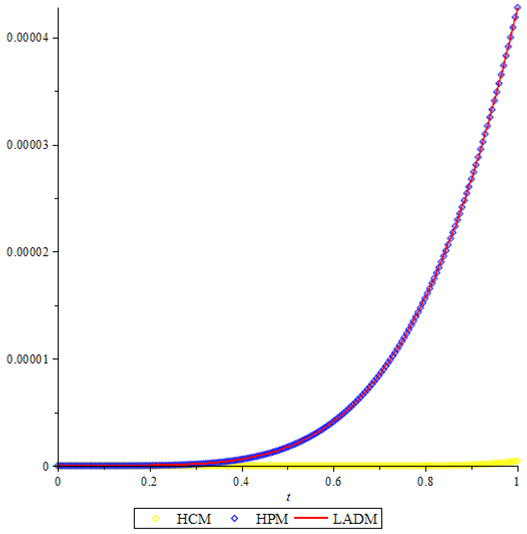
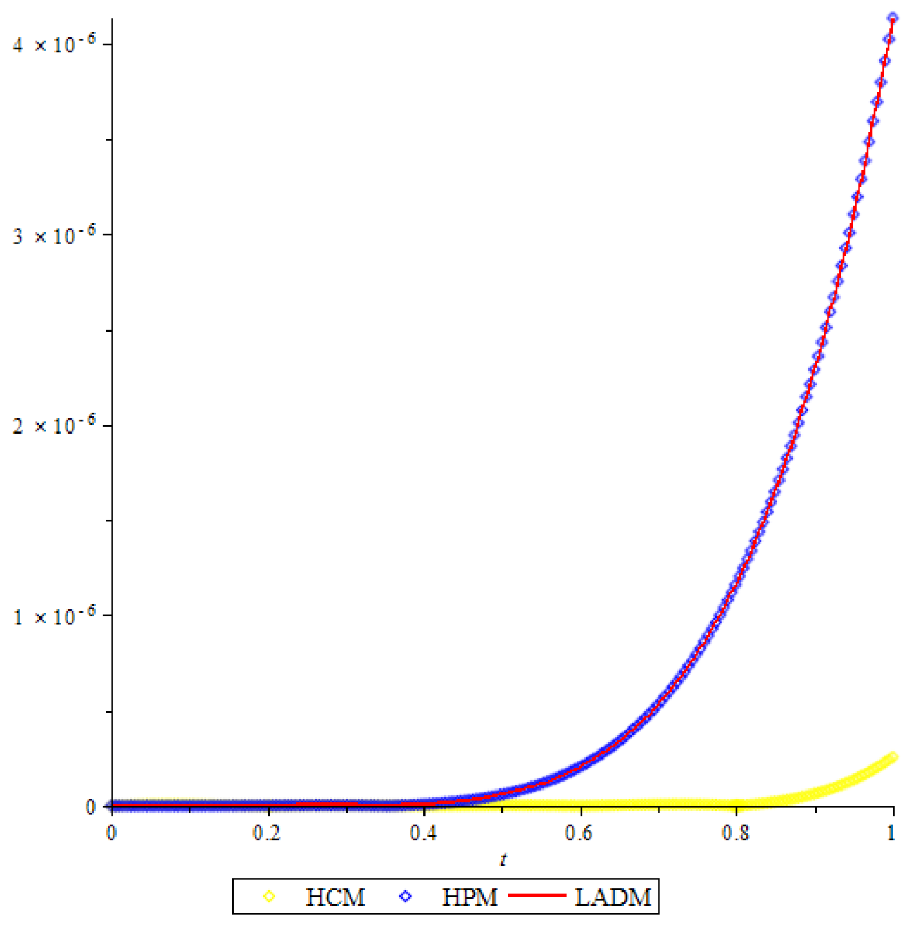
From Figure 1, Figure 2 and Figure 3, it is clear that the results obtained using HCM is very efficient.

5. Conclusions

In this study, the Hermite Collocation Method was applied to obtain the approximate solutions of SIR model. We showed the accuracy and efficiency of the presented method with an example. To show the correctness of the obtained approximate solutions, we put the obtained approximate solutions back into Equation (1) with the aid of Maple software. Thus, it gives extra measure for confidence of the obtained approximate solutions. The obtained approximate results and the error values are compared with the error values and the approximate solutions obtained with homotopy perturbation method (HPM) [10] and Laplace-Adomian decomposition method [12]. These comparisons reveal that our method is more efficient and useful to find approximate solution the SIR model of epidemics. From Table 1, Table 2 and Table 3, it is seen that the numerical solutions of the HPM [10] and the LADM [12] are almost same. Therefore, it is observed that the presented method is an alternative way for the solution of nonlinear ODEs system that have no analytic solution. The greatest advantage of the presented method is that all of above computations can be computed easily in very shorter time by using the computer code written in Maple software.

Author Contributions

All authors contributed equally to the writing of this paper. All authors read and approved the final manuscript.

Funding

This research received no external funding.

Conflicts of Interest

The authors declare no conflict of interest.

References

  1. Hojjati, G.; Ardabili, M.R.; Hosseini, S.M. A-EBDF: An adaptive method for numerical solution of stiff systems of ODEs. Math. Comput. Simul. 2004, 66, 33–41. [Google Scholar] [CrossRef]
  2. Mastorakis, N.E. Numerical solution of non-linear ordinary differential equations via collocation method (finite elements) and genetic algorithms. WSEAS Trans. Inf. Sci. Appl. 2005, 2, 467–473. [Google Scholar]
  3. Shawagfeh, N.; Kaya, D. Comparing numerical methods for the solutions of systems of ordinary differential equations. Appl. Math. Lett. 2004, 17, 323–328. [Google Scholar] [CrossRef]
  4. Yüzbaşı, Ş.; Karaçayır, M. An exponential Galerkin method for solutions of HIV infection model of CD4+ T-cells. Comput. Biol. Chem. 2017, 67, 205–212. [Google Scholar] [CrossRef] [PubMed]
  5. Yüzbaşı, Ş. An exponential collocation method for the solutions of the HIV infection model of CD4+ T cells. Int. J. Biomath. 2016, 9, 885–893. [Google Scholar] [CrossRef]
  6. Al-Omari, A.; Schüttler, H.B.; Arnold, J.; Taha, T. Solving nonlinear systems of first order ordinary differential equations using a Galerkin finite element method. IEEE Access 2013, 1, 408–417. [Google Scholar] [CrossRef]
  7. Arqub, O.A.; El-Ajou, A. Solution of the fractional epidemic model by homotopy analysis method. J. King Saud Univ.-Sci. 2013, 25, 73–81. [Google Scholar] [CrossRef]
  8. Fadi, A.; Adawi, A.; Mustafa, Z. Solutions of the SIR models of epidemics using HAM. Chaos Soliton Fract. 2009, 42, 3047–3052. [Google Scholar]
  9. Biazar, J. Solution of the epidemic model by Adomian decomposition method. Appl. Math. Comput. 2006, 173, 1101–1106. [Google Scholar] [CrossRef]
  10. Rafei, M.; Ganji, D.D.; Daniali, H. Solution of the epidemic model by homotopy perturbation method. Appl. Math. Comput. 2007, 187, 1056–1062. [Google Scholar] [CrossRef]
  11. Ibrahim, S.F.M.; Ismail, S.M. Differential Transformation Approach to a SIR Epidemic Model with Constant Vaccination. J. Am. Sci. 2017, 8, 764–769. [Google Scholar]
  12. Dogan, N.; Akin, Ö. Series solution of epidemic model. TWMS J. Appl. Eng. Math. 2012, 2, 238–244. [Google Scholar]
  13. Harman, D.B.; Johnston, P.R. Applying the stochastic galerkin method to epidemic models with uncertainty in the parameters. Math. Biosci. 2016, 277, 25–37. [Google Scholar] [CrossRef] [PubMed]
  14. Kousar, N.; Mahmood, R.; Ghalib, M.A. Numerical Study of SIR Epidemic Model. Int. J. Sci. Basic Appl. Res. 2012, 25, 354–363. [Google Scholar]
  15. Hussain, R.; Ali, A.; Chaudary, A.; Jarral, F.; Yasmeen, T.; Chaudary, F. Numerical solution for mathematical model of Ebola Virus. Int. J. Adv. Res. 2017, 5, 1532–1538. [Google Scholar] [CrossRef]
  16. Pirim, A.N.; Şahin, N.; Sezer, M. A Hermite collocation method for the approximate solutions of high order linear Fredholm integro-differential equations. Numer. Methods Part. Differ. Equat. 2011, 6, 1707–1721. [Google Scholar]
  17. Pirim, A.N.; Ayaz, F. A New Technique for Solving Fractional Order Systems: Hermite Collocation Method. Springer Phys. Math. Stat. 2016, 7, 2307. [Google Scholar] [CrossRef]
  18. Gülsu, M.; Yalman, H.; Öztürk, Y.; Sezer, M. A New Hermite Collocation Method for Solving Differential Difference Equations. Appl. Appl. Math. 2011, 6, 1856–1869. [Google Scholar]
  19. Pirim, N.A.; Ayaz, F. Hermite collocation method for fractional order differential equations. IJOCTA 2018, 8, 228–236. [Google Scholar]
  20. Ibis, B.; Bayram, M. Numerical solution of the neutral functional-differential equations with proportional delays via collocation method based on Hermite polynomials. Commun. Math. Model. Appl. 2016, 1, 22–30. [Google Scholar]
  21. Gülsu, M.; Sezer, M. On the solution of the Riccati Equation by the Taylor Matrix Method. Appl. Math. Comput. 2006, 176, 414–421. [Google Scholar] [CrossRef]
  22. Erdem, K.; Yalçınbaş, S. Bernoulli Polynomial Approach to HighOrder Linear Differential-Difference Equations. AIP Conf. Proc. 2012, 1479, 360–364. [Google Scholar]
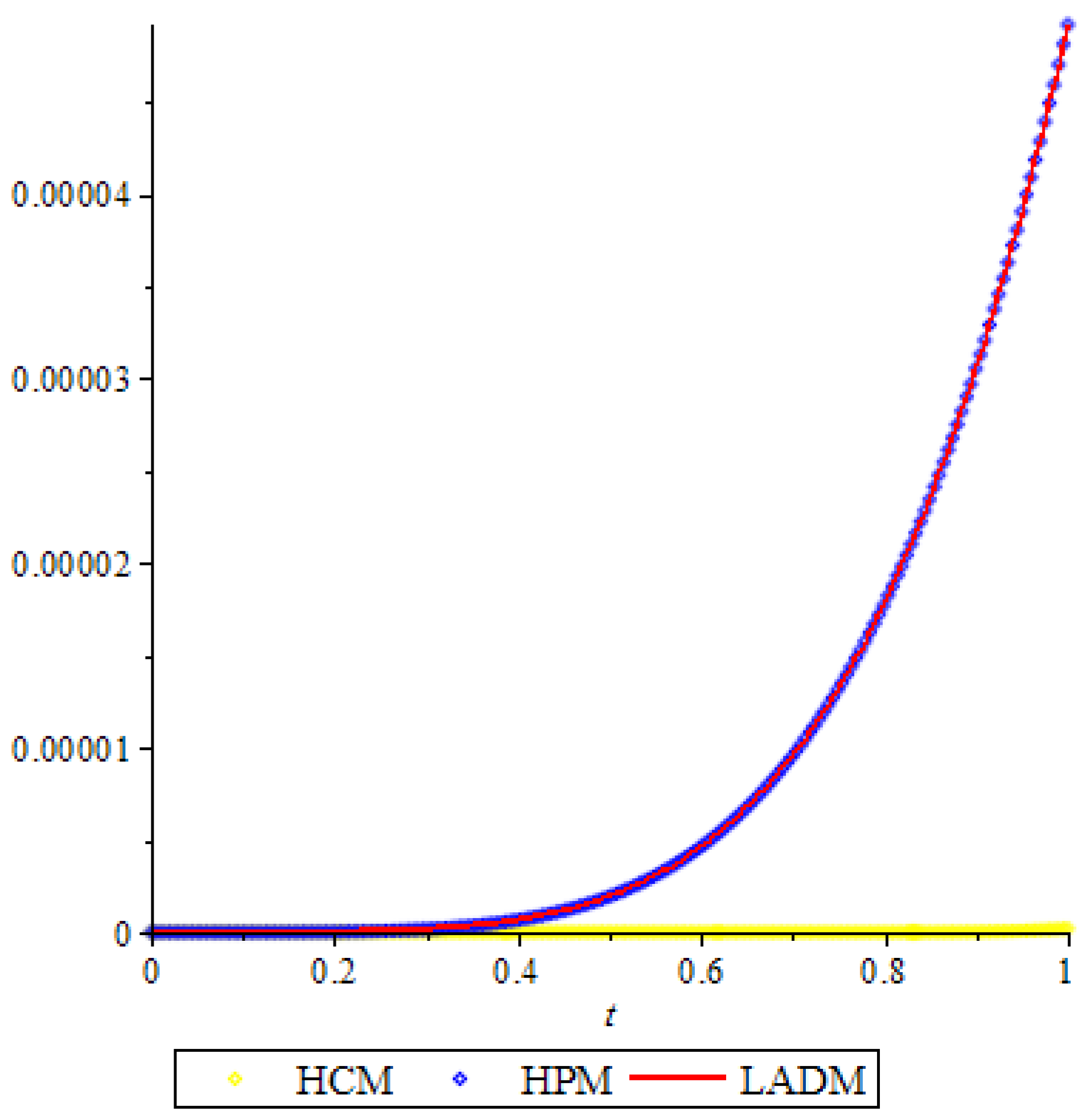
Figure 1. Comparison of the error function E 1 , 5 ( t ) for S(t).
Mathematics 06 00305 g001
Figure 2. Comparison of the error function E 2 , 5 ( t ) for I(t).
Mathematics 06 00305 g002
Figure 3. Comparison of the error function E 3 , 5 ( t ) for R(t).
Mathematics 06 00305 g003
Table 1. The values of S ( t ) , and the residual errors E R S for HPM, HCM and LADM.
t S ( t ) (HPM) ER S (HPM) S ( t ) (HCM for L = 5) ER S (HCM for L = 5) S ( t ) (LADM) ER S (LADM)
0.219.39842557 2.241556564 × 10 8 19.39842556 1.007967528 × 10 9 19.39842557 2.241715696 × 10 8
0.319.09671302 1.639339936 × 10 7 19.09671301 5.224692456 × 10 9 19.09671302 1.639420311 × 10 7
0.418.79461232 6.642448998 × 10 7 18.79461227 1.020070225 × 10 9 18.79461232 6.642702518 × 10 7
0.518.49229607 1.945779417 × 10 6 18.49229590 4.808788220 × 10 9 18.49229607 1.945841205 × 10 6
0.618.18993727 4.638804798 × 10 6 18.18993677 1.036285111 × 10 9 18.18993727 4.638932739 × 10 6
0.717.88770892 9.586736659 × 10 6 17.88770774 2.046575227 × 10 9 17.88770892 9.586973403 × 10 6
0.817.58578366 1.783241468 × 10 5 17.58578115 1.056548098 × 10 9 17.58578366 1.783281825 × 10 5
0.917.28433338 3.058543511 × 10 5 17.28432849 2.255631029 × 10 8 17.28433338 3.058608116 × 10 5
1.016.98352883 4.917070631 × 10 5 16.98352001 1.991812037 × 10 7 16.98352883 4.917169073 × 10 5
Table 2. The values of I ( t ) , and the residual errors E R I for HPM, HCM and LADM.
t I ( t ) (HPM) ER I (HPM) I ( t ) (HCM for L = 5) ER I (HCM for L = 5) I ( t ) (LADM) ER I (LADM)
0.215.54049369 2.037288852 × 10 8 15.54049370 1.007967528 × 10 9 15.54049369 2.037528176 × 10 8
0.315.81085489 1.484224142 × 10 7 15.81085488 5.224692456 × 10 9 15.81085489 1.484345163 × 10 7
0.416.08106363 5.988792320 × 10 7 16.08106367 1.020070225 × 10 9 16.08106363 5.989174454 × 10 7
0.516.35094781 1.746299230 × 10 6 16.35094797 4.808788220 × 10 9 16.35094781 1.746392455 × 10 6
0.616.62033527 4.142434258 × 10 6 16.62033570 1.036285111 × 10 9 16.62033527 4.142627465 × 10 6
0.716.88905418 8.513884329 × 10 6 16.88905522 2.046575227 × 10 9 16.88905418 8.514242143 × 10 6
0.817.15693346 1.574071331 × 10 5 17.15693567 1.056548098 × 10 9 17.15693345 1.574132364 × 10 5
0.917.42380311 2.681612132 × 10 5 17.42380741 2.255631029 × 10 8 17.42380310 2.681709896 × 10 5
1.017.68949465 4.278734031 × 10 5 17.68950236 1.991812037 × 10 7 17.68949464 4.278883073 × 10 5
Table 3. The values of R ( t ) , and the residual errors E R R for HPM, HCM and LADM.
t R ( t ) (HPM) ER R (HPM) R ( t ) (HCM for L = 5) ER R (HCM for L = 5) R ( t ) (LADM) ER R (LADM)
0.210.06108073 1.55732288 × 10 9 10.06108073 1.780152 × 10 12 10.06108073 1.5573248 × 10 9
0.310.09243209 2.71342062 × 10 9 10.09243209 2.99878840 × 10 9 10.09243209 2.7134352 × 10 9
0.410.12432405 7.76566784 × 10 9 10.12432405 3.55561 × 10 12 10.12432405 7.7656064 × 10 9
0.510.15675613 5.88551875 × 10 8 10.15675613 2.9916773 × 10 9 10.15675613 5.88550000 × 10 8
0.610.18972750 2.047705402 × 10 7 10.18972751 5.3304 × 10 12 10.18972750 2.047700736 × 10 7
0.710.22323698 5.326273240 × 10 7 10.22323703 6.997166 × 10 9 10.22323698 5.32626315 × 10 7
0.810.25728304 1.170101371 × 10 6 10.25728317 7.109 × 10 12 10.25728304 1.170099405 × 10 6
0.910.29186379 2.293088789 × 10 6 10.29186411 6.2910522 × 10 8 10.29186379 2.293085246 × 10 6
1.010.32697698 4.133366 × 10 6 10.32697760 4.548599737 × 10 7 10.32697698 4.13336 × 10 6