Tunneling Time in Attosecond Experiments and Time Operator in Quantum Mechanics

Abstract

Attosecond science is of a fundamental interest in physics. The measurement of the tunneling time in attosecond experiments, offers a fruitful opportunity to understand the role of time in quantum mechanics (QM). We discuss in this paper our tunneling time model in relation to two time operator definitions introduced by Bauer and Aharonov–Bohm. We found that both definitions can be generalized to the same type of time operator. Moreover, we found that the introduction of a phenomenological parameter by Bauer to fit the experimental data is unnecessary. The issue is resolved with our tunneling model by considering the correct barrier width, which avoids a misleading interpretation of the experimental data. Our analysis shows that the use of the so-called classical barrier width, to be precise, is incorrect.

1. Introduction

The paper concerns the time operator in relation to the definitions introduced by Bauer [1] and Aharonov–Bohm [2]. Attosecond science (attosecond = 10${}^{-18}$ s) concerns primarily electronic motion and energy transport on atomic scales. In previous work [3,4,5], we presented a tunneling model and a formula to calculate the tunneling time (T-time) by exploiting the time-energy uncertainty relation (TEUR), precisely that time and energy are a (Heisenberg) conjugate pair. Our tunneling time is in a good agreement with the attosecond (angular streaking) experiment for the He atom [3] with the experimental finding of Eckle et al. [6,7,8] and for the hydrogen atom [9] with the experimental finding of Sainadh et al. [10]. Our model presents a real T-time picture or a delay time with respect to the ionization at atomic field strength $F_a$ (see below; compare Figure 1). It is also interesting for the tunneling theory in general, because of its relation to the height of the barrier [3,4].

Indeed, the role of time has been controversial since the appearance of quantum mechanics (QM). The famous example is the Bohr–Einstein weighing photon box Gedanken experiment (BE-photon-box-GE) [11], in which a photon is allowed to escape from a box through a hole, which is closed and opened temporarily by a shutter. The period of time is determined by a clock, which is part of the box system. This means that the time is intrinsic and dynamically connected with the system under consideration. The total mass of the box before and after a photon passes is measured, which leads to uncertainty in the gravitational field, hence an uncertainty in time. Our tunneling time picture [3] shows an intriguing similarity to the BE-photon-box-GE (see for example [12], p. 132), where the former can be seen as a realization of the latter.

Concerning the time operator in QM, recently, Galapon [13,14,15] has shown that there is no a priori reason to exclude the existence of a self-adjoint time operator, canonically conjugate to a semibounded Hamiltonian, contrary to the (famous) claim of Pauli. The result is, as noted earlier by Garrison [16], for a canonically conjugate pair of operators of a Heisenberg type (i.e., uncertainty relation), that Pauli theorem does not apply; unlike a pair of operators that form a Weyl pair (or Weyl system.)

Our simple tunneling model was introduced in [3] (see Figure 1, below). In this model, an electron can be ionized by a laser pulse with an electric field strength (hereafter, field strength) F. Ionization happens directly when the field strength is larger than a threshold called the atomic field strength $F_a=I_p^2/\left(4Z_{eff}\right)$ [17,18], where $I_p$ is the ionization potential of the system (atom or molecule) and $Z_{eff}$ is the effective nuclear charge in the single-active electron approximation. However, for field strengths $F<F_a$, ionization can happen by a tunneling mechanism, through a barrier built by the effective potential due to the Coulomb potential of the nucleus and the electric field of the laser pulse. It can be expressed in a one-dimensional form:

$$V_{eff}\left(x\right)=V\left(x\right)-xF=-\frac{Z_{eff}}{x}-xF;$$

(1)

compare Figure 1. In this model, the tunneling process can be described solely by the ionization potential $I_p$ of the valence (the interacting) electron and the peak field strength F, which leads to the quantity ${\delta }_z=\sqrt{I_p^2-4Z_{eff}F}$, where F stands (throughout this work) for the peak electric field strength at maximum. In Figure 1 (for details, see [3]), the inner (entrance $x_{e,-}$) and outer (exit $x_{e,+}$) point $x_{e,\pm }=(I_p\pm \delta )/\left(2F\right)$, the barrier width $d_W=x_{e,+}-x_{e,-}={\delta }_z/F$ and the barrier height $\left(\mathrm{at} x=x_m\left(F\right)=\sqrt{Z_{eff}/F}\right)$ is $h_B\left(x_m\right)=\mid -I_p-V_{eff}\left(x_m\right)\mid =\mid -I_p+\sqrt{4Z_{eff}F}\mid$. The barrier disappear for ${\delta }_z=0$ ($d_W=0,h_B\left(x_m\right)=0$) at the atomic field strength $F=F_a$, where the direct ionization starts, the barrier-suppression ionization.

In the (low-frequency) attosecond experiment, the laser field is comparable in strength to the electric field of the atom. Usually, intensities of ∼${10}^{14}$ W·cm${}^{-2}$ are used. A key quantity is the Keldysh parameter [19],

$${\gamma }_K=\frac{\sqrt{2I_p}}{F}{\omega }_0={\tau }_K{\omega }_0,$$

(2)

where ${\omega }_0$ is the central circular frequency of the laser pulse and ${\tau }_K$ denotes the Keldysh time. In Equation (2) and hereafter, we adopt the atomic units (au), where the electron’s mass and charge and the Planck constant are set to unity, $\hslash =m=e=1$. In Equation (2), at values ${\gamma }_K>1$, the dominant process is the multiphoton ionization (MPI). On the opposite side, i.e., for ${\gamma }_K<1$, the ionization (or field-ionization) happens by a tunneling process, which occurs for $F<F_a$. This is the famous Keldysh result [19]. In the tunneling process (for $F<F_a$), the electron does not have enough energy to ionize directly. The electron tunnels (tunnel ionizes) through a barrier made by the Coulomb potential and the field of the laser pulse. The electron escapes the barrier at the exit point $x_{e,+}$ to the continuum, as shown in Figure 1 (a sketch for He atom). For our discussion later, we mention that in the experiment of [6], an elliptically-polarized laser pulse was used with ${\omega }_0=0.0619au(\lambda =736$ nm) and with ellipticity $ϵ=0.87$. The electric field strength was varied in the range $F=0.04-0.11$ and for He atom $I_p=0.90357$ au. In the attosecond angular streaking experiment, one uses a close-to-circular polarized laser pulse; the direction of laser field ensures a unique relationship between the time at which the electron exits the tunnel and the direction of its momentum after the laser pulse. The measured momentum vector of the electron hence serves as the hand of a clock (attoclock), which indicates (the streaking angle) the time when the electron appeared from the tunnel in the laser field. It determines the time (streaking angle divided by the laser frequency) the electron has spent in the tunnel in the classically forbidden region inside the potential wall. This difference or delay is referred to as the tunneling delay time. It has to be mentioned that the nonadiabatic effects lead to large measurement error, reflected in large error bars. Compare [6], and see Section 3.3. The impact of deriving pulse parameters (shape, duration, amplitude) can, however, be controlled by choosing optimal pulse parameters, and the readout error can be minimized, as shown in [20,21], which is important due to the relation between tunneling and quantum information processing.

2. The Tunneling Time

The tunneling process in the attosecond experiment can be visualized by a simple picture, as shown in Figure 1. This picture is related to the strong field approximation (SFA) or the Keldysh–Faisal–Reiss approximation [19,22,23]; for introductory reviews, see [24,25,26]. The main idea of the SFA is that the tunneled electron escapes the barrier at the exit point $x_{e,+}$ (see Figure 1), with zero kinetic energy. Precisely, the electron velocity along the (opposite) field direction is zero and negligible in the other directions. One neglects the effect of the atomic potential in the under-the-barrier region (see also [27]. The electron wave function after $x_{e,+}$ (the barrier exit) can be then approximated by a type of plane wave called the Volkov state. The result of SFA is of exponential accuracy (i.e., with an approximate pre-factor). It is, however, important to determine the final electron amplitude of the tunneling or ionization. This simple picture (our tunneling model), which is useful to explain the experiment, is strictly true only in the length gauge (see [28,29,30,31]). In a previous work [3], it was shown that the uncertainty in the energy, which is related to the height of the barrier $h_B\left(x_m\right)$, is quantitatively connected to the atomic potential energy at the exit point, $\Delta E\sim \mid V\left(x_e\right)\mid =\mid -Z_{eff}/x_e\mid$, for arbitrary strengths $F\le F_a$.

By exploiting the TEUR $\Delta E·\Delta T\ge 1/2$, we obtained what we call the symmetrical (or total) T-time: [3]:

$${\tau }_T^{\mathrm{sym}}=\frac{1}{2}\left(\frac{1}{(I_p+{\delta }_z)}+\frac{1}{(I_p-{\delta }_z)}\right)=\frac{I_p}{4Z_{eff}F}$$

(3)

In this relation, ${\delta }_z=\sqrt{I_p^2-4Z_{eff}F}$ for a single active electron model (for the hydrogen atom, $Z_{eff}=1$); for details, see [3,4,9]. The symmetrical T-time or the total time was obtained by a symmetrization procedure (similar to the Aharonov time operator [2,11]; see Section 3.2) from the unsymmetrized (unsymmetrical) T-time relation:

$${\tau }_T^{\mathrm{unsy}}=\frac{1}{(I_p-{\delta }_z)}$$

(4)

Equation (3), besides its mathematical simplicity, aids in the conceptual reasoning [3,4]. The physical reasoning is the following: the barrier itself causes a delaying time ${\tau }_{T,d}$, where:

$${\tau }_{T,d}=\frac{1}{2(I_p-{\delta }_z)},{\tau }_{T,i}=\frac{1}{2(I_p+{\delta }_z)}$$

(5)

${\tau }_{T,d}$ presents the time delay with respect to the ionization at atomic field strength $F_a$, where the barrier is absent (the barrier height, the barrier width $d_W={\delta }_z/F$ and ${\delta }_z$ are zero). It is the time duration for a particle to pass the barrier region (between $x_{e,-},x_{e,+}$) and escape at the exit point $x_{e,+}$ to the continuum [3]. The first term ${\tau }_{T,i}$ in Equation (3) is the time needed to reach the entrance point $x_{e,-}$ from the initial point $x_i$; compare Figure 1. At the limit $F\to F_a({\delta }_z\to 0)$, the total time becomes the ionization time ${\tau }_T^{\mathrm{sym}}=1/I_p$ or ${\tau }_{T,d}={\tau }_{T,i}=1/\left(2I_p\right)$ at the atomic field strength $F_a$. For $F>F_a$, the barrier-suppression ionization sets up [32,33]. At the opposite side, i.e., for $F\to 0$, ${\delta }_z\to I_p$ and ${\tau }_{T,d}\to \infty$, hence nothing happens (undisturbed electron), and the electron remains in its ground state, which shows that our model is consistent. For details, see [3,4,5].

3. Time Operator

In the early days of the QM, a TEUR (analogous to the position-momentum relation) and the existence of the time operator faced the well-known objection of Pauli. According to the Pauli theorem, the introduction of the time operator is basically forbidden, and the time t in QM must necessarily be considered as an ordinary number (‘c’ number). On the other hand, the famous example and its debate is the BE-photon-box-GE. The crucial point is that, to date, no general time operator has been found [34]; thus, a sort of time operator and the uncertainty relation are used dependent on the study cases [35]. There is still a common opinion that time plays a role essentially different from the role of the position in QM (although, this is not in line with special relativity). Hilgevoord concluded in his work [36] that when looking to a time operator, a distinction must be made between universal time coordinate, the t, a c-number like a space coordinate and the dynamical time variable of a physical system situated in space-time; i.e., clocks. The search for a time operator has a long history [37,38,39]. This led Busch [40,41] to classify three types of time in QM: external time (parametric or laboratory time), intrinsic or dynamical time and observable time. In our case study, the time, and hence the tunneling time, is intrinsic or dynamical type [4].

3.1. Bauer’s Time Operator

Bauer [1,42] introduced a dynamical self-adjoint time operator in the framework of Dirac’s relativistic quantum mechanics (DRQM). Bauer’s time operator (BTO) is defined as the following,

$$\widehat{T}=\alpha ·\widehat{\mathit{r}}/c+\beta {\tau }_0$$

(6)

where $\alpha ,\beta$ are the well-known Dirac matrices, c the speed of light and $\mathbf{r}$ the three-dimensional space vector. ${\tau }_0$ represents in principle an internal property of the system, determined to be the de Broglie period $\hslash /\left(m_0{c}^2\right)$ (ℏ is the Planck constant, and $m_0$ is the rest mass of the particle). ${\tau }_0$ is not important for our discussion, since it cancels for time intervals, or time differences.

The operator defined in Equation (6) has been shown to commute with the Dirac free particle Hamiltonian $H_D=c\alpha ·\widehat{p}+\beta m_0{c}^2$. Bauer proved the Heisenberg commutation relation, analyzed the dynamical character of $\widehat{T}$ and found for a free particle:

$$\begin{array}{ccc}\hfill \widehat{T}\left(t\right)& =& {\left(\frac{v_{gp}}{c}\right)}^{2}t+\left(\frac{m_0{c}^2}{H_D}\right){\tau }_0\hfill \end{array}$$

(7)

$$\begin{array}{ccc}\hfill r\left(t\right)& =& v_{gp}t\hfill \end{array}$$

(8)

$$\begin{array}{ccc}\hfill dr\left(t\right)& =& v_{ph}dT\left(t\right)\hfill \end{array}$$

(9)

where $v_{gp}$ is the group and $v_{ph}$ (Equation (9), see Bauer [42]) is the phase velocity of the particle. According to Bauer, $T\left(t\right)$ is the internal time and t the external (laboratory) time, where $T\left(t\right)<t$. In the limit, $m_0=0$, then $v_{gp}=c$ and $T\left(t\right)=t$. The parametric time t, according to Bauer, can be interpreted as the laboratory time, which is the time variable appearing in the time-dependent Schrödinger equation and characterizing the dynamical evolution of microscopical systems

Bauer argued that DRQM allows the introduction of a dynamical time operator that is self-adjoint, unlike the parametric time entering in the Schrödinger equation, while Galapon [13,14,15] showed that in non-relativistic QM (NRQM), there is no reason to exclude the existence of a time operator for a Heisenberg pair, and consequently an observable of time and a dynamical time, as already mentioned.

For a non-relativistic particle, Bauer found [1] a relation between the parametric (external in Bauer’s notation) time intervals and the dynamical (internal in Bauer’s notation) intervals,

$$\begin{array}{ccc}\hfill \Delta T_B& =& <T_B\left(t_2\right)>-<T_B\left(t_1\right)>\hfill \\ \hfill & =& \frac{1}{2}{\left(\frac{v_{gp}}{c}\right)}^2(t_2-t_1)<<(t_2-t_1)=\Delta t_B\hfill \end{array}$$

(10)

The parametric time interval $\Delta t$ is enhanced relative to the internal time interval $\Delta T$, which by the virtue of Equation (6) is related to the time the light takes to travel the same distance. On the other hand, for high (“relativistic”) energies, one obtains:

$$\Delta T_B=<T_B\left(t_2\right)>-<T_B\left(t_1\right)>=(t_2-t_1)=\Delta t$$

In other words, in the relativistic case, internal time intervals coincide with external time intervals, whereas in the non-relativistic case, the latter is enhanced relative to the internal time intervals. At this point, it is important to note that in the presence of a potential dependent only on position, e.g., Coulomb type potentials,

$$[\widehat{T},{\widehat{H}}_D+V\left(\tilde{r}\right)]=[\widehat{T},{\widehat{H}}_D];$$

(11)

hence, the commutation relation of the time operator is reduced to the commutation relation with the relativistic free particle of Dirac operator ${\widehat{H}}_D$, since the latter is a linear function of relativistic momentum $\widehat{p}$. From Equation (6), one finds that Equation (11) is reduced to the position momentum commutation relation $[\widehat{r},\widehat{p}]$.

For the tunneling in the attosecond experiment, Bauer uses the argument of Kullie [3] that the potential energy at the exit point defines the uncertainty in the energy, leads to the time of passage of the barrier or the time needed to cross through the exit point and represents a tunneling internal time of the system ${\tau }_T$. With his view of $\Delta T_B\simeq {\tau }_T$, Bauer obtained a relation for the laboratory time lapse to cross the barrier,

$$\begin{array}{c}\hfill {\mathrm{{\rm Y}}}_T=\frac{1}{4\pi }\xi \frac{1}{\frac{1}{2}{\left(\frac{v_{gp}}{c}\right)}^2}{\tau }_T=\frac{1}{4\pi }2\xi ·\Gamma ·{\tau }_T\end{array}$$

(12)

where $\Gamma ={(v_{gp}/c)}^{-2}$ is called the enhancement factor, $\xi$ is a phenomenological parameter (see below) and ${\tau }_T$ the internal time interval. Compare Equation (10).

Properties of BTO

The BTO is interesting and satisfies the property and the conditions of an ordinary time operator in the relativistic framework of the QM. Despite this, there is an unexpected feature of the relation (12) given by Bauer, as a consequence of the time operator definition in (6). The laboratory time interval $\Delta t$ is connected to the internal time interval $\Delta T\equiv \Delta T_B$ by Equation (12). However, with Equations (6), (8) and (10) and similar to Equation (12):

$$\begin{array}{ccc}\hfill \Delta T_B& =& \Delta \widehat{r}/c=4\pi \Delta \widehat{r}/c=4\pi \Delta r/c\hfill \\ \hfill \Delta t& =& \frac{1}{4\pi }\xi \frac{1}{\frac{1}{2}{\left(\frac{v_{gp}}{c}\right)}^2}\Delta T\hfill \end{array}$$

(13)

Consequently, one finds:

$$\begin{array}{ccc}\hfill \Delta t& =& \frac{1}{4\pi }\frac{c^2}{\frac{1}{2}\left(\frac{\Delta r}{\Delta t}\right)v_{gp}}\left(4\pi \frac{\Delta r}{c}\right)\hfill \end{array}$$

(14)

$$\begin{array}{ccc}\hfill & \hspace{1em}\hspace{1em}\hspace{1em}\hspace{1em}=& \xi \frac{c}{\frac{1}{2}{v}_{gp}}\Delta t\Rightarrow v_{gb}=2\xi c=const\hfill \end{array}$$

(15)

Bauer introduced the phenomenological parameter $\xi <1$ so that ${\mathrm{{\rm Y}}}_T$ in Equation (12) somehow fits the experimental data and the Feynman path integral (FPI) calculation, presented by Landsman [6]; compare Figure 1 of [1] (the same plot is given in Figure 3, Section 3.3). He concluded that $\xi =0.45$ gives the best fit to the experiment. The result of Bauer fits the FPI result of Landsman [6] well; see Figure 1 in [1] (as in Figure 3, Section 3.3). However, there is no theoretical justification for the choice of $\xi$ as a parameter or its value $\xi =0.45$. This is a rather unexpected result, then without the parameter $\xi$ (i.e., $\xi =1$), one obtains $v_{gb}=2c$, which is a consequence of the definition in Equations (6) and (12), where the speed of light is used in the denominator. In other words, the value $\xi =0.5$ gives $v_{gb}=c$, as it should be in accordance with the definition in Equation (6). The idea of Bauer to set a universal internal time Equation (6) is reasonable; however, using it to measure external time intervals, i.e., the relation between internal time intervals and external time intervals Equation (12), leads to unexpected implications. We will see that our tunneling model and our definition, or the generalization of time operators of Bauer and Aharonov (see below), clarifies this implication and that there is no need to introduce a phenomenological parameter.

3.2. Time Operator of the Type Aharonov–Bauer

The recent interesting work of Bauer and the introduction of a time operator in the frame work of the DRQM, together with the well-known Aharonov time operator (Equation (19) below), have stimulated us to define a generalized form of the time operator(s) of the same types. We suggest that the time operator definition of Aharonov and Bauer can be extended and combined as the following. For one particle (in atomic units):

$${\widehat{t}}_{gp}=\mathbf{\alpha }\frac{\widehat{\mathbf{r}}}{v_{gp}},{\widehat{t}}_{ph}=\mathbf{\alpha }\frac{\widehat{\mathbf{r}}}{v_{ph}}$$

(16)

where $v_{ph}$, $v_{gp}$ are the phase and the group velocity, respectively. In the following, we look to a one-dimensional case with the radial coordinate r, i.e., we neglect the factor $1/\left(4\pi \right)$ used by Bauer of the three-dimensional case, where $\mathbf{r}=4\pi r$. The Dirac matrices $\alpha$ will be set to unity $\alpha =1$. Under the definition in Equation (16), the notation internal, external time operator is misleading. We denote ${\widehat{t}}_{gp}$ the dynamical time operator (dynamical TO) and ${\widehat{t}}_{ph}$ the phase (or phase-velocity) time operator (phase TO), without any connection to the notation external, internal time classification of Busch [35]. The relation between the dynamical and phase times follows immediately from Equation (16), using an interval $\Delta r=\Delta t_{ph}·v_{ph}=\Delta t_{gp}·v_{gp}$.

$$\Delta t_{gp}·v_{gp}=\Delta t_{ph}·v_{ph}\Rightarrow \Delta t_{gp}=\frac{v_{ph}}{v_{gp}}\Delta t_{ph}\ge \Delta t_{ph}$$

(17)

Because of the relativistic relation $v_{ph}{v}_{gp}=c^2$ for a matter particle with a mass m, $E=m{c}^2$, $v_{ph}=E/p$, one obtains ${\widehat{t}}_{gp}\ge {\widehat{t}}_{ph}$, where p is the momentum of the particle. For this reason, it is better to adopt the notations: ${\widehat{t}}_{ph}$ the phase and ${\widehat{t}}_{gp}$ the dynamical time operator. For the light (photon) particle $v_{gp}=v_{ph}=c$, one obtains the BTO:

$${\widehat{t}}_{gp}={\widehat{t}}_{ph}=\alpha \frac{\widehat{r}}{c}$$

(18)

For the non-relativistic one-dimensional case ($\alpha =1$), it is straightforward to obtain the well-known Aharonov–Bohm [2] time operator (ABTO) (${\widehat{t}}_{gp}=\widehat{r}/v_{gp}$) or the quantum mechanical symmetric operator:

$${\widehat{t}}_{gp}=\frac{1}{2}\left(\widehat{r}{v}_{gp}^{-1}+v_{gp}^{-1}\widehat{r}\right)$$

(19)

For ${\widehat{t}}_{ph}$, the symmetrization has no meaning, because $v_{ph}$ is not an observable, unlike $v_{gp}$. The commutation relations were verified in both cases, the non-relativistic Bohm–Aharonov operator [2,43] and the relativistic Bauer operator [1,42]. For ${\widehat{t}}_{ph}$, because $v_{ph}$ is not an observable, the commutation relation is reduced to the known commutation relation $[\widehat{r},\widehat{p}]$.

The first consequence of our definition is the equivalence to the BTO, as given in Equation (18), and to the ABTO Equation (19). There is also an equivalence between BTO and ABTO; then, from Equation (19), for a light particle with $v_{ph}=v_{gp}=c$:

$$\begin{array}{c}\hfill {\widehat{t}}_{gp}=\frac{1}{2}\left(\frac{\widehat{r}}{c}+\frac{\widehat{r}}{c}\right)=\frac{\widehat{r}}{c}\end{array}$$

(20)

and for a matter particle $v_{ph}·v_{gp}=c^2$:

$$\begin{array}{ccc}\hfill \Delta t_{gp}& =& \frac{\Delta r}{v_{gp}}=\frac{v_{ph}·\Delta t_{ph}}{v_{gp}}=\frac{c^2/v_{gp}}{v_{gp}}\Delta t_{ph}\hfill \\ \hfill & =& \frac{1}{{(v_{gp}/c)}^2}\Delta t_{ph}\hfill \end{array}$$

(21)

as already found by Bauer. Compare Equations (7), (12) and (13). No approximation is used, but with $\Delta t_{gp}$ instead of the parametric time $\Delta t$ and $\Delta t_{ph}$ instead the internal time $\Delta T$ of Bauer’s notations.

Bauer obtained the factor $\xi {(1/2)}^{-1}=2\xi$ in Equation (12) by going from relativistic to non-relativistic approximation (the factor ${(1/2)}^{-1}$) and using a phenomenological parameter $\xi$ to fit the experimental data. ${\widehat{t}}_{ph}$ is the phase time, whereas Bauer refers to it as internal time $T_B$ (using $v_{ph}=c$). In the Bauer case (notation), one has $\Delta T_B\le \Delta t_B$; see Equations (10) and (12). Likewise, we have a relation between the dynamical and phase times, $\Delta t_{ph}\le \Delta t_{gp}$, Equation (21). However, one has $T_B=\widehat{r}/c\ge t_{ph}=\widehat{r}/v_{ph}$ because $v_{ph}\ge c$. Further, we get the Bauer procedure for the three-dimensional case by the replacing $\Delta r/c$ with $\Delta r/v_{ph}$, which with $\Delta \mathbf{r}=4\pi \Delta r$, gives Equation (13):

$$\begin{array}{c}\hfill \Delta t_{gp}=(\frac{1}{4\pi })\frac{1}{{(\frac{v_{gp}}{c})}^2}\Delta t_{ph}\end{array}$$

(22)

The only difference between (13) and (22) is that Bauer used $2\xi =2\times 0.45=0.9$ (compare Equations (12) and (13)), whereas it is equal $2\times 0.5$, or exactly $\xi =1/2$ in our case without any approximation. The difference is very small, and $\xi =0.45$ does not fit perfectly to the experimental data of [6]; see below. Thus, referring to $\Delta T=\Delta r/c$ as an internal time and introducing a phenomenological parameter $\xi$ have no justification, unless one relates every time interval to its counterpart of a unique time interval of the light propagation, which is $\Delta r/c$ by replacing the phase time of a matter particle by $v_{ph}=c$; that is straightforward, and a parameter $\xi$ is redundant.

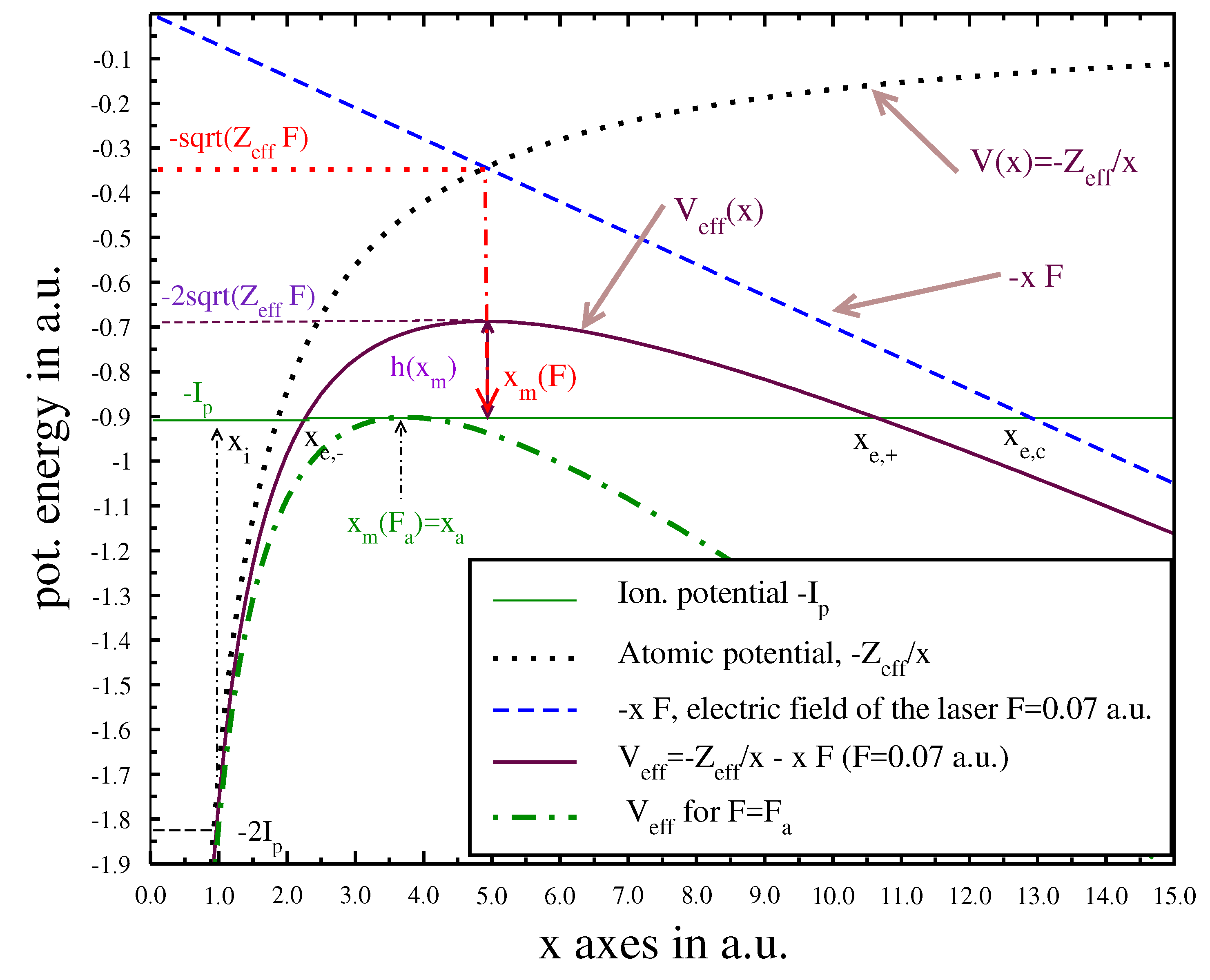
With his approximation, Bauer obtained Equation (12) or (13), whereas on the basis of our tunneling model, Equation (5) can be written, after a small manipulation, in the form (F is the field strength):

$$t_{gp}\left(F\right)\equiv {\mathrm{{\rm Y}}}_K\left(d_W\right)={\tau }_d=\frac{1}{4Z_{eff}}\left(d_W+x_{e,-}\right),$$

(23)

where $d_W={\delta }_z/F$ is the barrier width and $x_{e,-}=(I_p-{\delta }_z)/\left(2F\right)$ [3]; compare Figure 1. In the following, to avoid a confusion, we refer in the general case to a barrier width as $D_{BW}$; Whereas in our model, we set $D_{BW}=d_W$, and for the classical barrier width we set $D_{BW}=d_C$. On the basis of numerical values from the experimental data in [6], with approximate barrier width $d_C$ (compare [6] with [1]) and with the values $d_C=13au$ (in atomic units), $\tau =40as$ (in attosecond), $F\approx 0.069au$, $v_{gb}=13/40(au/as)=6.88/40(\mathrm{\AA }/as)$, Bauer obtained [1],

$$\begin{array}{ccc}\hfill {\mathrm{{\rm Y}}}_B\left(D_{BW}\right)& =& \frac{1}{4\pi }608.44(\mathrm{\AA }/as)\left(\xi \frac{D_{BW}}{c}\right)\hfill \\ \hfill & =& 16.14\times \xi \times D_{BW}as\left(D_{BW}\mathrm{in}\mathrm{\AA }\right)\hfill \\ \hfill & =& 4.52\times \xi \times D_{BW}as\left(D_{BW}\mathrm{in}au\right)\hfill \end{array}$$

(24)

where $D_{BW}$ is a barrier width, Å is Angström length unity and au atomic units. The factor $(2/[{(v_{gb}/c]}^2)=2/{[(6.88/40)/c]}^2=608.44$ is calculated by using the numerical data above, and the best fit to the experimental data according to Bauer is $\xi =0.45$. One notes that Landsman [6] assumed a classical barrier width, i.e., $D_{BW}=d_C=I_p/F$ which is larger than $d_W$ (compare Figure 1). It is usually taken to be approximately valid and is adopted by Bauer. However, as we will see below, this leads to a confusion in the evaluation of the tunneling time against the barrier width; whereas from our model Equations (5) and (23), it follows that ${\tau }_d=3.6(d_W+x_{e,-})as$, using $Z_{eff}=1.6875$ of Clementi [44] (for small barrier width), or ${\tau }_d=4.4(d_W+x_{e,-})as$, using $Z_{eff}=1.375$ of Kullie (for large barrier width) (see [3]); however, no fitting procedure is used, and our ${\tau }_d$ is in good agreement with the experimental data. One can imagine that BTO, Equation (6), presents a universal time scale or internal clock of a light particle, a photon, but its relation to the external time or clocks is then not presented by Equations (12) and (13); see below. We think that our definition is a generalized form, Equation (16), with a straightforward transition to both the BTO and the non-relativistic ABTO.

3.3. Experimental Affirmation

It is worthwhile to mention that the velocity with which the electron passes through the tunnel varies slowly with the barrier width. In our model and with some manipulation, one obtains the mean velocity as a function of $d_W$:

$$\begin{array}{ccc}\hfill \overline{v_{gb}\left(d_W\right)}& =& d_W/{\tau }_d=\frac{d_W}{\frac{1}{2(I_p-{\delta }_z)}}=\frac{d_W}{(d_W+x_{e,-})/4Z_{eff}}\hfill \\ & =& 4Z_{eff}\frac{d_W}{(d_W+x_{e,-})}<4Z_{eff}\hfill \end{array}$$

(25)

For $Z_{eff}=1.6875$, respectively $1.375$, we obtain the values $\overline{v_{gp}\left(d_W\right)}<4Z{e}_{eff}=6.75$, respectively $5.5$. Using the experimental data at one point (see Equation (24)), Bauer extracted a value $(2\times \xi /{(v_{gb}/c)}^2)=\xi \times 608.44$ (compare Equation (22) or $\overline{v_{gp}^C}=(d_C/\tau ){\mid }_{F=0.069}=\left(13au\right)/\left(40as\right)=(13/1.66)au=7.86$ au, which was used as a fixed (independent of F) mean value in Equation (24) independent of the barrier width. It is sightly larger than our values $6.75\left(5.5\right)$, which is caused by the use of the classical barrier width $d_C=I_p/F=d_W+2x_{e,-}$ (compare Equations (12) and (24)), and we think it is one of the reasons why Bauer needed to introduce a phenomenological parameter.

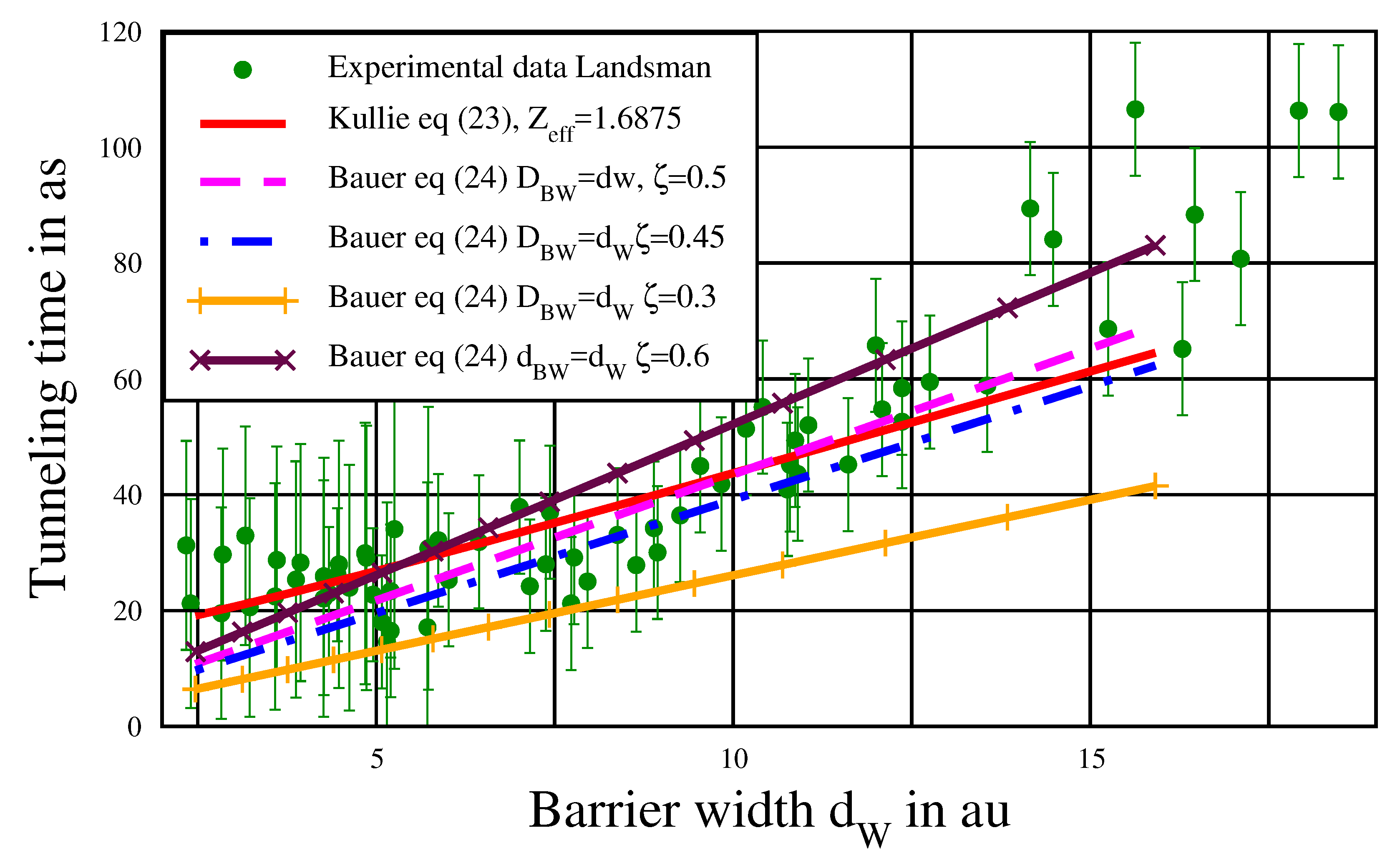
In Figure 2, we plot our result of tunneling time ${\mathrm{{\rm Y}}}_K\left(d_W\right)$, Equation (23), against the barrier width $d_W\left(F\right)={\delta }_z/F$, where $Z_{eff}=1.6875$ is used, together with Bauer’s tunneling time formula ${\mathrm{{\rm Y}}}_B(D_{BW}=d_W)$, Equation (24), with $\xi =0.45$ used by Bauer, with our value $\xi =0.5$ and the values $\xi =0.3,0.6$ used by Bauer. In addition, the experimental tunneling time data (plotted against $D_{BW}=d_W$) together with the error bars are shown. The elementary data or the experimental values of time of [6] (at the corresponding F values) were sent by Landsman, where $d_W$ was easily calculated from $d_W={\delta }_z/F$. As seen in Figure 2, Equation (23) (solid red line) shows the best fit with the experimental data. The dashed (pink) line of Equation (24) with $D_{BW}=d_W$ and $\xi =0.5$ is slightly below the red solid line (for small $d_W$), and the dashed dotted (blue) one of Equation (23) with $D_{BW}=d_W$ and $\xi =0.45$ is slightly below both.

One notices that we used $Z_{eff}=1.6875$, which is suitable for small barrier widths, whereas $Z_{eff}=1.375$ is better for large barrier widths, with which the lines will slightly shift towards higher values. The red line is then closer to the experimental values for large barrier width (compare Figure 5 in [3]), and the pink and blue lines stay below the red line in this region.

Figure 2 has a small difference from the figure shown in [6] (Figure 3d, FPI) and to Figure 1 from [1] (same as Equation (24), with $\xi =0.3,0.45,0.6$). Because in both works, $D_{BW}=d_C=I_p/F=d_W+2x_{e,-}$ was used, where the plotted lines are slightly above the experimental data, i.e., the lines showed less agreement than in our evaluation plotted in Figure 2. In other words, a parameter $\xi$ is not needed, when one uses the correct barrier width $d_W=\delta /F$ (compare Figure 1), and a better agreement with the experimental data is obtained.

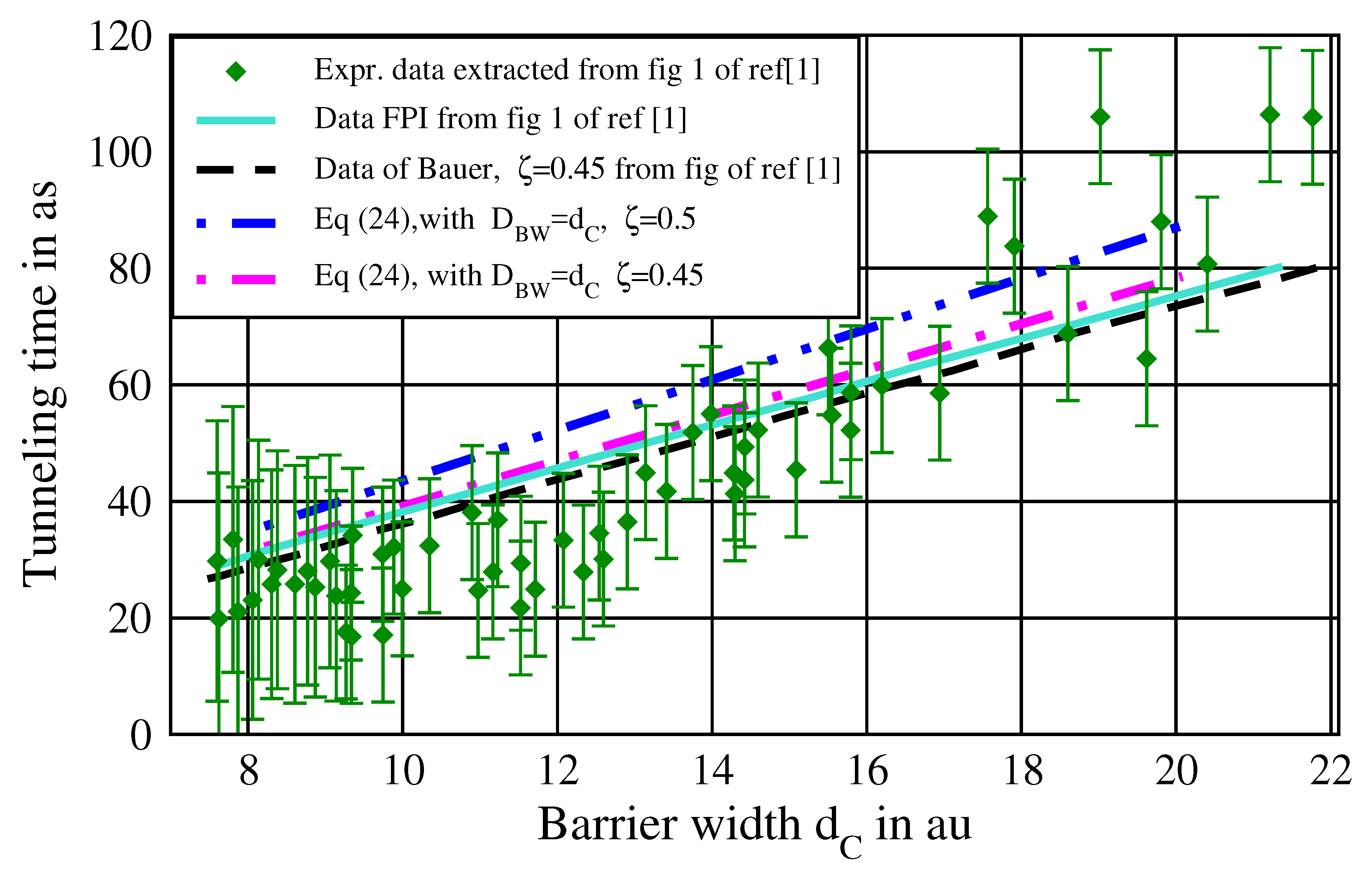
For clarity, we plot in Figure 3 a copy of Figure 1 of [1] (extracted data by using a web digitizer), i.e., the data of Bauer ${\mathrm{{\rm Y}}}_B(D_{BW}=d_C)$ for $\xi =0.45$ (dashed, black) and also the FPI (solid, light blue), which was used by Bauer after it was extracted from Figure 3d of [6]. Additionally, we plot ${\mathrm{{\rm Y}}}_B(D_{BW}=d_C)$ with $\xi =0.45$ (dashed doted, magenta), which as expected, reproduce the line of Bauer (dashed, black); the tiny difference is only because we extracted the data of Figure 1 of Bauer [1] by a web digitizer. Furthermore ${\mathrm{{\rm Y}}}_B(D_{BW}=d_C)$ with $\xi =0.5$ is plotted (dashed dotted dotted, blue), which lies slightly higher. We can reproduce the data of Bauer, which makes our conclusion reliable. Thus, we can see why Bauer found that $\xi =0.45$ fits better to FPI; this is because the use of the approximate barrier width $D_{BW}=d_C$; precisely speaking, the use of $D_{BW}=d_C$ is incorrect. The small difference was not crucial for Landsman in the work [6] (Figure 3d), but Landsman noted that it is an approximate barrier width, unlike our model [3] (published later), where a correct barrier width $D_{BW}=d_W=x_{e,+}-x_{e,-}={\delta }_z/F$ was obtained; compare Figure 1. Our conclusion is that, although the difference between $d_W$ and $d_C$ seems to be not crucial as thought by Landsman [6] (and many other authors, for example [10,45]; see also [9]), the use of a barrier width $D_{BW}=d_C$ instead of $d_W$ leads to confusion and is misleading; especially when plotting the tunneling time data against the barrier. This led Bauer to introduce a parameter with the value $\xi =0.45$, which in our view is unnecessary, regardless of how one understands Bauer’s definition of “internal” time operator in Equation (6). Thus, our definition of a time operator Equation (16) is reasonable; it is a general form with a straightforward transitions to BTO Equation (6) [1,42] and ABTO [2].

As a final note, we demonstrate the importance of our model to the tunneling theory in general, because it relates the tunneling time to the barrier height. The T-time found in Equation (3) can be also derived in a simple way, when we assume that the barrier height corresponds to a maximally-symmetric operator as the following. The barrier height $h_B\left(x_m\right)\equiv h_M$ can be related to an (real) operator ${\widehat{h}}_B\left(x_m\right)$

$${\widehat{h}}_M^{\pm }=-I_p\pm \sqrt{4Z_{eff}F}=-I_p\pm \Delta$$

(26)

and the uncertainty in the energy caused by the barrier:

$${\left({\widehat{h}}_M^{-}{\widehat{h}}_M^{+}\right)}^{1/2}={\left[(-I_p-\Delta )(-I_p+\Delta )\right]}^{1/2}={\delta }_z$$

(27)

From this, we get $\Delta E^{\pm }=abs(-I_p\pm {\delta }_z)$, i.e., we have to add (subtract) the internal energy of the system (the ionization potential). Hence, we get ${\tau }_{T,d}$, ${\tau }_{T,i}$ and ${\tau }_T^{\mathrm{sym}}$ by the virtue of the time-energy uncertainty relation, where we assumed that the time is intrinsic and has to be considered (a delay time) with respect to the ionization (time) at atomic field strength, i.e., with respect to the internal energy or the ionization potential $I_p$. This suggests to consider $h_M$ as a perturbation (energy) operator, where the full operator of the system can be taken as $H_0+h_M^{\pm }$. In fact, one can argue that $-I_p$ must be taken to avoid the divergence of the time to infinity for $F=F_a$, because it is physically incorrect, as ${\delta }_z\left(F_a\right)=0\Rightarrow \tau =1/\left(2{\delta }_z\right)\to \infty$, which in turn, can be seen as an initialization of the internal clock, i.e., the T-time is counted as a delay with respect to the ionization at $F_a$ (the limit of the subatomic field strength), after which no tunneling occurs, and the ionization is classically an allowed process, the barrier-suppression ionization.

Actually, we see immediately from Figure 1 that the maximum of the effective potential curve is equal to $-2\sqrt{Z_{eff}F}$ [3]; it goes lower with increasing field strength, where at $F=F_a$, it becomes $-2\sqrt{Z_{eff}F}=-I_p$ or $I_p^2-4Z_{eff}F=0$. Hence, for $F\le F_a$, one gets $I_p^2-4Z_{eff}F={\delta }_z^2\ge 0$. Now, the distance (or the height) to the $-I_p$ (horizontal line) level (at maximum) is then $\left|h\right|=\sqrt{{\delta }_z^2}$. ${\delta }_z$ presents the change of the potential energy in the barrier region (as it should be) ${\Delta V\left(x\right)|}_{x_{e,-}}^{x_{e,+}}=-Z_{eff}/x_{e,+}-(-Z_{eff}/x_{e,-})={\delta }_z$. Hence, the energy gap $\Delta E^{\pm }=abs(-I_p\pm \left|h\right|)$; from which we get the tunneling time ${\tau }_{T,d}$ and ${\tau }_{T,i}$ by virtue of the TEUR.

4. Conclusions

In this work, we showed that our tunneling time model for the tunneling in the attosecond angular streaking experiment enables us to discuss and understand the time and time operator in quantum mechanics. We found a generalized form of a time operator with straightforward transitions to the Bauer time operator, which was introduced in the framework of relativistic Dirac theory, and to the Aharonov–Bohm time operator, which was introduced in the non-relativistic quantum mechanics. Moreover, we found that the introduction of a phenomenological parameter as done by Bauer is unnecessary. The issue is resolved, where the confusion was caused by the use of the classical barrier width. It is clarified by using the correct barrier width, as found by our tunneling model.

References

1. Bauer, M. Tunneling in attosecond optical ionization and a dynamical time operator. Phys. Rev. A 2017, 96, 022139. [Google Scholar] [CrossRef]
2. Aharonov, Y.; Bohm, D. Time in the Quantum Theory and the Uncertainty Relation for Time and Energy. Phys. Rev. 1961, 122, 1649. [Google Scholar] [CrossRef]
3. Kullie, O. Tunneling time in attosecond experiments and the time-energy uncertainty relation. Phys. Rev. A 2015, 92, 052118. [Google Scholar] [CrossRef]
4. Kullie, O. Tunneling time in attosecond experiments, intrinsic-type of time. Keldysh, and Mandelstam—Tamm time. J. Phys. B Atom. Mol. Opt. Phys. 2016, 49, 095601. [Google Scholar] [CrossRef]
5. Kullie, O. How to understand the tunneling in attosecond experiment?: Bohr–Einstein photon box Gedanken experiment, tunneling time and the wave particle duality. Ann. Phys. 2018, 389, 333–351. [Google Scholar] [CrossRef]
6. Landsman, A.S.; Weger, M.; Maurer, J.; Boge, R.; Ludwig, A.; Heuser, S.; Cirelli, C.; Gallmann, L.; Keller, U. Ultrafast resolution of tunneling delay time. Optica 2014, 1, 343–349. [Google Scholar] [CrossRef]
7. Eckle, P.; Pfeiffer, A.N.; Cirelli, C.; Staudte, A.; Dörner, R.; Muller, H.G.; Büttiker, M.; Keller, U. Attosecond Ionization and Tunneling Delay Time Measurements in Helium. Sience 2008, 322, 1525–1529. [Google Scholar] [CrossRef] [PubMed]
8. Eckle, P.; Smolarski, M.; Schlup, F.; Biegert, J.; Staudte, A.; Schöffler, M.; Muller, H.G.; Dörner, R.; Keller, U. Attosecond angular streaking. Nat. Phys. 2008, 4, 565–570. [Google Scholar] [CrossRef] [Green Version]
9. Kullie, O. Tunneling time in attosecond experiment for hydrogen atom. J. Phys. Commun. 2018, 2, 065001. [Google Scholar] [CrossRef] [Green Version]
10. Sainadh, U.S.; Xu, H.; Wang, X.; Atia-Tul-Noor; Wallace, W.C.; Douguet, N.; Bray, A.W.; Ivanov, I.; Bartschat, K.; Kheifets, A.; et al. Attosecond angular streaking and tunnelling time in atomic hydrogen. arXiv, 2017; arXiv:1707.05445. [Google Scholar]
11. Aharonov, Y.; Reznik, B. “Weighing” a Closed System and the Time-Energy Uncertainty Principle. Phys. Rev. Lett. 2000, 84, 1368. [Google Scholar] [CrossRef] [PubMed]
12. Auletta, G.; Fortunato, M.; Parisi, G. Quantum Mechanics; Cambridge University Press: Cambridge, UK, 2009. [Google Scholar]
13. Galapon, E.A. Pauli’s theorem and quantum canonical pairs: The consistency of a bounded, self-adjoint time operator canonically conjugate to a Hamiltonian with non—Empty point spectrum. Proc. R. Soc. Lond. A 2002, 458, 451. [Google Scholar] [CrossRef]
14. Galapon, E.A. Self-adjoint time operator is the rule for discrete semi-bounded Hamiltonians. Proc. R. Soc. Lond. A 2002, 458, 2671. [Google Scholar] [CrossRef]
15. Galapon, E.A. What could have we been missing while pauli’s theorem was in force? arXiv, 2003; arXiv:quant-ph/0303106. [Google Scholar]
16. Garrison, J.; Wong, J. Canonically Conjugate Pairs, Uncertainty Relations, and Phase Operators. J. Math. Phys. 1970, 11, 2242. [Google Scholar] [CrossRef]
17. Augst, S.; Strickland, D.; Meyerhofer, D.D.; Chin, S.L.; Eberly, J.H. Tunneling ionization of noble gases in a high-intensity laser field. Phys. Rev. Lett. 1989, 63, 2212. [Google Scholar] [CrossRef] [PubMed]
18. Augst, S.; Meyerhofer, D.D.; Strickland, D.; Chin, S.L. Laser ionization of noble gases by Coulomb-barrier suppression. J. Opt. Soc. Am. B 1991, 8, 858–867. [Google Scholar] [CrossRef]
19. Keldysh, L.V. Ionization in the Field of a Strong Electromagnetic Wave. J. Exp. Theor. Phys. 1964, 47, 1945–1957. [Google Scholar]
20. Pankratov, A.L.; Gavrilov, A.S. Optimal fast single-pulse readout of qubits. Phys. Rev. B 2010, 81, 052501. [Google Scholar] [CrossRef]
21. Zhang, Q.; Kofman, A.G.; Martinis, J.M.; Korotkov, A.N. Analysis of measurement errors for a superconducting phase qubit. Phys. Rev. B 2006, 74, 214518. [Google Scholar] [CrossRef] [Green Version]
22. Faisal, F.H.M. Multiple absorption of laser photons by atoms. J. Phys. B 1973, 6, L89. [Google Scholar] [CrossRef]
23. Reiss, H.R. Effect of an intense electromagnetic field on a weakly bound system. Phys. Rev. A 1980, 22, 1786. [Google Scholar] [CrossRef]
24. Zheltikov, A.M. Keldysh photoionization theory: Through the barriers. Physics (Uspekhi) 2017, 60, 1087. [Google Scholar] [CrossRef]
25. Popruzhenko, S.V. Keldysh theory of strong field ionization: History, applications, difficulties and perspectives. J. Phys. B 2014, 47, 204001. [Google Scholar] [CrossRef]
26. Ivanov, M.Y.; Spanner, M.; Smirnova, O. Anatomy of strong field ionization. J. Mod. Opt. 2005, 52, 165. [Google Scholar] [CrossRef]
27. Perelomov, A.M.; Popov, V.S.; Terentév, M.V. Ionization of atoms in a variable electric field. Zh. Eksp. Teor. Fiz. 1966, 50, 1393, [Sov. Phys. JETP 1966, 23, 924]. [Google Scholar]
28. Bauer, D.; Milos̆evíc, D.B.; Becker, W. Strong-field approximation for intense-laser-atom processes: The choice of gauge. Phys. Rev. A 2005, 72, 023415. [Google Scholar] [CrossRef]
29. Faisal, F.H.M. Gauge-invariant intense-field approximations to all orders. J. Phys. B 2007, 40, F145. [Google Scholar] [CrossRef]
30. Faisal, F.H.M. Gauge-equivalent intense-field approximations in velocity and length gauges to all orders. Phys. Rev. A 2007, 75, 063412. [Google Scholar] [CrossRef]
31. Reiss, H. R. The tunnelling model of laser-induced ionization and its failure at low frequencies. J. Phys. B 2014, 47, 204006. [Google Scholar] [CrossRef] [Green Version]
32. Delone, N.B.; Kraǐnov, V.P. Tunneling and barrier-suppression ionization of atoms and ions in a laser radiation field. Physics (Uspekhi) 1998, 41, 469–485. [Google Scholar] [CrossRef]
33. Kiyan, I.Y.; Kraǐnov, V.P. Above-barrier ionization of the hydrogen atom in a superstrong optical field. Sov. Phys. JETP 1991, 73, 429–430. [Google Scholar]
34. Dodonov, V.V.; Dodonov, A.V. Energy-time and frequency-time uncertainty relations: Exact inequalities. Phys. Scr. 2015, 90, 074049. [Google Scholar] [CrossRef]
35. Busch, P. Time in Quantum Mechanics—Vol. 1. In Lecture Notes in Physics; Muga, J.G., Mayato, R.S., Egusquiza, I.L., Eds.; Springer: Berlin, Germany, 2008; Volume 734, pp. 73–105. [Google Scholar]
36. Hilgevoord, J. Time in quantum mechanics. Am. J. Phys. 2002, 70, 301. [Google Scholar] [CrossRef]
37. Razavy, M. Quantum-Mechanical Time Operator. Am. J. Phys. 1967, 35, 955. [Google Scholar] [CrossRef]
38. Goto, T.; Naka, S.; Yamaguchi, K. On the Time Operator in Quantum Mechanics. II: General Prescription in One Dimensional Case. Prog. Theor. Phys. 1981, 66, 1915–1925. [Google Scholar] [CrossRef]
39. Wang, Z.-Y.; Xiong, C.-D. How to introduce time operator. Ann. Phys. 2007, 322, 2304–2314. [Google Scholar] [CrossRef] [Green Version]
40. Busch, P. On the energy-time uncertainty relation. Part I: Dynamical time and time indeterminacy. Found. Phys. 1990, 20, 1–32. [Google Scholar] [CrossRef]
41. Busch, P. On the energy-time uncertainty relation. Part II: Pragmatic time versus energy indeterminacy. Found. Phys. 1990, 20, 33–43. [Google Scholar] [CrossRef]
42. Bauer, M. A dynamical time operator in Dirac’s relativistic quantum mechanics. Int. J. Mod. Phys. A 2014, 29, 1450036. [Google Scholar] [CrossRef]
43. Paul, H. Über quantenmechanische Zeitoperatoren. Ann. Phys. 1962, 464, 252. [Google Scholar] [CrossRef]
44. Clementi, E.; Raimondi, D.L.J. Atomic Screening Constants from SCF Functions. Chem. Phys. 1963, 38, 2686. [Google Scholar] [CrossRef]
45. Torlina, L.; Morales, F.; Kaushal, J.; Ivanov, I.; Kheifets, A.; Zielinski, A.; Scrinzi, A.; Muller, H. G.; Sukiasyan, S.; et al. Interpreting attoclock measurements of tunnelling times. Nat. Phys. 2015, 11, 503–508. [Google Scholar] [CrossRef] [Green Version]
Figure 1. (Color online) Graphic display of the potential and the effective potential curves, the two inner and outer points x e , ± = ( I p ± δ z ) / 2 F and the barrier width d W = x e , + x e , = δ z / F . δ z = I p 2 4 Z e f f F , and I p is the ionization potential, Z e f f the effective nuclear charge and F the electric field strength of the laser pulse at maximum. x e , c = I p / F d C is the “classical exit” point, x m ( F ) = Z e f f / F is the position at the maximum of the barrier height h ( x m ) , x a = x m ( F = F a ) and F a is the atomic field strength; see the text. The plot is for the He atom in the single-active-approximation model with Z e f f = 1.6875 and I p = 0.90357 au. Note, for atoms with different Z e f f and I p , the overall picture does not change.
Mathematics 06 00192 g001
Figure 2. (Color online) Graphic display. The x-axis is the barrier width d W in au and the vertical axis the tunneling time in a s of formula Equation (23) Υ K ( d W ) , and of formula Equation (24) Υ B ( D B W = d W ) with ξ = 0.3 , 0.45 , 0.5 , 0.6 . The experimental data are also shown, at the corresponding barrier width d W with the error bars. See [3]. The experimental data were kindly sent by Landsman; see [6].
Mathematics 06 00192 g002
Figure 3. (Color online) Graphic display. The horizontal axis (classical) is barrier width d C in au and the vertical axis the tunneling time in as. The figure reproduces Figure 1 of [1] (using a figure digitizer), the tunneling time of the Bauer formula for ξ = 0.45 , the Feynman path integral (FPI) and the experimental data; note that these data are extracted from Figure 1 of [1]); compare Figure 3d of [6]. Together with the formula in Equation (24) Υ B ( d C ) (same formula of [1]), for ξ = 0.45 , ξ = 0.5 , we reproduced the result of Bauer.
Mathematics 06 00192 g003