1. Introduction
For many dynamical systems, geometric structures lying within their phase spaces provide deep insights into their behaviors [
1,
2,
3]. In particular, one class of such structures consists of homoclinic and heteroclinic tangles, which have played a crucial role in studying chaotic transport and mixing [
4,
5,
6,
7,
8,
9,
10,
11]. For dynamical systems defined by ordinary differential equations (ODEs), it is typically the case that such tangles are easiest to study when there exists a “good” surface of section (SOS) which allows one to define a continuous Poincaré return map. For two-degree-of-freedom Hamiltonian systems, a SOS is a two-dimensional surface in phase space and a heteroclinic/homoclinic tangle consists of one-dimensional stable and unstable manifolds within this surface. In many cases it is challenging, or even impossible, to define a good SOS that captures all of the dynamics of the system in question. In this paper, we will consider one such system: the dynamics of a hydrogenic electron in externally applied perpendicular (crossed) electric and magnetic fields. Though there appears to be no truly global SOS, we can define a SOS and associated Poinaré map over an area that is large enough to encompass a heteroclinic tangle that controls the ionization process.
Chaotic ionization of a hydrogenic atom in crossed electric and magnetic fields has been of scientific interest for many years [
12,
13,
14,
15,
16,
17,
18]. Previous work on this problem focused on studying periodic orbits and developing closed-orbit theory in order to explain the photo-absorption spectra [
19,
20,
21]. Periodic orbits were also used to construct the action variables and obtain a semiclassical torus quantization [
13]. More recently, the crossed fields problem has been examined from the perspective of classical monodromy [
12,
16]. The electron’s classical motion resembles the motion of the Moon in the Sun-Earth-Moon three body system [
22], and so this system has also been considered a stepping stone to understanding escape in the classical gravitational three-body problem.
For the case in which the electric and magnetic fields are parallel, it is relatively easy to define a global SOS upon which the Poincaré map is well defined and continuous everywhere. For the crossed fields case this simple construction fails to produce a good global SOS and, to the best of our knowledge, a good global surface of section does not appear in the literature. Indeed this presents one of the major challenges to studying chaotic ionization in this case. In this paper, when we say a “good” SOS we mean an SOS that intersects all trajectories (excepting a set of measure zero) and on which the Poincaré return map is well defined and continuous everywhere, i.e., the Poincaré map is a homeomorphism of the SOS. For such good SOSs system trajectories never intersect the SOS at a tangency as this would lead to a discontinuity in the map. We will present a prescription for defining a SOS that is not truly global or continuous but is nevertheless “good enough” in that it captures all the major hallmarks of chaotic dynamics including turnstiles that govern the ionization process.
This paper is organized as follows: In
Section 2 we describe equations of motion for a hydrogenic electron in crossed fields; In
Section 3 we present a prescription for finding an SOS;
Section 4 concludes by finding a periodic orbit and its corresponding tangle and turnstile, which are responsible for the ionization process.
2. Electron Equations of Motion
Consider an electron confined to a two-dimensional plane with a uniform magnetic field
oriented perpendicular to the plane. The resulting electron trajectory will be a circle. Adding an electric field
oriented perpendicular to the magnetic field changes the shape of the trajectory from a circle to a cycloid, i.e., the motion is a combination of the circular trajectory and an
drift. Further inclusion of a
Coulomb potential changes the electron dynamics from regular to chaotic. This is the scenario considered in the current paper. Orienting the magnetic field in the
direction and the electric field in the
direction, the electron Hamiltonian in atomic units (
) is [
14]
where
is the electric field strength,
B is the magnetic field strength, and
is the
z component of the electron’s angular momentum. Equation (
1) assumes a fixed infinitely massive nucleus. Since the magnetic field is oriented in the
direction, it is coupled to
by the
term in the Hamiltonian. Since we restrict the electron motion to the
plane,
, and
. Finally, since the Hamiltonian is independent of time, the total energy is conserved in this system.
To regularize the Coulomb singularity at the origin, we introduce the parabolic coordinates [
13,
21]
where
u and
v are the new position variables and
and
are their corresponding conjugate momenta. We take the range of
u and
v to be
, which represents a double cover of the physical
configuration space. We now define a transformed Hamiltonian
h, as
where
E is the electron energy, so
for physically relevant trajectories. Combining Equations (
1)–(
3), the transformed Hamiltonian
h is
The transformation of the Hamiltonian in Equation (
3) also transforms the time variable. The relationship between the physical time
t and the transformed time
s is given by
In this new coordinate system, the equations of motion are
where the overdot represents differentiation with respect to
s.
Finally, we introduce the vectors
,
, and
which allows us to rewrite the Hamiltonian in parabolic coordinates in a more compact form
The explicit dependence on the electric field strength
F can be removed by rescaling the lengths by
, momenta by
, time by
, magnetic field by
, and the energy by
. The resulting effect on Equation (
10) is equivalent to setting
. The system then depends on only two independent parameters: the magnetic field strength
B and the electron energy
E.
3. Construction of the Surface of Section
A global surface of section is easy to find for the case of hydrogen in
parallel electric and magnetic fields. In that case the Hamiltonian can again be transformed using parabolic coordinates as in
Section 2 yielding an effective Hamiltonian
In this case, the Hamiltonian can be decomposed into kinetic plus potential terms with no vector potential in the kinetic term. The shape of the potential guarantees that any trajectory launched from the
u-axis will return to the
u-axis crossing it transversely. Furthermore, every trajectory will intersect the
u-axis an infinite number of times. We therefore can use the
u-axis to construct the SOS; the SOS within the full four-dimensional phase space is the two-dimensional surface within the energy shell
that projects to the
u-axis. This surface has two connected components: one for trajectories moving upward through the
u-axis, and one for trajectories moving downward through the
u-axis. We formally identify these two components via reflection symmetry about the
u-axis. The SOS thus has canonical coordinates
. The corresponding Poincaré map returns the value of the coordinates
each time a trajectory crosses the
u-axis, going either upward or downward [
23,
24,
25].
We can try the same approach in the crossed fields problem, defining a SOS with the
u-axis. However, this approach fails due to the presence of the vector potential term in Equation (
10). A trajectory launched tangent to the
u-axis will curve away from it both forward and backward in time, due to the presence of the magnetic field; this launch point thus constitutes a tangential intersection with the
u-axis (See
Figure 1). Furthermore, the
drift causes some trajectories to never return to the
u-axis (
Figure 1). Hence this SOS definition would suffer both from tangencies and the failure to capture all possible trajectories.
Returning to the parallel fields problem, we need to think more deeply about why the
u-axis generates a good SOS in the parallel fields problem. For parallel fields, a trajectory launched tangent to the
u-axis does not create a tangential intersection with the
u-axis because it remains on the
u-axis, that is, the
u-axis is itself a trajectory of the system. This is true regardless of the magnitude of the momentum and whether the momentum points to the left or right. We adapt this idea for the crossed fields problem by choosing the trajectory that begins at the nucleus (located at
) and is launched away from the nucleus along the
u-axis to the right as shown in
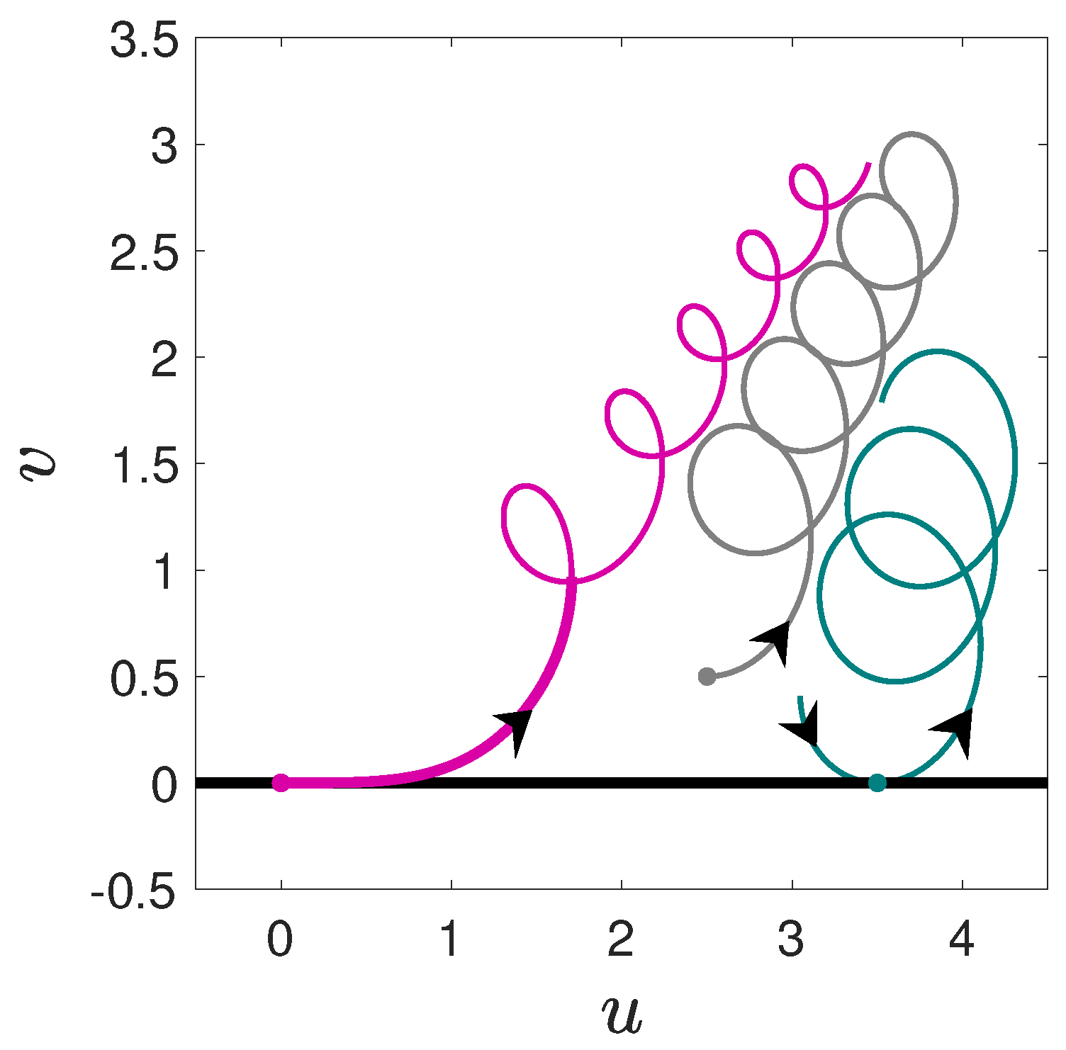
Figure 1. Locally at the nucleus this trajectory corresponds to the trajectory used to define the Poincaré return map in the parallel fields case. As the electron moves away from the nucleus, the electric and magnetic fields create a trajectory that resembles a tapered cycloid with the larger radius closer to the nucleus.
Notice that when projected onto the
-space this trajectory self intersects. Nevertheless, we take the portion of the trajectory shown as bold in
Figure 1 from the nucleus (
) up to the point where the tangent to the trajectory points in the
v direction in
-space. (One could extend the trajectory up to the second time the trajectory passes through the first self-intersection point. However for ease of implementation, we are using a simpler criterion of cutting off the trajectory at the first vertical tangent line.) Next, we replicate this portion of the trajectory into the remaining quadrants in
-space, by first reflecting through the origin and then reflecting about the horizontal axis (See
Figure 2). Reflecting through the origin corresponds to launching a trajectory from the nucleus along the
u-axis to the left. On the other hand, reflecting about the
u-axis is equivalent to time reversal giving two trajectories that move toward the nucleus. In
Figure 2, we show portions of the trajectories launched away from the nucleus in blue, and the time-reversed partners in red. We call these the SOS curves. The arrows denote the direction of time along the trajectory. Thus, a trajectory comes in towards the nucleus from the upper left and continues smoothly into the trajectory in the upper right. Similarly a trajectory comes in from the lower right and exits on the lower left. These two trajectories are analogous to trajectories moving either left or right along the
u-axis in the parallel fields case. In the parallel fields case these trajectories lie on top of one another, whereas here the vector potential splits them into separate curves.
The SOS is now defined by recording the electron’s position and momentum whenever an electron trajectory intersects either the red or the blue curves while moving from the region labeled 1 to the region labeled 2. We do not consider crossings from region 2 to region 1 as part of the SOS. Thus we only consider upward propagating trajectories on the lower right and downward propagating trajectories on the upper right. For the parallel fields problem these two branches were identified, but this is no longer possible in the crossed fields case due to the broken time-reversal symmetry. Nevertheless, the picture can be simplified by taking advantage of another symmetry. There remains a reflection symmetry through the origin in which the upper left branch is identified with the lower right branch, and the lower left branch is identified with the upper right branch. We therefore compose the SOS from just the two branches on the right.
This definition of the SOS is free of tangencies for any trajectory approaching from region 1. This is because the curve that defines the SOS is a portion of a physical trajectory. To show this, suppose a trajectory does intersect the SOS transversely at an isolated point
. Then the direction of the velocity
is determined up to a minus sign at
r. Furthermore, since the trajectory has a fixed energy
E, the magnitude of the velocity at
is determined by setting Equation (
11) equal to zero and solving for
. Thus, the velocity vector
is determined up to a minus sign. If the direction of
coincides with the direction of the trajectory used to define the SOS, then by the uniqueness of the ODE solution, the two trajectories are the same and the intersection
is not an isolated point. Hence, we take
to point in the opposite direction. In this case, the trajectory will curve in the opposite direction as the SOS curve, as shown in
Figure 3. Therefore it intersects the SOS curve coming from region 2. Thus, no trajectory coming from region 1 can intersect the SOS tangentially.
We next introduce canonical coordinates in two-dimensional SOS. We define the position variable a to be the Euclidean length along the SOS trajectory as measured from the nucleus. Positive a parametrizes the curve in the upper right quadrant, and negative a parametrizes the curve in the lower right quadrant. The momentum coordinate is defined by projecting the momentum onto the tangent line to the SOS trajectory.
We now define the Poincaré return map
in the following way. Given
we begin a trajectory at position
a along the SOS trajectory and with the tangential momentum given by
. We determine
by setting Equation (
11) equal to zero. Please note that the tangential component of velocity is given by
, where
is the unit tangent pointing forward along the SOS trajectory (Equation (
9)). Thus, the perpendicular component of velocity is given by
. The sign of
is determined by requiring the normal component of
to point from region 1 to region 2 in
Figure 2. This uniquely determines
, which uniquely determines
via Equation (
9). Now that an initial point
in the full phase space has been determined, we evolve Hamilton’s Equations (
6) forward until the trajectory intersects one of the four branches in
Figure 2 traveling from region 1 into region 2. If the intersection is with one of the two left branches, we reflect the point and its momentum through the origin, i.e.,
. At this point we record the coordinates
on the SOS. Please note that some trajectories will never return to the SOS since the SOS is not globally defined. Such trajectories are easy to identify because they spiral outward toward infinity, escaping the nucleus. See
Figure 1.
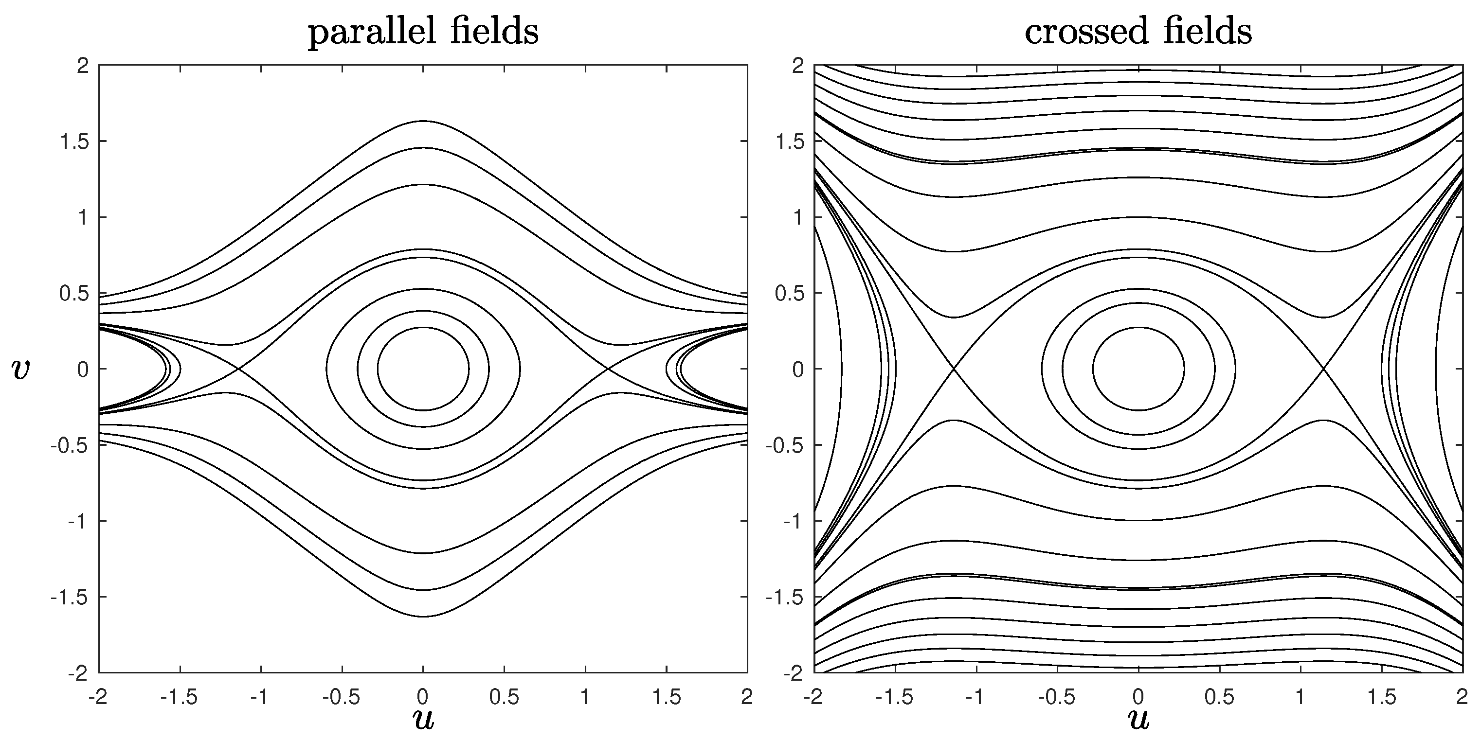
A set of sample SOS plots is shown in
Figure 4. One can notice the presence of periodic orbits and stable islands immersed in the chaotic sea.
4. Visualizing a Periodic Orbit and Its Tangle
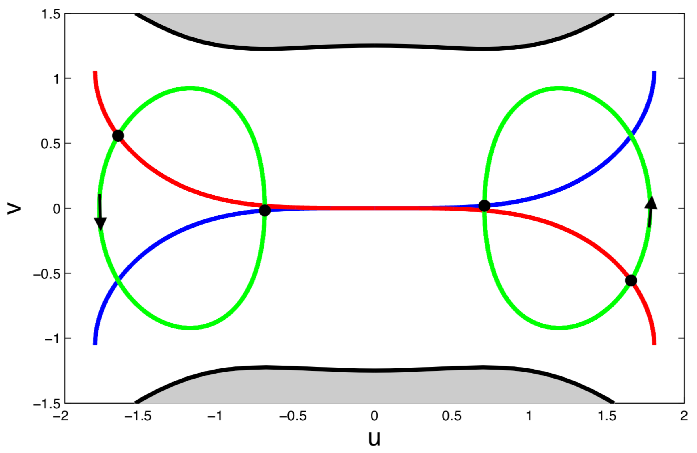
The ionization dynamics of this system is governed by a symmetric pair of periodic orbits in the left and right saddle regions of the potential in
-space. (See
Figure 5) In the original
-coordinates these two periodic orbits are identified into a single orbit near the Stark saddle. In
-space this orbit intersects the SOS curves in four places, but only two of those places intersect the SOS because the orbit must move from region 1 to region 2 as marked with black dots in
Figure 6. These two intersection points form a period-2 orbit of the Poincaré map. This period-2 orbit is hyperbolic.
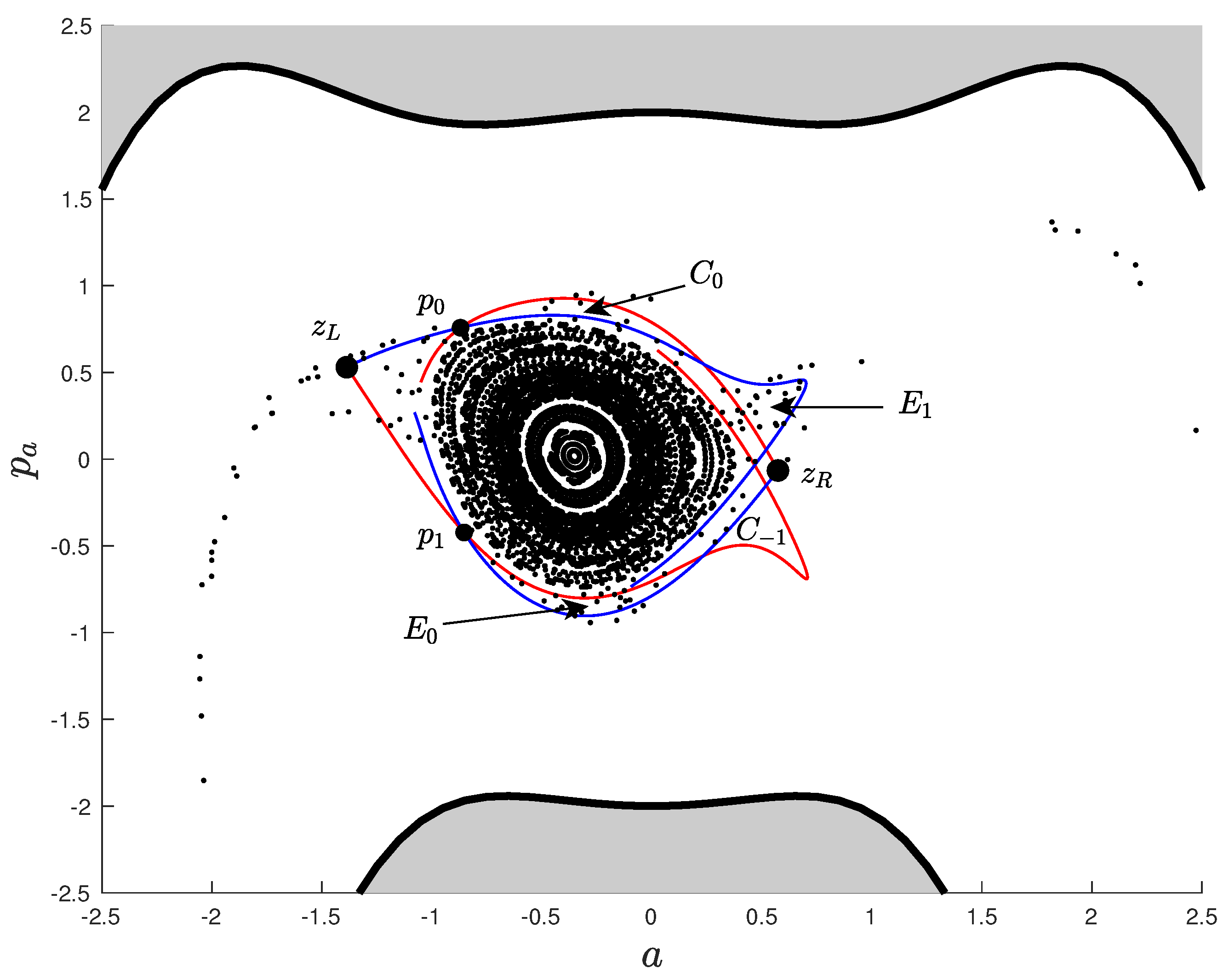
Figure 7 shows a summary of the main results of this paper. The hyperbolic period-2 point has stable and unstable manifolds, shown in red and blue respectively, which intersect to form a heteroclinic tangle. Importantly the SOS for the parameters shown in
Figure 7 is large enough to include not only the period-2 orbit but also the entire resonance zone defined by the tangle. The resonance zone is the domain bounded by the segments of the stable manifold (red) connecting
to
and
to
and by the segments of the unstable manifold (blue) connecting
to
and
to
.
The heteroclinic tangle defines regions in phase space called lobes, which fall into two categories: those governing the escape from the resonance zone, labeled
, and those governing the capture into the resonance zone, labeled
. (See
Figure 7.) The escape lobe
, which is inside the resonance zone, maps to the
lobe, which is outside the resonance zone. Similarly, the capture lobe
, which is outside the resonance zone, maps to the
lobe, which is inside. These lobes define a phase space turnstile which governs the ionization process [
6].
We now return to discuss the issue of tangencies and discontinuities in the Poincaré map. As mentioned before, there are no trajectories that intersect the SOS tangentially coming from region 1. However, in general there may be trajectories that map from the SOS to a tangential intersection with the SOS coming from region 2. See
Figure 3. At any point on the SOS, i.e., at any value of the
a coordinate, these tangential intersections correspond to the minimum value of momentum
. That is, the tangential intersections form the lower black boundary of the physically allowed domain in
Figure 7. Thus, the Poincaré map will be continuous on any topological disk
D that maps forward to a domain that does not intersect the lower boundary of the physically allowed region. It is enough to check just the boundary of the domain
D. That is, if the boundary of a domain
D maps forward to a closed curve that does not intersect the lower boundary of the physically allowed region, then the Poincaré map is continuous over the entire domain
D. The resonance zone of the tangle in
Figure 7 satisfies this property, and thus the Poincaré map is continuous over the entire resonance zone. The same argument applies to the inverse Poincaré map.
To complete the picture, we have also included additional orbits (represented by black dots) that are contained inside the heteroclinic tangle. One can observe a similar prominent chain of stable islands contained inside this heteroclinic tangle as the one shown in
Figure 4. It is important to note that it is the heteroclinic tangle attached to the periodic orbit furthest away from the nucleus that governs the ionization process. Any additional heteroclinic tangles that might exist in the system would be contained inside this outermost tangle.
As we have mentioned earlier, this SOS is not defined globally. For any given set of parameter values, there are always trajectories that do not return to the SOS. For some set of parameter values, the SOS is large enough to encompass the whole of the resonance zone of the heteroclinic tangle. However, this does not hold for all parameter values but only for a certain range of magnetic field strength and energy. Two opposing effects determine the range of validity: the Euclidean distance from the nucleus where the trajectory has its first vertical tangent when projected to the
-space, and the position of the unstable periodic orbit. For a fixed value of electron energy increasing the magnetic field decreases the Larmor radius of the SOS trajectory we use to define the Poincaré SOS and hence decreases the range of the
a coordinate in the local SOS. At the same time the unstable period-two orbit moves away from the nucleus, and hence it its
a coordinate increases, until it finally “slips off” the SOS.
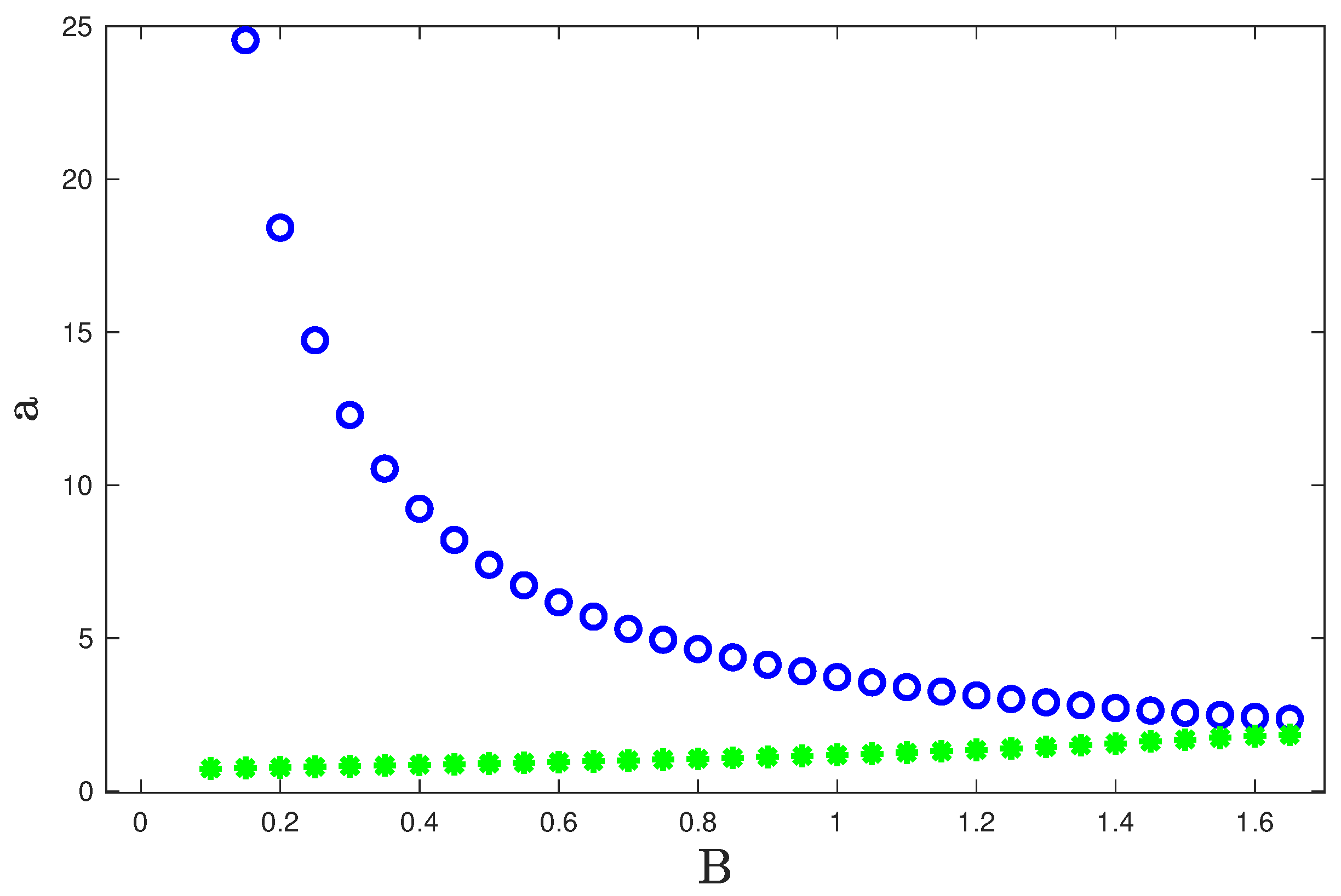
Figure 8 shows the
B-dependance of the position of the periodic orbit and the edge of the SOS definition. For a critical value of the magnetic field strength, the periodic orbit falls off the surface of section, and this ceases to be a useful local SOS for representing the heteroclinic tangle structure. This happens at the value of B for which the blue and the green curves meet in
Figure 8. (For
this failure occurs at
.)
Since the portion of phase space that has been promoted from bound to ionized via a turnstile never returns to the bound state, we argue that the local SOS is sufficient if one is interested in studying the chaotic ionization mechanism in this system.


