Global Analysis and Optimal Control of a Periodic Visceral Leishmaniasis Model

Abstract

In this paper, we propose and analyze a mathematical model for the dynamics of visceral leishmaniasis with seasonality. Our results show that the disease-free equilibrium is globally asymptotically stable under certain conditions when ${\mathcal{R}}_0$, the basic reproduction number, is less than unity. When ${\mathcal{R}}_0>1$ and under some conditions, then our system has a unique positive $\omega$-periodic solution that is globally asymptotically stable. Applying two controls, vaccination and treatment, to our model forces the system to be non-periodic, and all fractions of infected populations settle on a very low level.

1. Introduction

Leishmaniasis is a vector borne, zoonotic disease transmitted to humans and animals through the bite of infected phlebotomine sandflies. The World Health Organization considers leishmaniasis as the sixth most important endemic disease in the world because it has the second-highest number of affected people after malaria and causes an important public health problem in several countries around the world [1].

Leishmaniaisis has many forms, the most important being cutaneous leishmaniasis and visceral leishmaniasis. The cutaneous form is rarely fatal, but it can lead to tissue destruction, scarring, and serious visible impairment. These can lead to social stigmas because of the deformation of the face with permanent scarring. The visceral form, which is almost 100% fatal if left untreated, requires a lengthy and very costly treatment that should be taken under medical supervision [2]. In some cases, depending on the immunity, after the treatment of visceral leishmaniasis, another form of the disease may develop, the post-kala-azar dermal leishmaniasis (PKDL) form, which is not a fatal form; most cases will self-cure, but severe and chronic cases must be treated, and it plays an important role for the dynamics of the disease as it acts as a reservoir for the parasite [3]. Naturally, a time delay could be inserted for PKDL development, as this would make the mathematics very rich and interesting.

Leishmaniasis is distributed in around 90 countries of the world, most of which are developing countries, and more than 90% of the cases are found in India, Nepal, Iran, Iraq and Sudan; there are approximately 350 million people at risk of leishmaniasis in these areas [4]. Leishmaniasis is very hard to control, because it can be transmitted to many mammals, which play the role of a reservoir to the disease, and the transmission to humans can be restarted at any time, causing a high prevalence of the disease even after a long period of no disease or low prevalence of the disease.

Some studies have suggested that there is a correlation between seasonal variations and the abundance of sandflies, which leads to a link between seasonal variations and the prevalence of the disease [5,6,7,8,9,10]. Tiwary et al. [9] found that sandflies are highly prevalent in the rainy season and that the lowest rate of infection with visceral leishmaniasis was observed in the rainy season. This might be due to the flushing effect of rainfall on immature, emerging sandflies. Turki et al. [10] found that the increase in temperature during summer can lead to an increase of cutaneous leishmaniasis cases. They also found an indication that rainfall has no impact or influence on the species of sandflies in the highlands; however, they found that in the lowlands, increased rainfall can lead to increased numbers of cases of cutaneous leishmaniasis, except during the winter season. There is not yet a vaccine for visceral leishmaniasis; however, this is biologically feasible, as many people before the age of vaccinology use a procedure called leishmanization to protect themselves from the infection. Leishmanization procedure is the process of introducing a live but weak form of the parasite to stimulate immune response in order protect from the real infection [11].

Some mathematical models have been developed to study the dynamics of visceral and cutaneous leishmanaisis. Dye [12] designed a mathematical model for the dynamics of zoonotic visceral leishmaniasis, and his model also focused on the dynamics of infection in dogs. His results show that insecticides are the most effective control method; the second-best strategy is to reduce susceptibility to leishmaniasis by vaccinating people or dogs, or by eliminating childhood malnutrition where it is common. Both killing vectors and reducing susceptibility (by whatever means) are more effective than killing dogs or treating them with drugs. Dye et al. [13] formulated an age-structured mathematical model to investigate the effects of visceral leishmaniasis on children, as well as the correlation between malnutrition and the susceptibility of leishmaniasis. His model consists of a system of partial differential equations for the human population, but it has no equation for the animal reservoir nor for the vector reservoir. Lysenko et al. [14] developed an epidemic model for the transmission of cutaneous leishmaniasis. However, the mechanisms that govern the dynamics of the transmission of leishmania parasites are not explicitly stated; therefore, no control strategies for the disease can be proposed. Recently, Rabinovich et al. [15] added some realism to this model by making the probability of developing cutaneous lesions a function of the number of infective bites by sandflies. Burattini et al. [16] formulated a mathematical model to describe the dynamics of the transmission of leishmaniasis, including populations of vector, human and animal (dogs) hosts. Assuming that all populations are both sources and sinks of leishmania parasites, they estimated R0: the infection persistence threshold condition from the sum of individual terms for transmission in humans and in dogs. However, their model did not include the role of PKDL humans in the disease transmission, who have a major role, as PKDL humans act as a source of infection for vectors [17]. Chaves et al. [1] developed a mathematical model for the American cutaneous leishmaniasis. Their model describes the transmission of American cutaneous leishmaniasis in three different populations, a human host population, an animal reservoir population and a vector population, but they considered humans as sinks of the infection only; hence humans in their model are not a source of infection for the vectors.

Elmojtaba et al. [18] developed a mathematical model to understand the dynamics of visceral leishamniasis and determined the local and global stability of the disease-free equilibrium, as well as the local stability of the endemic equilibrium. Elmojtaba et al. [19] developed a model to study the role of cross-immunity between two different strains of leishmaniasis in the eradication of the disease; Elmojtaba et al. [20] also studied the dynamics of malaria and leishmaniasis co-infection to set up some control measures against the spread of these two diseases. Elmojtaba et al. [21] studied the role of infected immigrants and vaccination on the dynamics of visceral leishmaniasis under these settings. All these models used the same assumptions with constant coefficients; however, here in this paper, we consider a model with periodic coefficients.

This paper is organized as follows: the first section gives an introduction for the topic; in the second section, the model is built; the third section gives an intensive mathematical analysis of the model; the optimal control problem is proposed and analyzed in the fourth section; numerical simulations have been carried out and are presented in the fifth section; and a discussion is given in the last section.

2. Model Formulation

To formulate this model, we follow Elmojtaba et al. [18], and we consider the transmission of the disease between three different populations, a human host population, $N_H(t)$; a reservoir host population, $N_R(t)$; and a vector population, $N_V(t)$. We let the human host population be divided into four categories, susceptible individuals, $S_H(t)$; those who are infected with visceral leishmaniasis, $I_H(t)$; those who develop PKDL after the treatment of visceral leishmaniasis, $P_H(t)$; and those who are recovered and have permanent immunity, $R_H(t)$. This implies that

$$N_H(t)=S_H(t)+I_H(t)+P_H(t)+R_H(t)$$

Similarly, we let the reservoir host population be divided into two categories, a susceptible reservoir $S_R(t)$, and an infected reservoir $I_R(t)$, such that

$$N_R(t)=S_R(t)+I_R(t)$$

We let the vector population have two categories, susceptiblesandflies $S_V(t)$, and infected sandflies $I_V(t)$, such that

$$N_V(t)=S_V(t)+I_V(t)$$

It is assumed that susceptible individuals are recruited into the population at a constant rate ${\mathrm{\Lambda }}_H$ and acquire infection with leishmaniasis following contact with infected sandflies at a per capita rate $a(t)b\frac{I_V}{N_H}$, where $a(t)$ is the per capita biting rate of sandflies on humans (or reservoirs) and b is the transmission probability per bite per human. The per capita biting rate of sandflies a is equal to the number of bites received per human from sandflies due to conservation of bites mechanism. Infected humans die as a result of leishmaniasis at an average rate $\delta$ or receive treatment at an average rate ${\alpha }_1$; a fraction $\sigma$ of those that are treated recover and acquire permanent immunity, and a fraction $(1-\sigma )$ develop PKDL. Humans with PKDL are treated at an average rate ${\alpha }_2$ or recover naturally at an average rate $\beta$; they acquire permanent immunity in both cases. There is a per capita natural mortality rate ${\mu }_h$ in all human subpopulations.

Susceptible reservoirs are recruited into the population at a constant rate ${\mathrm{\Lambda }}_R$ and acquire infection with leishmaniasis following contact with infected sandflies at a rate $a(t)b\frac{I_V}{N_H}$, where $a(t)$ and b are as described above. We assume that the transmission probability per bite is the same for human and the reservoir because sandflies do not distinguish between humans and reservoirs. It is also assumed that reservoirs do not die as a result of the disease, but a per capita natural mortality rate ${\mu }_r$ occurs in the reservoir population.

Susceptible sandflies are recruited at a constant rate ${\mathrm{\Lambda }}_V$ and acquire leishmaniasis infection following contact with humans infected with leishmaniasis or having PKDL, or reservoirs infected with leishmaniasis, at an average rate equal to $a(t)c\frac{I_H}{N_H}+a(t)c\frac{P_H}{N_H}+a(t)c\frac{I_R}{N_R}$, where $a(t)$ is the per capita biting rate and c is the transmission probability for sandfly infection. Sandflies suffer natural mortality at a per capita rate ${\mu }_v$ regardless of their infection status.

We assume that $a(t)$ (the per capita biting rate of sandflies on humans) is a time-dependent $\omega$-periodic function. With this assumption and the description of the terms, we obtain the following system of differential equations:

$$\begin{array}{ccc}\hfill S_H^{\prime }& =& {\mathrm{\Lambda }}_H-a(t)b{I}_V\frac{S_H}{N_H}-{\mu }_h{S}_H\hfill \\ \hfill I_H^{\prime }& =& a(t)b{I}_V\frac{S_H}{N_H}-({\alpha }_1+\delta +{\mu }_h)I_H\hfill \\ \hfill P_H^{\prime }& =& (1-\sigma ){\alpha }_1{I}_H-({\alpha }_2+\beta +{\mu }_h)P_H\hfill \\ \hfill R_H^{\prime }& =& \sigma {\alpha }_1{I}_H+({\alpha }_2+\beta )P_H-{\mu }_h{R}_H\hfill \\ \hfill S_R^{\prime }& =& {\mathrm{\Lambda }}_R-a(t)b{I}_V\frac{S_R}{N_R}-{\mu }_r{S}_R\hfill \\ \hfill I_R^{\prime }& =& a(t)b{I}_V\frac{S_R}{N_R}-{\mu }_r{I}_R\hfill \\ \hfill S_V^{\prime }& =& {\mathrm{\Lambda }}_V-a(t)c{S}_V\frac{I_H}{N_H}-a(t)c{S}_V\frac{P_H}{N_H}-a(t)c{S}_V\frac{I_R}{N_R}-{\mu }_v{S}_V\hfill \\ \hfill I_V^{\prime }& =& a(t)c{S}_V\frac{I_H}{N_H}+a(t)c{S}_V\frac{P_H}{N_H}+a(t)c{S}_V\frac{I_R}{N_R}-{\mu }_v{I}_V\hfill \end{array}$$

(1)

with

$$\begin{array}{ccc}\hfill N_H^{\prime }& =& {\mathrm{\Lambda }}_H-{\mu }_h{N}_H-\delta I_H\hfill \\ \hfill N_R^{\prime }& =& {\mathrm{\Lambda }}_R-{\mu }_r{N}_R\hfill \\ \hfill N_V^{\prime }& =& {\mathrm{\Lambda }}_V-{\mu }_v{N}_V\hfill \end{array}$$

Invariant Region

All parameters of the model are assumed to be non-negative; furthermore, because Equation (1) monitors living populations, it is assumed that all the state variables are non-negative at time $t=0$. It is noted that in the absence of the disease $(\delta =0)$, the total human population size $N_H\to {\mathrm{\Lambda }}_H/{\mu }_h$ as $t\to \infty$; additionally, $N_R\to {\mathrm{\Lambda }}_R/{\mu }_r$ and $N_V\to {\mathrm{\Lambda }}_V/{\mu }_v$ as $t\to \infty$. This shows that the biologically feasible region

$\mathsf{\Omega }=\{(S_H,I_H,P_H,R_H,S_R,I_R,S_V,I_V)\in R_{+}^8:S_H,I_H,P_H,R_H,S_R,I_R,S_V,I_V\ge 0,$ $N_H\le \frac{{\mathrm{\Lambda }}_H}{{\mu }_h}$, $N_R\le \frac{{\mathrm{\Lambda }}_R}{{\mu }_r},$ $N_V\le \frac{{\mathrm{\Lambda }}_V}{{\mu }_v}\}$ is a positively invariant domain, and thus the model is epidemiologically and mathematically well posed; it is sufficient to consider the dynamics of the flow generated by Equation (1) in this positively invariant domain $\mathsf{\Omega }$.

3. Analysis of the Model

In this section, we analyze Equation (1) to obtain the equilibrium points of the system and their stability. We consider the equations for the proportions by first scaling the subpopulations $N_H$, $N_R$ and $N_V$ using the following set of new variables:

$${\displaystyle s_h=\frac{{\displaystyle S_H}}{{\displaystyle N_H}},i_h=\frac{{\displaystyle I_H}}{{\displaystyle N_H}},p_h=\frac{{\displaystyle P_H}}{{\displaystyle N_H}},r_h=\frac{{\displaystyle R_H}}{{\displaystyle N_H}},s_r=\frac{{\displaystyle S_R}}{{\displaystyle N_R}},i_r=\frac{{\displaystyle I_R}}{{\displaystyle N_R}},s_v=\frac{{\displaystyle S_V}}{{\displaystyle N_V}},\mathrm{and}{i}_v=\frac{{\displaystyle I_V}}{{\displaystyle N_V}}}$$

and let $m=\frac{N_V}{N_H}$ be the female vector–human ratio defined as the number of female sandflies per human host [18]. We note that the ratio m is taken as a constant because it is well known that a vector takes a fixed number of blood meals per unit time independent of the population density of the host. Similarly, we let $n=\frac{N_V}{N_R}$ be the female vector–reservoir ratio defined as the number of female sandflies per reservoir host.

Differentiating with respect to time t and simplifying gives the following reduced system of differential equations:

$$\begin{array}{ccc}\frac{d{s}_h}{dt}\hfill & =\hfill & {\displaystyle \frac{{\mathrm{\Lambda }}_H}{N_H}-[a(t)bm{i}_v+\frac{{\mathrm{\Lambda }}_H}{N_H}-\delta i_h]s_h}\hfill \\ \frac{d{i}_h}{dt}\hfill & =& {\displaystyle a(t)bm{i}_v{s}_h-[{\alpha }_1+\delta +\frac{{\mathrm{\Lambda }}_H}{N_H}-\delta i_h]i_h}\hfill \\ \frac{d{p}_h}{dt}\hfill & =& a(t)bm{i}_v{s}_h-[{\alpha }_2+\beta +\frac{{\mathrm{\Lambda }}_H}{N_H}-\delta i_h]p_h\hfill \\ \frac{d{r}_h}{dt}\hfill & =& \sigma {\alpha }_1{i}_h+[{\alpha }_2+\beta ]p_h-[\frac{{\mathrm{\Lambda }}_H}{N_H}-\delta i_h]r_h\hfill \\ \frac{d{s}_r}{dt}\hfill & =& \frac{{\mathrm{\Lambda }}_R}{N_R}-a(t)bn{i}_v{s}_r-\frac{{\mathrm{\Lambda }}_H}{N_H}{s}_r\hfill \\ \frac{d{i}_r}{dt}\hfill & =& a(t)bn{i}_v{s}_r-\frac{{\mathrm{\Lambda }}_H}{N_H}{i}_r\hfill \\ \frac{d{s}_v}{dt}\hfill & =& \frac{{\mathrm{\Lambda }}_V}{N_V}-[a(t)c{i}_h+a(t)c{p}_h+a(t)c{i}_r+\frac{{\mathrm{\Lambda }}_V}{N_V}]s_v\hfill \\ \frac{d{i}_v}{dt}\hfill & =& [a(t)c{i}_h+a(t)c{p}_h+a(t)c{i}_r]s_v-\frac{{\mathrm{\Lambda }}_V}{N_V}{i}_v\hfill \end{array}$$

(2)

3.1. Mathematical Properties

We let C denote all continuous functions on the real line. Given $f\in C$, and if f is $\omega$-periodic, then the average value of f on a time interval [0,$\omega$] can be defined as

$$\overline{f}=\frac{1}{\omega }{\int }_0^{\omega }f(t)\mathrm{d}t$$

The maximum and minimum values of f on a time interval [0,$\omega$] are denoted as $f^M$ and $f^m$, respectively, and are defined as

$$f^M=\underset{t\in [0,\omega ]}{max}f(t)$$

and

$$f^m=\underset{t\in [0,\omega ]}{min}f(t)$$

Then the following result is valid:

Proposition 1.

Every forward solution of Equation (2) in ${\mathbb{R}}_{+}^8$ eventually enters into the closed set $\mathsf{\Omega }=\{(s_h,i_h,p_h,r_h,s_r,i_r,s_v,i_v)\in {\mathbb{R}}_{+}^8:0\le s_h,i_h,p_h,r_h,s_h+i_h+p_h+r_h\le 1,0\le s_r,i_r,s_r+i_r\le 1,0\le s_v,i_v,s_v+i_v\le 1\}$ and Ω is positively invariant.

This proposition shows that the scaled system (Equation (2) is epidemiologically and mathematically well-posed, and it is sufficient to consider the dynamics of the flow generated by Equation (2) in this positively invariant domain $\mathsf{\Omega }$. Here ${\mathbb{R}}_{+}^8$ denotes the non-negative cone of ${\mathbb{R}}^8$ including its lower-dimensional faces. We denote the boundary and the interior of $\mathsf{\Omega }$ by $\mathsf{\partial }\mathsf{\Omega }$ and $\stackrel{\circ }{\mathsf{\Omega }},$ respectively.

Proof. 

The proof is straightforward. ☐

3.2. Global Stability of the Disease-Free Equilibrium

It is clear that the system given by Equation (2) admits a unique disease-free equilibrium $E_0=(1,0,0,0,1,0,1,0)$.

We let $({\mathbb{R}}^n,{\mathbb{R}}_{+}^n)$ be an ordered n-dimensional Euclidean space with a norm $\left|\right|.\left|\right|$, and we assume that int$({\mathbb{R}}_{+}^n)\ne \varnothing$. We let x, y∈${\mathbb{R}}^n$, and we say $x⩾y$ if $x-y\in {\mathbb{R}}_{+}^n$, $x>y$ if $x-y\in {\mathbb{R}}_{+}^n⧹\left\{0\right\}$ and $x\gg y$ if $x-y\in$ int $({\mathbb{R}}_{+}^n)$.

The following lemma will be useful for proving global stability of $E_0$.

Lemma 1.

(Lemma 2.1 in [22]). Let $A(t)$ be a continuous, cooperative, irreducible, and ω-periodic $n\times n$ matrix function. Let ${\mathsf{\Phi }}_{A(.)}(t)$ be the fundamental matrix of the linear non-autonomous differential equation $\dot{x}=A(t)x$, where x is a $n\times 1$ vector. Let $\mu =\frac{1}{\omega }lnr({\mathsf{\Phi }}_{A(.)}(\omega ))$, where $r({\mathsf{\Phi }}_{A(.)}(\omega ))$ is the spectral radius of the monodromy matrix ${\mathsf{\Phi }}_{A(.)}(\omega )$. Then there exists a positive ω-periodic function $v(t)$ such that $e^{\mu t}v(t)$ is a solution of $\dot{x}=A(t)x$.

Now let $x={(i_h,p_h,i_r,i_v)}^T$, $\mathcal{F}(t,x)$ denotes the new infection rate and $\mathcal{V}(t,x)$ denotes the rate of transfer of individuals between infection compartment; therefore the vectors $\mathcal{F}(t,x)$ and $\mathcal{V}(t,x)$ given by

$$\begin{array}{c}\hfill \mathcal{F}(t,x)=\left[\begin{array}{c}a(t)bm{i}_v{s}_h\\ 0\\ a(t)bn{i}_v{s}_r\\ (a(t)c{i}_h+a(t)c{p}_h+a(t)c{i}_r)s_v\end{array}\right],\mathcal{V}(t,x)=\left[\begin{array}{c}({\alpha }_1+\delta +\frac{{\mathrm{\Lambda }}_H}{N_H}-\delta i_h)i_h\\ ({\alpha }_2+\beta +\frac{{\mathrm{\Lambda }}_H}{N_H}-\delta i_h)p_h-(1-\sigma ){\alpha }_1{i}_h\\ \frac{{\mathrm{\Lambda }}_R}{N_R}{i}_r\\ \frac{{\mathrm{\Lambda }}_V}{N_V}{i}_v\end{array}\right]\end{array}$$

Therefore, see [23], $F(t)$ and $V(t)$ given by

$${\displaystyle F(t)={\left(\frac{\mathsf{\partial }{\mathcal{F}}_i(t,E_0)}{\mathsf{\partial }{x}_j}\right)}_{1⩽i,j⩽4}=\left(\begin{array}{cccc}0& 0& 0& a(t)bm\\ 0& 0& 0& 0\\ 0& 0& 0& a(t)bn\\ a(t)c& a(t)c& a(t)c& 0\end{array}\right)}$$

and

$${\displaystyle V(t)={\left(\frac{\mathsf{\partial }{\mathcal{V}}_i(t,E_0)}{\mathsf{\partial }{x}_j}\right)}_{1⩽i,j⩽4}=\left(\begin{array}{cccc}{\alpha }_1+\delta +{\mu }_h& 0& 0& 0\\ -(1-\sigma ){\alpha }_1& {\alpha }_2+\beta +{\mu }_h& 0& 0\\ 0& 0& {\mu }_r& 0\\ 0& 0& 0& {\mu }_v\end{array}\right)}$$

Now, $F(t)$ is non-negative and $-V(t)$ is co-operative (off-diagonal elements are non-negative). Thus, $F(t)-V(t)$ is continuous and co-operative and irreducible. Therefore, Lemma 1 is applicable to the system $\dot{X}=(F(t)-V(t))X$, where $X={(i_h,p_h,i_r,i_v)}^T$.

The following result will hold:

Proposition 2.

If $r({\mathsf{\Phi }}_{F(.)-V(.)}(\omega ))<1$ then the disease-free equilibrium $E_0$ is globally asymptotically stable.

Proof. 

From the system given by Equation (2), we have the system of equations:

$$\begin{array}{c}\hfill \begin{array}{ccc}{i}_h^{\prime }\hfill & =\hfill & a(t)bm{i}_v{s}_h-\left[{\alpha }_1+\delta +\frac{{\mathrm{\Lambda }}_H}{N_H}-\delta i_h\right]i_h\hfill \\ p_h^{\prime }\hfill & =\hfill & (1-\sigma ){\alpha }_1{i}_h-\left[{\alpha }_2+\beta +\frac{{\mathrm{\Lambda }}_H}{N_H}-\delta i_h\right]p_h\hfill \\ i_r^{\prime }\hfill & =\hfill & a(t)bn{i}_v{s}_r-\frac{{\mathrm{\Lambda }}_H}{N_H}{i}_r\hfill \\ i_v^{\prime }\hfill & =\hfill & a(t)c{i}_h{s}_v+a(t)c{p}_h{s}_v+a(t)c{i}_r{s}_v-\frac{{\mathrm{\Lambda }}_V}{N_V}{i}_v\hfill \end{array}\end{array}$$

We observe that

$$\frac{d}{dt}{[i_h,p_h,i_r,i_v]}^T⩽[F(t)-V(t)]{[i_h,p_h,i_r,i_v]}^T$$

Now, we consider the linear auxiliary system:

$$\frac{dX}{dt}=[F(t)-V(t)]X$$

(3)

Applying Lemma 1 there exists an $\omega$-periodic function $\overline{X}(t)$ such that $X(t)=e^{st}\overline{X}(t)$ is a solution of the system given by Equation (3), where $s=\frac{1}{\omega }ln\left[r({\mathsf{\Phi }}_{F(.)-V(.)}(\omega ))\right]$.

Now, by the comparison principle [24], for any $[i_h(0),p_h(0),i_r(0),i_v(0)]⩽MX(0)$ and for some sufficiently large $M>0$, we have $[i_h,p_h,i_r,i_v]⩽MX(t)$. Because $r({\mathsf{\Phi }}_{F(.)-V(.)}(\omega ))<1$, therefore, $X(t)\to 0$ as $t\to \infty$. Thus, $i_h(t)\to 0$, $p_h(t)\to 0$, $i_r(t)\to 0$ and $i_v(t)\to 0$ as $t\to \infty$.

Using the theory of asymptomatic autonomous systems [25], we have $r_h(t)\to 0$, $s_h(t)\to 1$, $s_r(t)\to 1$, and $s_v(t)\to 1$ as $t\to \infty$.

Thus, $E_0=(1,0,0,0,1,0,1,0)$ is globally asymptotically stable if $r({\mathsf{\Phi }}_{F(.)-V(.)}(\omega ))<1$. ☐

3.3. Basic Reproduction Number

We let, for each $s\in \mathbb{R}$, the $4\times 4$ matrix $Y(t,s),\forall t⩾s$ satisfy the $\omega$-periodic system:

$$\frac{dy}{dt}=-V(t)y$$

(4)

and $Y(s,s)=I$, where I is the $4\times 4$ identity matrix.

We let $C_{\omega }$ be the ordered Banach space of all $\omega$-periodic functions from $\mathbb{R}$ to ${\mathbb{R}}^4$, which is equipped with maximum norm $\left|\right|.\left|\right|$ and the positive cone $C_{\omega }^{+}=\{\varphi \in C_{\omega }:\varphi (t)⩾0,\forall t\in \mathbb{R}\}$. We define the linear operator $L:C_{\omega }\to C_{\omega }$ as follows:

$${\displaystyle (L\varphi )(t)={\int }_0^{\infty }Y(t,t-a)F(t-a)\varphi (t-a)\mathrm{d}a,\forall t\in \mathbb{R},\varphi \in C_{\omega }}$$

(5)

The definitions of the basic reproduction number ($R_0$) with seasonality in literature was given by [23]. According to the definition, $R_0$ is defined as follows:

$$R_0=r(L)$$

In this paper, we follow the definition of [23] and analyze the model of Equation (2) in terms of the threshold parameter $R_0$.

We use following lemma to infer stability of $E_0$ in terms of $R_0$.

Lemma 2.

(Theorem 2.2 in [23]). The following statements are valid:

1.

$R_0=1$ if and only if $r({\mathsf{\Phi }}_{F(.)-V(.)}(\omega ))=1$.

2.

$R_0>1$ if and only if $r({\mathsf{\Phi }}_{F(.)-V(.)}(\omega ))>1$.

3.

$R_0<1$ if and only if $r({\mathsf{\Phi }}_{F(.)-V(.)}(\omega ))<1$.

Therefore, from Lemma 2 and Proposition 2, we have the following result.

Proposition 3.

If $R_0<1$ then the disease-free equilibrium $E_0$ of the system given by Equation (2) is globally asymptotically stable.

3.4. Existence and Permanence of the Endemic Periodic Solution

In this section, we study the existence and permanence of the endemic periodic state of the model of Equation (2).

Before giving the main result, we give following definitions from [26].

Definition 1.

The system given by Equation (2) is uniformly persistent if ∃ an $\eta >0$ (depending only on parameter values and not on initial conditions) such that for any initial value $(s_h(0),i_h(0),p_h(0),r_h(0),s_r(0),i_r(0),s_v(0),i_v(0))\in {\mathbb{R}}_{+}\times$ int(${\mathbb{R}}_{+}$) × int(${\mathbb{R}}_{+}$) × int(${\mathbb{R}}_{+}$) × ${\mathbb{R}}_{+}$ × int(${\mathbb{R}}_{+}$) × ${\mathbb{R}}_{+}$ × int(${\mathbb{R}}_{+}$) such that every solution $(s_h(t),i_h(t),p_h(t),r_h(t),s_r(t),i_r(t),s_v(t),$ $i-v(t))$ of the system given by Equation (2) satisfies.

${lim}_{t\to \infty }inf{s}_h(t)⩾\eta$, ${lim}_{t\to \infty }inf{i}_h(t)⩾\eta$, ${lim}_{t\to \infty }inf{p}_h(t)⩾\eta$, ${lim}_{t\to \infty }inf{r}_h(t)⩾\eta$, ${lim}_{t\to \infty }inf{s}_r(t)⩾\eta$, ${lim}_{t\to \infty }inf{i}_r(t)⩾\eta$, ${lim}_{t\to \infty }inf{s}_v(t)⩾\eta$, ${lim}_{t\to \infty }inf{i}_v(t)⩾\eta$.

Definition 2.

The system given by Equation (2) is said to be permanent if there exists a compact region ${\mathsf{\Omega }}_0\subset$ int(Ω) such that every solution of the system given by Equation (2) with initial condition $(s_h(0),i_h(0),p_h(0),r_h(0),s_r(0),i_r(0),s_v(0),i_v(0))\in {\mathbb{R}}_{+}\times$ int(${\mathbb{R}}_{+}$) × int(${\mathbb{R}}_{+}$) × int(${\mathbb{R}}_{+}$) × ${\mathbb{R}}_{+}$ × int(${\mathbb{R}}_{+}$) × ${\mathbb{R}}_{+}$ × int(${\mathbb{R}}_{+}$) will eventually enter and remain in the region ${\mathsf{\Omega }}_0$.

A natural concept of dissipation is to assume that there is a bounded set into which every orbit eventually enters and remains [27]. Clearly, for a dissipative dynamical system, proving permanence is equivalent to proving uniform persistence.

We consider the following sets:

$$X={\mathbb{R}}_{+}^8,X_0={\mathbb{R}}_{+}\times int({\mathbb{R}}_{+})\times int({\mathbb{R}}_{+})\times int({\mathbb{R}}_{+})\times {\mathbb{R}}_{+}\times int({\mathbb{R}}_{+})\times {\mathbb{R}}_{+}\times int({\mathbb{R}}_{+}),\mathsf{\partial }{X}_0=X⧹X_0.$$

We let $f:X\to X$ be a continuous map, and we define the following set:

$$M_{\mathsf{\partial }}=\{x\in \mathsf{\partial }{X}_0:f^n(x)\in \mathsf{\partial }{X}_0,n⩾0\}$$

where $f^n$ is the nth iteration of the function.

The following lemma is used to show the uniform persistence of the system given by Equation (2).

Lemma 3.

([26]) Let $W^s(X)$ be the stable set of X. Assume that

1.

$f(X_0)\subseteq X_0$ and f has a global attractor A.

2.

There exists a finite sequence $\mathcal{M}=\{M_1,M_2,\dots .,M_k\}$ of disjoint, compact, and isolated invariant sets in $\mathsf{\partial }{X}_0$ such that

• $\mathsf{\Omega }(M_{\delta })$ = ${\cup }_{x\in M_{\mathsf{\partial }}}\omega (x)\subset {\cup }_{i=1}^k{M}_i$;
• no subset of $\mathcal{M}$ forms a cycle in $\mathsf{\partial }{X}_0$;
• $M_i$ is isolated in X;
• $W^s(M_i)\cap X_0=\varnothing$ for each $1⩽i⩽k$.

Then there exists $\eta >0$ such that $lim{inf}_{n\to \infty }d(f^n(x),\mathsf{\partial }{X}_0)⩾\eta$ for all $x\in X_0$.

We claim the following result:

Proposition 4.

If $R_0>1$ then the solutions of Equation (2) are uniformly persistent, and the system admits at least one positive ω-periodic solution.

Proof. 

Consider the periodic semi-flow $T:{\mathbb{R}}_{+}^8\to {\mathbb{R}}_{+}^8$ associated with Equation (2), defined by

$$T(t)x=u(t,x),\forall x\in {\mathbb{R}}_{+}^8$$

Let $P_1$ be the associated Poincaré map defined as $P_1:=T(\omega )$. We first show that $P_1$ is uniformly persistent with respect to $(X_0,\mathsf{\partial }{X}_0)$.

It is clear that the sets X and $X_0$ are positively invariant for Equation ((2)). Now by Proposition 1, the bounded set $\mathsf{\Omega }$ attracts every solution of Equation (2), and $\mathsf{\Omega }$ is compact. Thus the Poincaré map $P_1$ is point-dissipative and compact on X. Therefore, it follows from Theorem 1.1.3 in [26] that there is a global attractor A of $P_1$ that attracts each bounded set in X.

For Equation (2), the set $M_{\mathsf{\partial }}$ is defined as $M_{\mathsf{\partial }}=\{(s_h(0),i_h(0),p_h(0),r_h(0),s_r(0),i_r(0),s_v(0),$ $i_v(0))\in \mathsf{\partial }{X}_0:$ $P_1^n(s_h(0),i_h(0),p_h(0),r_h(0),s_r(0),i_r(0),s_v(0),i_v(0))\in \mathsf{\partial }{X}_0,\forall n⩾0\}$.

We claim that $M_{\mathsf{\partial }}=\{(s_h,0,0,0,s_r,0,s_v,0):s_h⩾0,s_r⩾0,s_v⩾0\}$. It is clear that $\{(s_h,0,0,0,s_r,0,s_v,0):s_h⩾0,s_r⩾0,s_v⩾0\}\subseteq M_{\mathsf{\partial }}$.

Now, we let $(s_h(0),i_h(0),p_h(0),r_h(0),s_r(0),i_r(0),s_v(0),i_v(0))\in \mathsf{\partial }{X}_0⧹\{(s_h,0,0,0,s_r,0,s_v,0):s_h⩾0,$ $s_r⩾0,$ $s_v⩾0\}$.

If $i_h(0)=0,p_h(0)=0,r_h(0)=0,i_r(0)=0,i_v>0$, then we have $s_h(0)>0,s_r(0)>0,$ $s_v(0)>0,i_v(0)>0.$

From the second equation of the system given by Equation (2), we have.

${\displaystyle i_h^{\prime }(0)>a(t)bm{i}_v(0)s_h(0)>0}$; ${\displaystyle p_h^{\prime }(0)>(1-\sigma ){\alpha }_1{i}_h(0)>0}$; ${\displaystyle r_h^{\prime }(0)>\sigma ){\alpha }_1{i}_h(0)>0}$; ${\displaystyle i_r^{\prime }(0)>a(t)bn{i}_v(0)s_r(0)>0}$; and ${\displaystyle i_v^{\prime }(0)>a(t)c{s}_v(0)(i_h(0)+p_h(0)+i_r(0))>0}$.

Similar holds for other cases also.

Therefore, $(s_h(0),i_h(0),p_h(0),r_h(0),s_r(0),i_r(0),s_v(0),i_v(0))\notin \mathsf{\partial }{X}_0$ for all $0<t\ll 1$. This implies that $M_{\mathsf{\partial }}=\{(s_h,0,0,0,s_r,0,s_v,0):s_h⩾0,s_r⩾0,s_v⩾0\}$.

Now, $P_1$ has a unique fixed point $E_0(s_h,0,0,0,s_r,0,s_v,0)$ in $M_{\mathsf{\partial }}$. It is easy to show that $\left\{E_0\right\}$ is isolated in X and $E_0$ is global attracting in $M_{\mathsf{\partial }}$; therefore we have $\mathsf{\Omega }(M_{\mathsf{\partial }})={\cup }_{x\in M_{\mathsf{\partial }}}\omega (x)\subseteq \left\{E_0\right\}$, where $\omega (x)$ is the omega limit set of x. It is clear that no subset of $\left\{E_0\right\}$ can form a cycle in $\mathsf{\partial }{X}_0$.

Now, we show that $W^s(E_0)\cap X_0=\varnothing$, where $W^s(E_0)$ is the stable set of $E_0$.

We let $x^0=(s_h(0),i_h(0),p_h(0),r_h(0),s_r(0),i_r(0),s_v(0),i_v(0))\in W^s(E_0)\cap X_0$.

Because $x^0\in X_0$, therefore, by the continuity of the solution with respect to the initial conditions we have, for any $ϵ\in (0,1)$, there exists a $\delta >0$ such that $\forall x^0\in X_0$ satisfying $\left|\right|x^0-E_0\left|\right|<\delta$, this implies $\left|\right|u(t,x^0)-u(t,E_0)\left|\right|<ϵ$ $\forall t\in [0,\omega ]$.

We claim that ${lim}_{m\to \infty }sup\left|\right|P_1^m(x^0)-E_0\left|\right|⩾\delta$ $\forall x^0\in X_0$. We suppose, if possible, $\exists x^0\in X_0$ such that ${lim}_{m\to \infty }sup\left|\right|P_1^m(x^0)-E_0\left|\right|<\delta$. Without loss of generality, we can assume that $\left|\right|P_1^m(x^0)-E_0\left|\right|<\delta$ for all $m⩾0$. Therefore, we have $\left|\right|u(t,P_1^m(x^0))-u(t,E_0)\left|\right|<ϵ$, $\forall t\in [0,\omega ]$ and $\forall m⩾0$.

For any $t⩾0$, we let $t=m\omega +t_1$, where $t_1\in [0,\omega ]$ and $m=\left[\frac{t}{\omega }\right]$ is the greatest positive integer less than or equal to $\frac{t}{\omega }$.

Then we have $\left|\right|u(t,P_1^m(x^0))-u(t,E_0)\left|\right|=\left|\right|u(t_1,P_1^m(x^0))-u(t_1,E_0)\left|\right|<ϵ$ for all $t⩾0$.

We let $(s_h(t),i_h(t),p_h(t),r_h(t),s_r(t),i_r(t),s_v(t),i_v(t))=U(t,x^0)$. It follows from the previous argument that $1-ϵ<s_h(t)<1+ϵ$, $1-ϵ<s_r(t)<1+ϵ$, $1-ϵ<s_v(t)<1+ϵ$, $0<i_h(t)<ϵ$, $0<p_r(t)<ϵ$, $0<r_h(t)<ϵ$, $0<i_r(t)<ϵ$, $0<i_v(t)<ϵ$, $\forall t⩾0$.

From Equation (2), we have the following:

$$\begin{array}{c}\hfill \begin{array}{c}\frac{d{i}_h}{dt}⩾a(t)bm{i}_v(1-ϵ)-[{\alpha }_1+\delta +\frac{{\mathrm{\Lambda }}_H}{N_H}-\delta i_h]i_h\hfill \\ \frac{d{p}_h}{dt}⩾(1-\sigma ){\alpha }_1{i}_h-[{\alpha }_2+\beta +\frac{{\mathrm{\Lambda }}_H}{N_H}-\delta i_h]p_h\hfill \\ \frac{d{i}_r}{dt}⩾a(t)bn{i}_v(1-ϵ)-\frac{{\mathrm{\Lambda }}_H}{N_H}{i}_r\hfill \\ \frac{d{i}_v}{dt}⩾a(t)c{i}_h(1-ϵ)+a(t)c{p}_h(1-ϵ)+a(t)c{i}_r(1-ϵ)-\frac{{\mathrm{\Lambda }}_V}{N_V}{i}_v\hfill \end{array}\end{array}$$

(6)

We let ${\displaystyle M_{ϵ}(t)=\left(\begin{array}{cccc}0& 0& 0& a(t)bmϵ\\ 0& 0& 0& 0\\ 0& 0& 0& a(t)bnϵ\\ a(t)cϵ& a(t)cϵ& a(t)cϵ& 0.\end{array}\right)}$

Hence we obtain

$$\frac{d}{dt}{[i_h,p_h,i_r,i_v]}^T⩾[F(t)-V(t)-ϵM_{ϵ}(t)]{[i_h,p_h,i_r,i_v]}^T$$

Now, by Lemma 2, we have that if $R_0>1$, then $r({\mathsf{\Phi }}_{F(.)-V(.)}(\omega ))>1$. We choose $ϵ>0$ sufficiently small so that $r({\mathsf{\Phi }}_{F(.)-V(.)-ϵM_{ϵ}(.)}(\omega ))>1$. Thus by Lemma 1 and the standard comparison theorem [24], ∃ $\omega$-periodic function $f(t)$ such that $x(t)⩾f(t)e^{s_{1}t}$, where $x(t)=[i_h,p_h,i_r,i_v]$ and

$$s_1=\frac{1}{\omega }lnr({\mathsf{\Phi }}_{F(.)-V(.)-ϵM_{ϵ}(.)}(\omega ))>0$$

This implies, as $t\to \infty$, that $i_h(t)\to \infty$, $p_h(t)\to \infty$, $i_r(t)\to \infty$ and $i_v(t)\to \infty$. This is a contradiction, as ${lim}_{t\to \infty }sup\left|\right|P_1^m(x^0)-E_0\left|\right|<\delta$. Therefore, we have ${lim}_{t\to \infty }sup\left|\right|P_1^m(x^0)-E_0\left|\right|⩾\delta$$\forall x^0\in X_0$. This is again impossible, as $x^0\in W^s(E_0)$ (because $x\in W^s(E_0)$ implies ${lim}_{t\to }\infty \left|\right|P_1^m(x^0)-E_0\left|\right|=0$). Thus we have $W^s(E_0)\cap X_0=\varnothing$.

Therefore, by Lemma 3, we have that $P_1$ is uniformly persistent with respect to $(X_0,\mathsf{\partial }{X}_0)$. Therefore, by Theorem 3.1.1 in [26], the periodic semi-flow T is uniformly persistent in X.

Thus, if $R_0>1$, then the solution of the system given by Equation (2) is uniformly persistent.

Now the Poincarè map $P_1$ is point-dissipative and compact, and $P_1$ is also uniformly persistent with respect to $(X_0,\mathsf{\partial }{X}_0)$. Now, $X_0$ is a relatively open set in X and therefore, $\mathsf{\partial }{X}_0$ is a relatively closed set in X. Thus, by Theorem 1.3.6 in [26], $P_1$ has a fixed point $(\overline{s_h}(0),{\overline{i}}_h(0),{\overline{p}}_h(0),\overline{r_h}(0),{\overline{s}}_r(0),{\overline{i}}_r(0),{\overline{s}}_v(0),$ ${\overline{i}}_v(0))\in X_0$. Now we have ${\overline{i}}_h(0)\in$ int$({\mathbb{R}}_{+})$, ${\overline{p}}_h(0)\in$ int$({\mathbb{R}}_{+})$, ${\overline{r}}_h(0)\in$ int$({\mathbb{R}}_{+})$, ${\overline{i}}_r(0)\in$ int$({\mathbb{R}}_{+})$, ${\overline{i}}_v(0)\in$ int$({\mathbb{R}}_{+})$. We need to show that $\overline{s_h}(0)\in$ int$({\mathbb{R}}_{+})$, $\overline{s_r}(0)\in$ int$({\mathbb{R}}_{+})$, $\overline{s_v}(0)\in$ int$({\mathbb{R}}_{+})$. If not, we suppose $\overline{s_h}(0)=0$; then from Equation (2), we have $0=-({\alpha }_1+\delta +\frac{{\mathrm{\Lambda }}_H}{N_H}-\delta \overline{i_h}){\overline{i}}_h(0)\Rightarrow {\overline{i}}_h(0)=0$, a contradiction. Therefore, $\overline{s_h}(0)\in$ int$({\mathbb{R}}_{+})$. Similarly, we can show that $\overline{s_v}(0)\in$ int$({\mathbb{R}}_{+})$ and $\overline{s_r}(0)\in$ int$({\mathbb{R}}_{+})$. Thus,

$$(\overline{s_h}(0),{\overline{i}}_h(0),{\overline{p}}_h(0),\overline{r_h}(0),{\overline{s}}_r(0),{\overline{i}}_r(0),{\overline{s}}_v(0),{\overline{i}}_v(0))\in int({\mathbb{R}}_{+}^8)$$

Therefore,

$$(\overline{s_h}(t),{\overline{i}}_h(t),{\overline{p}}_h(t),\overline{r_h}(t),{\overline{s}}_r(t),{\overline{i}}_r(t),{\overline{s}}_v(t),{\overline{i}}_v(t))=u(t,(\overline{s_h}(0),{\overline{i}}_h(0),{\overline{p}}_h(0),\overline{r_h}(0),{\overline{s}}_r(0),{\overline{i}}_r(0),{\overline{s}}_v(0),{\overline{i}}_v(0)))$$

is the positive $\omega$-periodic solution of the system given by Equation (2). Thus if $R_0>1$, then Equation (2) admits at least one positive periodic solution. ☐

3.5. Global Stability of the Positive Periodic Solution

We claim the following result:

Proposition 5.

If $R_0>1$ and ${\displaystyle \frac{{\mathrm{\Lambda }}_H}{N_H}-4\delta >0}$, then the system given by Equation (2) has a unique positive ω-periodic solution that is globally asymptotically stable.

Proof. 

If $R_0>1$, then we have by Proposition 4 that the system given by Equation (2) admits a positive periodic solution.

We first show that $(\overline{s_h}(t),{\overline{i}}_h(t),{\overline{p}}_h(t),\overline{r_h}(t),{\overline{s}}_r(t),{\overline{i}}_r(t),\overline{s_v}(t),\overline{i_v}(t))$ is globally asymptotically stable if all the conditions of Proposition 5 are satisfied.

We construct the following Lyapunov function: $L(t)=|s_h(t)-\overline{s_h}(t)|+|i_h(t)-{\overline{i}}_h(t)|+|p_h(t)-{\overline{p}}_h(t)|+|r_h(t)-\overline{r_h}(t)|+|s_r(t)-{\overline{s}}_r(t)|+|i_r(t)-{\overline{i}}_r(t)|+|s_v(t)-\overline{s_v}(t)|+|i_v(t)-\overline{i_v}(t)|.$

We use the following formula:

$${\left|x\right|}^{\prime }=sgn(x)x^{\prime }$$

to calculate the upper right-hand derivative (Dini’s derivative) of $L(t)$.

Therefore, we have

$$\begin{array}{c}\hfill \begin{array}{c}{D}^{+}L(t)=sgn|s_h-\overline{s_h}|(-a(t)bm(s_h{i}_v-\overline{s_h}\overline{i_v})-(s_h-\overline{s_h})(\frac{{\mathrm{\Lambda }}_H}{N_H}-\delta (i_h-\overline{i_h})))\hfill \\ +sgn|i_h-\overline{i_h}|(a(t)bm(s_h{i}_v-\overline{s_h}\overline{i_v})-({\alpha }_1+\delta +\frac{{\mathrm{\Lambda }}_H}{N_H}-\delta (i_h-\overline{i_h}))(i_h-\overline{i_h}))\hfill \\ +sgn|p_h-\overline{p_h}|((1-\sigma ){\alpha }_1(i_h-\overline{i_h})-({\alpha }_2+\beta )(p_h-\overline{p_h})-(\frac{{\mathrm{\Lambda }}_H}{N_H}-\delta (i_h-\overline{i_h}))(p_h-\overline{p_h}))\hfill \\ +sgn|r_h-\overline{r_h}|(\sigma {\alpha }_1(i_h-\overline{i_h})+({\alpha }_2+\beta )(p_h-\overline{p_h})-(\frac{{\mathrm{\Lambda }}_H}{N_H}-\delta (i_h-\overline{i_h}))(r_h-\overline{r_h}))\hfill \\ sgn|s_r-\overline{s_r}|(-a(t)bn(i_v{s}_r-\overline{i_v}\overline{s_v})-\frac{{\mathrm{\Lambda }}_R}{N_R}(s_r-\overline{s_r}))\hfill \\ +sgn|i_r-\overline{i_r}|(a(t)bn(i_v{s}_r-\overline{i_v}\overline{s_v})-\frac{{\mathrm{\Lambda }}_R}{N_R}(i_r-\overline{i_r}))\hfill \\ +sgn|s_v-\overline{s_v}|(-a(t)c(s_v{i}_h-\overline{s_v}\overline{i_h})-a(t)c(s_v{p}_h-\overline{s_v}\overline{p_h})-a(t)c(s_v{i}_r-\overline{s_v}\overline{i_r})-\frac{{\mathrm{\Lambda }}_V}{N_V}(s_v-\overline{s_v}))\hfill \\ +sgn|i_v-\overline{i_v}|(a(t)c(s_v{i}_h-\overline{s_v}\overline{i_h})+a(t)c(s_v{p}_h-\overline{s_v}\overline{p_h})+a(t)c(s_v{i}_r-\overline{s_v}\overline{i_r})-\frac{{\mathrm{\Lambda }}_V}{N_V}(i_v-\overline{i_v}))\hfill \\ D^{+}L(t)⩽-|s_h-\overline{s_h}|(\frac{{\mathrm{\Lambda }}_H}{N_H}-\delta )-|i_h-{\overline{i}}_h|(\frac{{\mathrm{\Lambda }}_H}{N_H}-4\delta )\hfill \\ -|p_h-{\overline{p}}_h|(\frac{{\mathrm{\Lambda }}_H}{N_H}-\delta )-|r_h-{\overline{r}}_h|(\frac{{\mathrm{\Lambda }}_H}{N_H}-\delta )-|s_r-{\overline{s}}_r|\frac{{\mathrm{\Lambda }}_H}{N_H}-|i_r-{\overline{i}}_r|\frac{{\mathrm{\Lambda }}_H}{N_H}\hfill \\ -|s_v-{\overline{s}}_v|\frac{{\mathrm{\Lambda }}_V}{N_V}-|i_v-{\overline{i}}_v|\frac{{\mathrm{\Lambda }}_V}{N_V}\hfill \end{array}\end{array}$$

(7)

We let $K=min\{\frac{{\mathrm{\Lambda }}_V}{N_V},\frac{{\mathrm{\Lambda }}_H}{N_H}-4\delta ,\frac{{\mathrm{\Lambda }}_H}{N_H}-\delta \}$. Therefore, $K>0$.

Now,

$$D^{+}L(t)⩽-K\left(|s_h-\overline{s_h}|+|i_h-{\overline{i}}_h|+|p_h-{\overline{p}}_h|+|r_h-{\overline{r}}_h|+|s_r-{\overline{s}}_r|+|i_r-{\overline{i}}_r|+|s_v-{\overline{s}}_v|+|i_v-{\overline{i}}_v|\right)$$

which implies that L is non-increasing on $[0,+\infty )$. Integrating the above inequality from 0 to t, we have

$$\begin{array}{c}\hfill \begin{array}{c}L(t)+K{\int }_0^t(|s_h-\overline{s_h}|+|i_h-{\overline{i}}_h|+|p_h-{\overline{p}}_h|+|r_h-{\overline{r}}_h|\hfill \\ +|s_r-{\overline{s}}_r|+|i_r-{\overline{i}}_r|+|s_v-{\overline{s}}_v|+|i_v-{\overline{i}}_v|)⩽L(0)<\infty ,\forall t⩾0\hfill \end{array}\end{array}$$

(8)

Thus, following Lemma 2.2 in [28], we have ${lim}_{t\to \infty }L(t)=0$. Therefore, it follows that.

${lim}_{t\to \infty }|s_h-\overline{s_h}|=0$, ${lim}_{t\to \infty }|i_h-{\overline{i}}_h|=0$, ${lim}_{t\to \infty }|p_h-{\overline{p}}_h|=0$, ${lim}_{t\to \infty }|r_h-\overline{r_h}|=0$, ${lim}_{t\to \infty }|s_r-{\overline{s}}_r|=0$, ${lim}_{t\to \infty }|i_r-{\overline{i}}_r|=0$, ${lim}_{t\to \infty }|s_v-{\overline{s}}_v|=0$, ${lim}_{t\to \infty }|i_v-{\overline{i}}_v|=0$.

Thus, $(\overline{s_h}(t),{\overline{i}}_h(t),{\overline{p}}_h(t),\overline{r_h}(t),{\overline{s}}_r(t),{\overline{i}}_r(t),\overline{s_v}(t),\overline{i_v}(t))$ is globally asymptotically stable.

Now we show that there exists a unique $\omega$-periodic solution of the system given by Equation (2). For any two $\omega$-periodic solutions $(\overline{s_h}(t),{\overline{i}}_h(t),{\overline{p}}_h(t),\overline{r_h}(t),{\overline{s}}_r(t),{\overline{i}}_r(t),\overline{s_v}(t),\overline{i_v}(t))$ and $(\overline{\overline{s_h}}(t),{\overline{\overline{i}}}_h(t),{\overline{\overline{p}}}_h(t),\overline{\overline{r_h}}(t),{\overline{\overline{s}}}_r(t),{\overline{\overline{i}}}_r(t),\overline{\overline{s_v}}(t),\overline{\overline{i_v}}(t))$ of the system given by Equation (2), we claim that $\overline{s_h}(t)=\overline{\overline{s_h}}(t)$; ${\overline{i}}_h(t)={\overline{\overline{i}}}_h(t)$; ${\overline{p}}_h(t)={\overline{\overline{p}}}_h(t)$ $\overline{r_h}(t)=\overline{\overline{r_h}}(t)$; ${\overline{s}}_r(t)={\overline{\overline{s}}}_r(t)$; ${\overline{i}}_r(t)={\overline{\overline{i}}}_r(t)$; ${\overline{s}}_v(t)={\overline{\overline{s}}}_v(t)$; and ${\overline{i}}_v(t)={\overline{\overline{i}}}_v(t)$, for all $t\in [0,\omega ]$. If not, then there must be at least one $\eta \in [0,\omega ]$ such that $\overline{s_h}(\eta )\ne \overline{\overline{s_h}}(\eta )$, that is, $|\overline{s_h}(\eta )-\overline{\overline{s_h}}(\eta )|=\epsilon >0$.

Thus we can obtain

$$\begin{array}{c}\hfill \begin{array}{ccc}\epsilon \hfill & =\hfill & \underset{n\to \infty }{lim}|\overline{s_h}(\eta +n\varpi )-\overline{\overline{s_h}}(\eta +n\varpi )|\hfill \\ \hfill & =\hfill & \underset{t\to \infty }{lim}|\overline{s_h}(t)-\overline{\overline{s_h}}(t)|>0\hfill \end{array}\end{array}$$

which is contradicting the fact that $(\overline{s_h}(t),{\overline{i}}_h(t),{\overline{p}}_h(t),\overline{r_h}(t),{\overline{s}}_r(t),{\overline{i}}_r(t),\overline{s_v}(t),\overline{i_v}(t))$ is globally asymptotically stable. Therefore $\overline{s_h}(t)=\overline{\overline{s_h}}(t)$, $\forall t\in [0,\omega ]$, and similar holds for other cases also.

Thus if all the conditions of Proposition 5 are satisfied and if $R_0>1$, then the system given by Equation (2) has an unique positive $\omega$-periodic solution that is globally asymptotically stable. ☐

4. The Optimal Control Problem

4.1. Constructing the Problem

We use two different interventions in the model of Equation (1) to reduce the visceral leishmaniasis, namely, vaccination and treatment using antibiotics. The vaccinated population is increased by a proportion $u_1(t){\sigma }_1$ of the susceptible individuals who are successfully vaccinated, where $u_1(t)$ is the per-week vaccination rate and ${\sigma }_1$ is the vaccine efficiency. The vaccinated population is decreased as a result of the waning of vaccine-based immunity (at a rate $ϵ$) to become susceptible again and die (natural deaths) at a rate ${\mu }_h$.

The system of non-linear differential equations representing the effect of different interventions on our basic model from Equation (1) is given as follows:

$$\begin{array}{ccc}\hfill \frac{d{S}_H}{dt}& =& {\mathrm{\Lambda }}_H-a(t)b{I}_V\frac{S_H}{N_H}-({\mu }_h+{\sigma }_1{u}_1)S_H+ϵV\hfill \\ \hfill \frac{d{I}_H}{dt}& =& a(t)b{I}_V\frac{S_H}{N_H}-(u_2+\delta +{\mu }_h)I_H\hfill \\ \hfill \frac{d{P}_H}{dt}& =& (1-\sigma )u_2{I}_H-({\alpha }_2+\beta +{\mu }_h)P_H\hfill \\ \hfill \frac{d{R}_H}{dt}& =& \sigma u_2{I}_H+({\alpha }_2+\beta )P_H-{\mu }_h{R}_H\hfill \\ \hfill \frac{d{V}_H}{dt}& =& {\sigma }_1{u}_1{S}_H-(ϵ+{\mu }_h)V_H\hfill \\ \hfill \frac{d{S}_R}{dt}& =& {\mathrm{\Lambda }}_R-a(t)b{I}_V\frac{S_R}{N_R}-{\mu }_r{S}_R\hfill \\ \hfill \frac{d{I}_R}{dt}& =& a(t)b{I}_V\frac{S_R}{N_R}-{\mu }_r{I}_R\hfill \\ \hfill \frac{d{S}_V}{dt}& =& {\mathrm{\Lambda }}_V-a(t)c{S}_V\frac{I_H}{N_H}-a(t)c{S}_V\frac{P_H}{N_H}-a(t)c{S}_V\frac{I_R}{N_R}-{\mu }_v{S}_V\hfill \\ \hfill \frac{d{I}_V}{dt}& =& a(t)c{S}_V\frac{I_H}{N_H}+a(t)b{S}_V\frac{P_H}{N_H}+a(t)c{S}_V\frac{I_R}{N_R}-{\mu }_v{I}_V\hfill \end{array}$$

(9)

where the initial conditions $S_H(0)$, $I_H(0)$, $P_H(0)$, $R_H(0)$, $V(0)$, $S_R(0)$, $I_R(0)$, $S_V(0)$, and $I_V(0)$ are given, and the definitions of the above model parameters are listed in

Table 1. Parameter values of the model.

Parameter	Value	References
${\mathrm{\Lambda }}_H$	0.0015875 $\times N_h$	[29]
${\mathrm{\Lambda }}_R$	0.0073 $\times N_r$	Assumed
${\mathrm{\Lambda }}_V$	0.299 $\times N_{v_l}$	[30]
${\mu }_h$	0.00004	[31]
${\mu }_r$	0.000274	Assumed
${\mu }_v$	0.189	[30]
b	0.1	Assumed
c	0.0714	[32]
${\alpha }_1$	0.033	[33]
${\alpha }_2$	0.00556	[33]
$1-\sigma$	0.36	[33]
$\delta$	0.011	[34]
$\beta$	0.00556	[33]
$ϵ$	0.02	Assumed

.

The control functions $u_1(t)$ and $u_2(t)$ are bounded and are Lebesgue integrable functions, where the control $u_1(t)$ measures the rate at which susceptible individuals are vaccinated in each time period, and the control $u_2(t)$ represents the effort of treatment of infected individuals.

This performance specification involves the number of infection individuals as well as the cost of applying a vaccination control $(u_1(t))$ and treatment control $(u_2(t))$ in individuals with visceral leishmaniasis. The objective functional to be minimized is defined as

$$J(u_1,u_2)=\underset{0}{\overset{t_f}{\int }}(A{I}_H(t)+\frac{1}{2}C{u}_1^2{\sigma }_1+\frac{1}{2}D{u}_2^2)dt$$

(10)

where $t_f$ is the final time and $A,C$ and D are positive constants to balance the cost factors. The costs can include funds needed for the cost of productive time loss for per premature death, the cost of vaccination per fully immunized person, the cost of vaccination per fully immunized person in high emergencies, the cost for medicine, and hospital admission per case. More often, the cost of implementing a control would be nonlinear. We thus seek to find an optimal control $u_1^{*}(t)$ and $u_2^{*}(t)$ such that

$$J(u_1^{*},u_2^{*})=min\left\{J(u_1,u_2)\right|u_1,u_2\in U\}$$

(11)

where

$$U=\left\{(u_1(t),u_2(t))\right|(u_1(t),u_2(t))\mathrm{measurable},a_i\le (u_1(t),u_2(t))\le b_i,i=1,2,t\in [0,t_1]\}$$

(12)

is the control set.

4.2. Analysis of the Optimal Control Problem

The necessary conditions that an optimal control must satisfy come from Pontryagin’s Maximum Principle [35]. This principle converts the system given by Equation (9) into the problem of minimizing pointwise a Hamiltonian, H, with respect to $u_1$ and $u_2$:

$$H=(A{I}_H(t)+\frac{1}{2}C{u}_1^2{\sigma }_1+\frac{1}{2}D{u}_2^2)+\sum _{i=1}^9{\lambda }_i{g}_i$$

(13)

where $g_i$ is the right-hand side of the differential equation of the ith state variable and ${\lambda }_i$ are the adjoint variables by applying Pontryagin’s Maximum Principle [35,36,37].

Proposition 6.

Given an optimal control $u_1^{*}$ and $u_2^{*}$ and solutions $S_H^{*},I_H^{*},P_H^{*},R_H^{*},V_H^{*},S_R^{*},I_R^{*},S_V^{*},$ and $I_V^{*}$ of the corresponding state system given by Equation (9) that minimizes J($u_1$, $u_2$) over U, then there exists adjoint variables ${\lambda }_i,1\le i\le 9$, satisfying the following:

$$\begin{array}{ccc}\hfill \frac{\mathsf{\partial }{\lambda }_1}{\mathsf{\partial }t}& =& \left[a(t)b\frac{I_V}{N_H}+{\mu }_h+{\sigma }_1{u}_1\right]{\lambda }_1-a(t)b\frac{I_V}{N_H}{\lambda }_2-u_1{\sigma }_1{\lambda }_5\hfill \\ \hfill \frac{\mathsf{\partial }{\lambda }_2}{\mathsf{\partial }t}& =& -A+\left(u_2+\delta +{\mu }_h\right){\lambda }_2-(1-\sigma )u_2{\lambda }_3-\sigma u_2{\lambda }_4+a(t)c\frac{S_V}{N_H}{\lambda }_8-a(t)c\frac{S_V}{N_H}{\lambda }_9\hfill \\ \hfill \frac{\mathsf{\partial }{\lambda }_3}{\mathsf{\partial }t}& =& ({\alpha }_2+\beta +{\mu }_h){\lambda }_3-({\alpha }_2+\beta ){\lambda }_4+a(t)c\frac{S_V}{N_H}{\lambda }_8-a(t)c\frac{S_V}{N_H}{\lambda }_9\hfill \\ \hfill \frac{\mathsf{\partial }{\lambda }_4}{\mathsf{\partial }t}& =& {\mu }_h{\lambda }_4\hfill \\ \hfill \frac{\mathsf{\partial }{\lambda }_5}{\mathsf{\partial }t}& =& (ϵ+{\mu }_h){\lambda }_5+ϵ{\lambda }_1\hfill \\ \hfill \frac{\mathsf{\partial }{\lambda }_6}{\mathsf{\partial }t}& =& \left(a(t)b\frac{I_V}{N_R}+{\mu }_r\right){\lambda }_6-a(t)b\frac{I_V}{N_R}{\lambda }_7\hfill \\ \hfill \frac{\mathsf{\partial }{\lambda }_7}{\mathsf{\partial }t}& =& {\mu }_r{\lambda }_7+a(t)c\frac{S_V}{N_R}{\lambda }_8-a(t)c\frac{S_V}{N_R}{\lambda }_9\hfill \\ \hfill \frac{\mathsf{\partial }{\lambda }_8}{\mathsf{\partial }t}& =& \left(a(t)c\frac{I_H}{N_H}+a(t)c\frac{P_H}{N_H}+a(t)c\frac{I_R}{N_R}+{\mu }_v\right){\lambda }_8-\left(a(t)c\frac{I_H}{N_H}+a(t)c\frac{P_H}{N_H}+a(t)c\frac{I_R}{N_R}\right){\lambda }_9\hfill \\ \hfill \frac{\mathsf{\partial }{\lambda }_9}{\mathsf{\partial }t}& =& a(t)b\frac{S_H}{N_H}{\lambda }_1-a(t)b\frac{S_H}{N_H}{\lambda }_2+a(t)b\frac{S_R}{N_R}{\lambda }_6-a(t)b\frac{S_R}{N_R}{\lambda }_7+{\mu }_v{\lambda }_9\hfill \end{array}$$

(14)

with transversality conditions

$${\lambda }_i(t_f)=0,i=1,.....,9$$

(15)

Furthermore, the control pair ($u_1^{*},u_2^{*}$) is given as

$$\begin{array}{ccc}\hfill u_1^{*}& =& min\left\{b_1,max\left[a_1,\frac{{\sigma }_1({\lambda }_1-{\lambda }_5)S_H}{C{\sigma }_1}\right]\right\}\hfill \\ \hfill and\\ \hfill u_2^{*}& =& min\left\{b_2,max\left[a_2,\frac{({\lambda }_2-(1-\sigma ){\lambda }_3-\sigma {\lambda }_4)I_H}{D}\right]\right\}\hfill \end{array}$$

(16)

Proof. 

The existence of an optimal control is guaranteed using the result by [38]. Thus, the differential equations governing the adjoint variables are obtained by the differentiation of the Hamiltonian function evaluated at the optimal controls, giving the stated adjoint system from Equations (14) and (15).

Furthermore, differentiating the Hamiltonian function with respect to the control variables in the interior of the control set U, where $a_i<u_i<b_i$, $i=1,2$, we have

$$\begin{array}{ccc}\frac{\mathsf{\partial }H}{\mathsf{\partial }{u}_1}\hfill & =\hfill & C{\sigma }_1{u}_1-{\sigma }_1{\lambda }_1{S}_H+{\sigma }_1{\lambda }_5{S}_H=0\hfill \\ \frac{\mathsf{\partial }H}{\mathsf{\partial }{u}_2}\hfill & =\hfill & D{u}_2-{\lambda }_2{I}_H+(1-\sigma ){\lambda }_3{I}_H+\sigma {\lambda }_4{I}_H=0\hfill \end{array}$$

(17)

Solving Equation (17) for controls $(u_1^{*},u_2^{*})$ and using the bounds on the controls, the characterization of Equation (16) can be derived. ☐

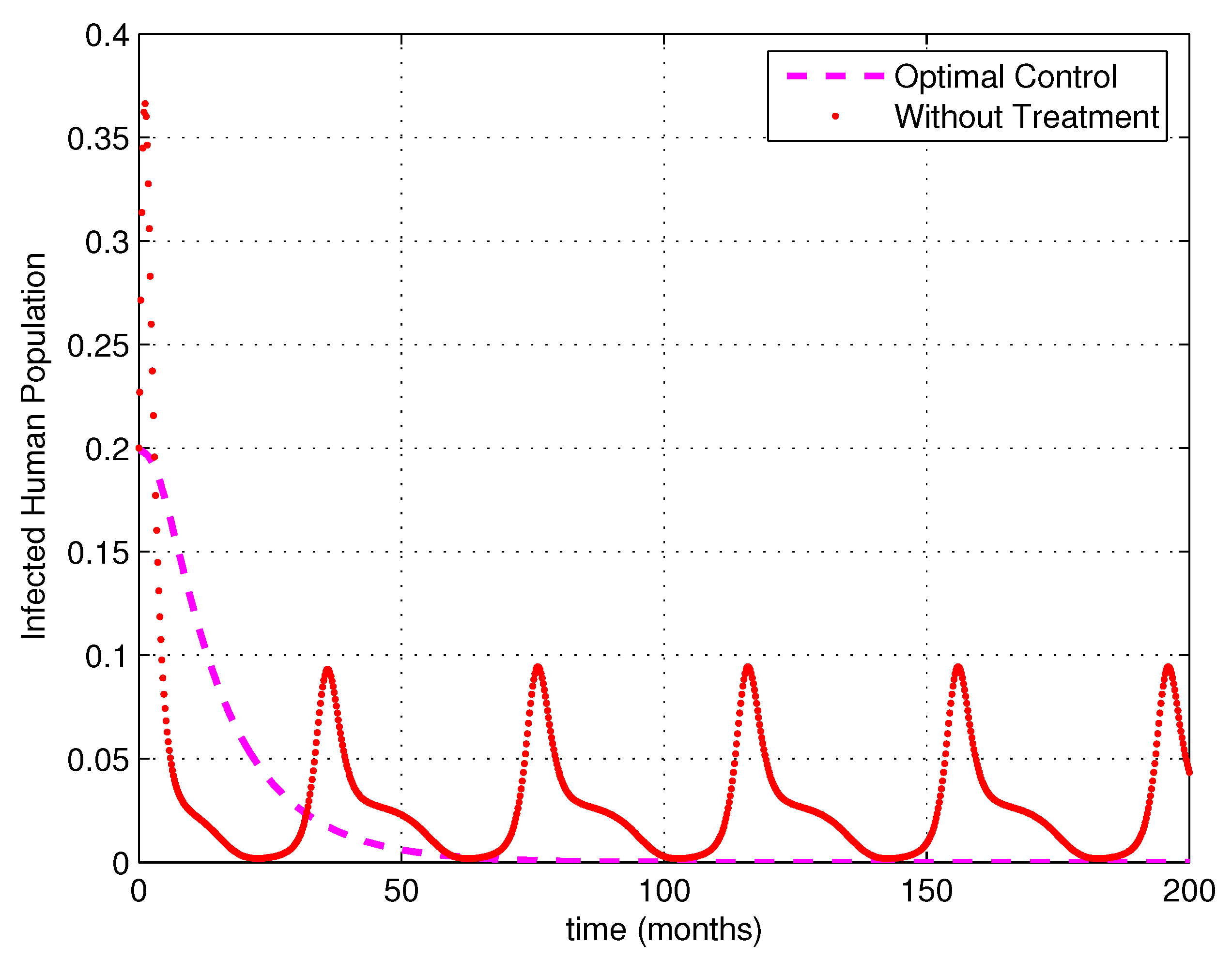
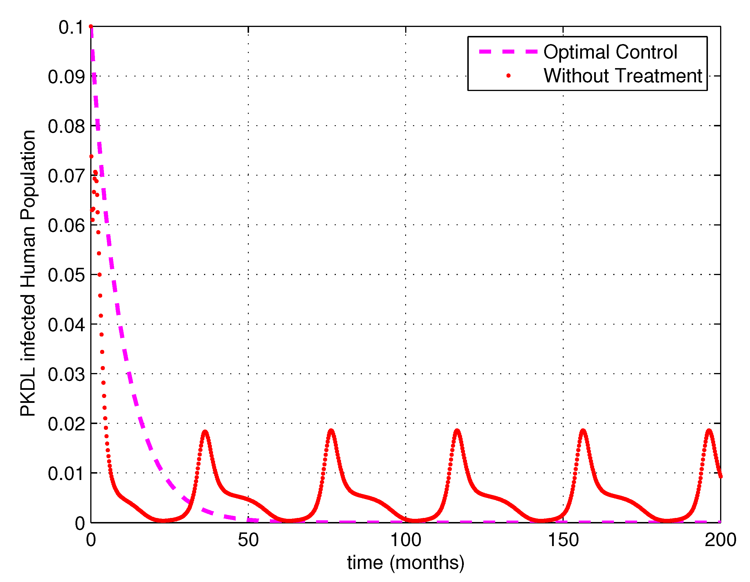
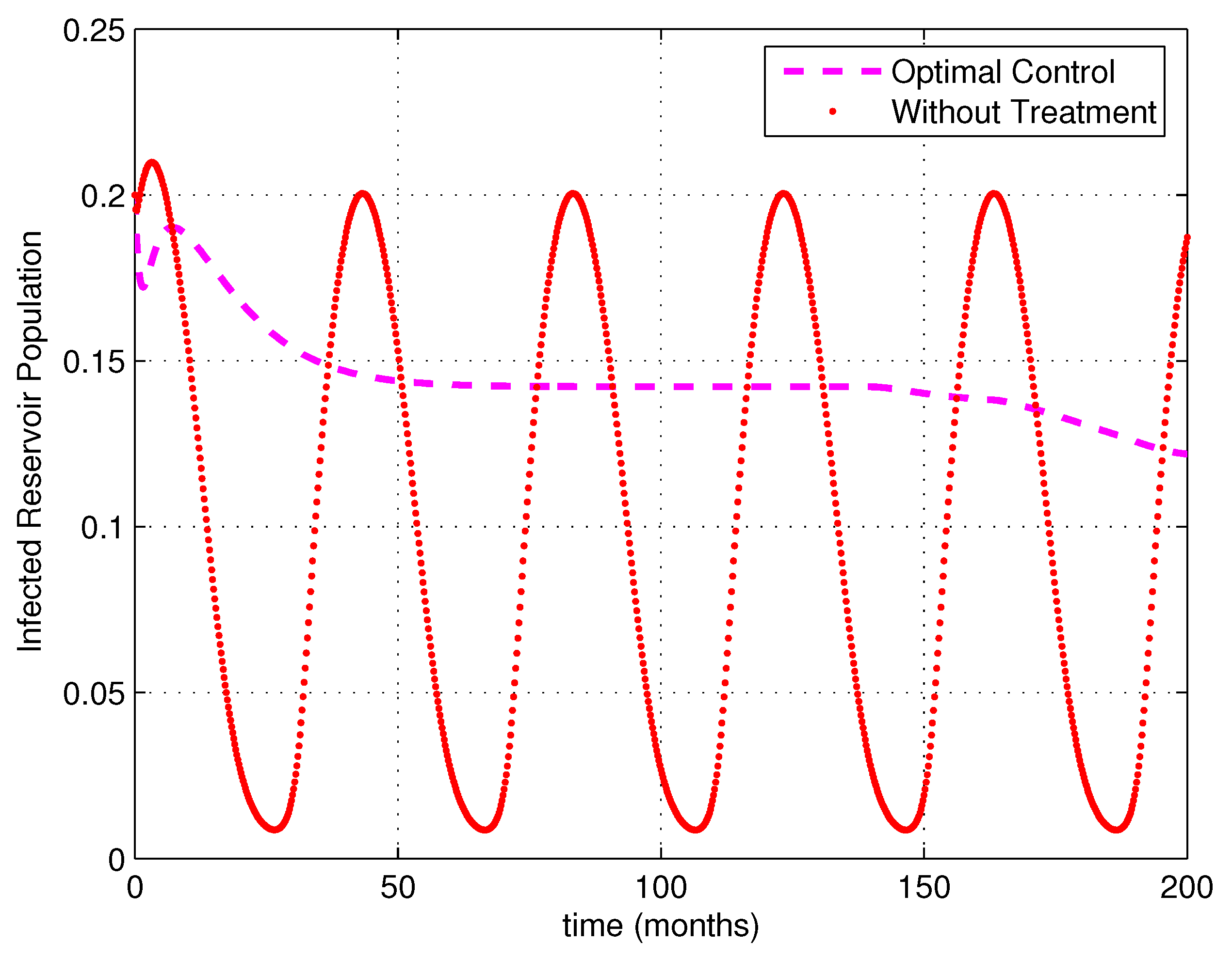
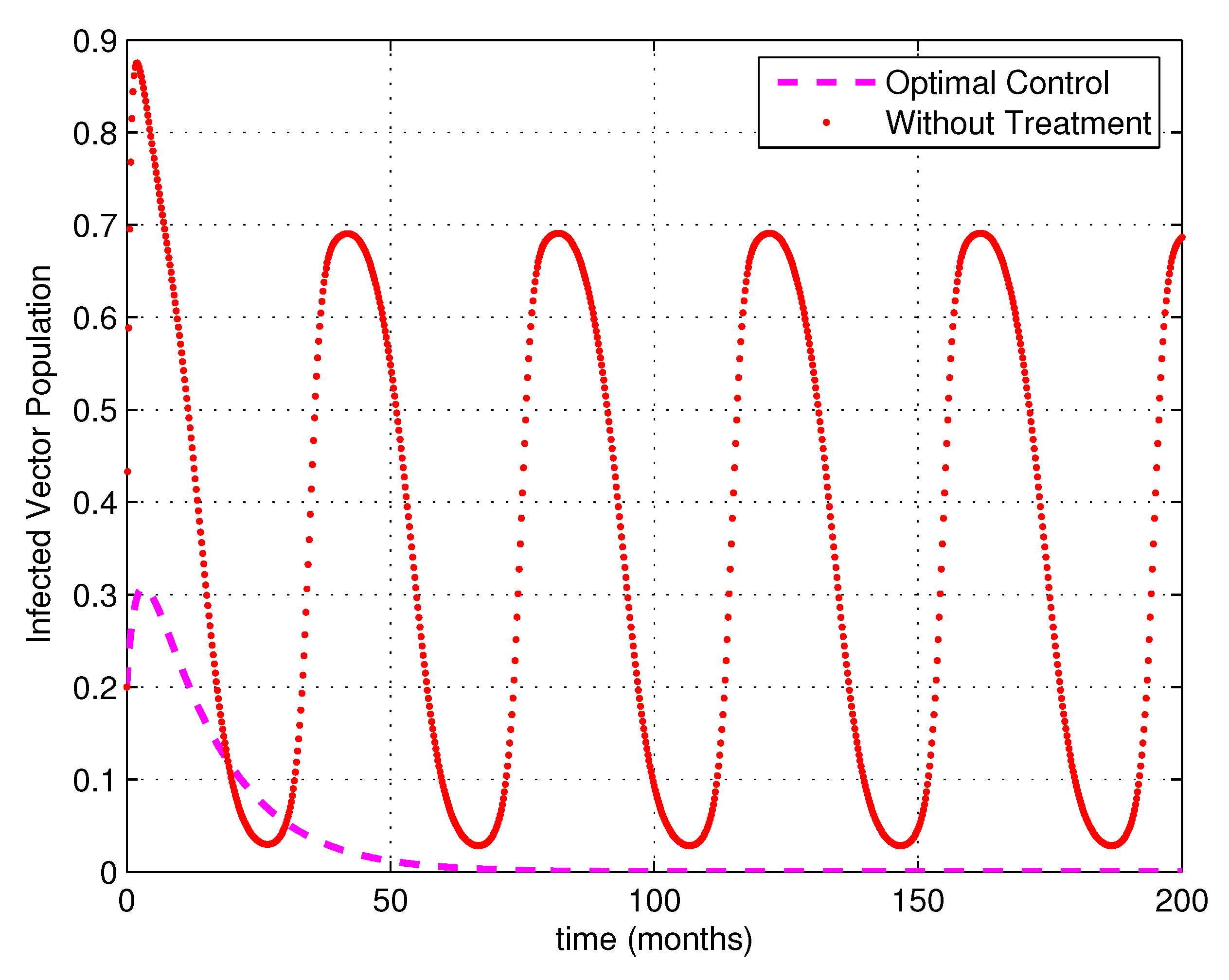
5. Numerical Simulations

In this section, we present some numerical results obtained using data from [18], assuming that the force of infection is a periodic function with a period of 12 months, with one peak in each period. The parameter values are given in Table 1. To solve the optimal control problem, we used a forward-backward Runge–Kutta of order 4 (RK4) method. To solve the state system of ordinary differential equations, a simple forward RK4 method was applied, but to solve the adjoint ODE, the RK4 method had to be adapted to account for solving backwards in time.

In Figure 1, it is clear that without control, the fraction of infected humans decreases to low levels, then starts to increase and repeats this process periodically; however with optimal control, it decreases to a very low level and settles at that level.

Figure 2 shows that the fraction of infected reservoirs without control increases at first, then decreases to a very low level, before increasing again; this process is repeated, and the fraction of infected reservoirs with control increases at first, then decreases again and settles on a medium level. This is because there is no control applied to the reservoir population.

From Figure 3, it is clear that the fraction of infected vectors without control increases at first, then decreases to a low level, before increasing again; this process is repeated, and the fraction of infected vectors with control increases slightly at first, then decreases again and settles on a very low level. The reason is that the control applied to the human population affects the vector population indirectly.

In Figure 4, we show that without control, the fraction of PKDL-infected humans decreases at first, then increases; this process repeats again until the end of the simulation time, while with control, this fraction decreases to a very low level.

The main conclusion drawn from the simulation is that when the optimal control is applied, the periodicity disappears from the model.

6. Discussion

Visceral leishmaniasis is associated with many different factors, such as complex vector dynamics, the role of an animal reservoir, and social and economical factors; one of the most important factors is the seasonal dynamics of the disease, which makes its control very difficult, as seasonality makes the recurrence of epidemics very common.

In this paper, we present and analyze a mathematical model for the dynamics of visceral leishmaniasis, assuming that the biting rate of the vector is a time-dependent function, to capture the seasonal behavior of the disease. Our results show that if ${\mathcal{R}}_0$ is less than unity, then the disease-free equilibrium is globally asymptotically stable, and if ${\mathcal{R}}_0>1$, then our system is uniformly persistent and admits at least one positive $\omega$-periodic solution. Two time-dependent control variables, namely, the treatment of infected humans and the vaccination of susceptible individuals, were added to the model in order to investigate the best control strategy against the disease. The analysis and numerical simulation of the optimal control problem show that using an optimal combination of vaccination and treatment will make the system periodic-free by forcing it to reach the disease-free state. The optimal combination of vaccination and treatment means that an extensive use of treatment for all infected individuals and massive vaccination for susceptible humans should be applied. As shown previously, there is not yet a vaccine for visceral leishamaniasis; however, our results suggest that the research should continue to develop such as vaccine, as if it is applied perfectly with the treatment, it will lead to a disease-free state of the system, and more importantly, it will stop the recurrence of the disease. Our model assumes that vaccinated individuals could not be infected with visceral leishmaniasis and that the waning rate of the vaccine is very low; therefore the developed vaccine should be very effective to achieve these goals. Our results also suggest that the vaccine should be very cheap or otherwise freely distributed, as it should be applied widely, and almost all of the susceptible individuals should be vaccinated to eradicate the disease.

References

1. Chaves, L.F.; Pascual, M. Climate Cycles and Forecasts of Cutaneous Leishmaniasis, a Nonstationary Vector-Borne Disease. PLoS Med. 2006, 3, 1320–1328. [Google Scholar] [CrossRef] [PubMed]
2. Reithinger, R.; Jean-Claude, D.; Hechmi, L.; Claude, P.; Bruce, A.; Simon, B. Cutaneous leishmaniasis. Lancet Infect. Dis. 2007, 7, 581–596. [Google Scholar] [CrossRef]
3. Zijlstra, E.E.; Musa, A.M.; Khalil, E.A.; el-Hassan, I.M.; el-Hassan, A.M. Post-kala-azar dermal leishmaniasis. Lancet Infect. Dis. 2003, 3, 87–98. [Google Scholar] [CrossRef]
4. Schriefer, A.; Luiz, H.G.; Paulo, R.L.M.; Marcus, L.; Hélio, A.L.; Ednaldo, L.; Guilherme, R.; Aristóteles, G.-N.; Ana, L.F.S.; Lee, W.R.; et al. Geographic Clustering of Leishmaniasis in Northeastern Brazil. Emerg. Infect. Dis. 2009, 15, 871–876. [Google Scholar] [CrossRef] [PubMed]
5. Ibrahim, A.A.; Abdoon, M.A.A. Distribution and population dynamics of phlebotomus Sandflies in an endemic area of cutaneous leishmaniasis in Asir Region. J. Entomol. 2005, 2, 102–108. [Google Scholar]
6. Al-Tawfiq, J.A.; Abu-Khams, A. Cutaneous leishmaniasis: A 46-year study of the epidemiology and clinical features in Saudi Arabia (1956–2002). Int. J. Infect. Dis. 2004, 8, 244–250. [Google Scholar] [CrossRef] [PubMed]
7. Cardenas, R.; Claudia, M.; Alfonso, J.; Franco-Paredes, C. Studied impact of climate change variability in the occurrence of leishmaniasis in Northeastern Colombia. Am. J. Trop. Med. Hyg. 2006, 75, 273–277. [Google Scholar] [PubMed]
8. Cross, E.R.; Newcomb, W.W.; Tucker, C.J. Use of weather data and remote sensing to predict the geographic and seasonal distribution of phlebotomus papatasi in Southwest Asia. Am. J. Trop. Med. Hyg. 1996, 56, 530–536. [Google Scholar] [CrossRef]
9. Tiwary, P.; Kumar, D.; Mishra, M.; Singh, R.P.; Rai, M.; Sundar, S. Seasonal Variation in the Prevalence of Sand Flies Infected with Leishmania donovani. PLoS ONE 2013, 8, e61370. [Google Scholar] [CrossRef] [PubMed]
10. Turki, K.F.; Iain, R.L. The Seasonality of Cutaneous Leishmaniasis in Asir Region, Saudi Arabia. Int. J. Environ. Sustain. 2014, 3, 1–13. [Google Scholar]
11. Beaumier, C.M.; Gillespie, P.M.; Hotez, P.J.; Bottazzi, M.E. New vaccines for neglected parasitic diseases and dengue. Transl. Res.: J. Lab. Clin. Med. 2013, 162, 144–155. [Google Scholar] [CrossRef] [PubMed]
12. Dye, C. The Logic of Visceral Leishmaniasis control. Am. J. Trop. Med. Hyg. 1996, 55, 125–130. [Google Scholar] [CrossRef] [PubMed]
13. Dye, C.; Williams, B.G. Malnutrition, age and risk of parasitic disease: Visceral leishmaniasis revisited. Proc. R. Soc. Lond. Ser. B 1993, 254, 33–39. [Google Scholar] [CrossRef] [PubMed]
14. Lysenko, A.J.; Beljaev, A.E. Quantitative Approaches to Epidemiology; Peters, W., Killick-Kendrick, R., Eds.; The Leishmaniasis in Biology and Medicine; Academic Press: London, UK, 1987; pp. 263–290. [Google Scholar]
15. Rabinovich, J.E.; Feliciangeli, M.D. Arameters of leishmania braziliensis transmission by indoor Lutzomyia ovallesi in Venezuela. Am. J. Trop. Med. Hyg. 2004, 70, 373–382. [Google Scholar] [PubMed]
16. Burattini, M.N.; Coutinho, F.A.B.; Lopez, L.F.; Massad, E. Modeling the dynamics of leishmaniasis considering human, animal host and vector populations. J. Biol. Syst. 1998, 6, 337–356. [Google Scholar] [CrossRef]
17. Osman, O.F.; Kager, P.A.; Oskam, L. Lieshmaniasis in the Sudan: A literature review with emphasis on clinical aspects. Trop. Med. Int. Health 2000, 5, 553–562. [Google Scholar] [CrossRef] [PubMed]
18. Elmojtaba, I.M.; Mugisha, J.Y.T.; Hashim, M.H.A. Mathematical analysis of the dynamics of visceral leishmaniasis in the Sudan. Appl. Math. Comput. 2010, 217, 2567–2578. [Google Scholar] [CrossRef]
19. Elmojtaba, I.M.; Mugisha, J.Y.T.; Hashim, M.H.A. Modeling the role of cross immunity between two different strains of leishmania. Nonlinear Anal.: Real World Appl. 2010, 11, 2175–2189. [Google Scholar] [CrossRef]
20. Elmojtaba, I.M. Mathematical model for the dynamics of visceral leishmaniasis–malaria co-infection. Math. Methods Appl. Sci. 2016, 39, 4334–4353. [Google Scholar] [CrossRef]
21. Elmojtaba, I.M.; Mugisha, J.Y.T.; Hashim, M.H.A. Vaccination Model for Visceral Leishmaniasis with infective immigrants. Math. Methods Appl. Sci. 2013, 36, 216–226. [Google Scholar] [CrossRef]
22. Zhang, F.; Zhao, X.-Q. A periodic epidemic model in patchy environment. J. Math. Anal. Appl. 2007, 325, 496–516. [Google Scholar] [CrossRef]
23. Wang, W.; Zhao, X.-Q. Threshold Dynamics for compartmental Epidemic Models in Periodic Environments. J. Dyn. Diff. Equ. 2008, 20, 699–717. [Google Scholar] [CrossRef]
24. Smith, H.L.; Waltman, P. The Theory of the Chemostat: Dynamics of Microbial Competition; Cambridge University Press: London, UK, 1995. [Google Scholar]
25. Thieme, H.R. Convergence results and Poincare-Bendixson trichotomy for asymptomatically autonomous differential equations. J. Math. Biol. 1992, 30, 755–763. [Google Scholar] [CrossRef]
26. Zhao, X.-Q. Dynamical Systems in Population Biology; Springer: New York, NY, USA, 2003. [Google Scholar]
27. Hale, J.K. Asymptotic Behavior of Dissipative Systems; American Mathematical Society: Providence, RI, USA, 1988. [Google Scholar]
28. Zhu, Y.; Wang, K. Existence and global attractivity of positive periodic solutions for a predator-prey model with modified Laslie-Gower Holling-type II schemes. J. Math. Anal. Appl. 2011, 384, 400–408. [Google Scholar] [CrossRef]
29. Gemperli, A.; Vounatsou, P.; Sogoba, N.; Smith, T. Malaria mapping using transmission models: Application to survey data from Mali. Am. J. Epidemiol. 2006, 163, 289–297. [Google Scholar] [CrossRef] [PubMed]
30. Kasap, O.E.; Alten, B. Comparative demography of the sand fly Phlebotomus papatasi (Diptera: Psychodidae) at constant temperatures. J. Vect. Ecol. 2006, 31, 378–385. [Google Scholar] [CrossRef]
31. Coutinho, F.A.B.; Burattini, M.N.; Lopez, L.F.; Massad, E. An approximate threshold condition for non-autonomous system: An application to a vector-borne infection. Math. Comput. Simul. 2005, 70, 149–158. [Google Scholar] [CrossRef]
32. Lainson, R.; Ryan, L.; Shaw, J.J. Infective stages of Leishmania in the sandfly vector and some observations on the mechanism of transmission. Memórias Inst. Oswaldo Cruz 1987, 82, 421–424. [Google Scholar] [CrossRef]
33. Gasim, S.; Elhassan, A.M.; Kharazmi, A.; Khalil, E.A.G.; Ismail, A.; Theander, T.G. The development of post-kala-azar dermal leishmaniasis (PKDL) is associated with acquisition of Leishmania reactivity by peripheral blood mononuclear cells (PBMC). Clin. Exp. Immunol. 2000, 119, 523–529. [Google Scholar] [CrossRef] [PubMed]
34. Sundar, S.; Lockwood, D.N.J.; Agrawal, G.; Rai, M.; Makharia, M.K.; Murray, H.W. Treatment of Indian visceral leishmaniasis with single or daily infusions of low dose liposomal amphotericin B: Randomised trial Commentary: Cost and resistance remain issues. BMJ 2001, 323, 419–422. [Google Scholar] [CrossRef] [PubMed]
35. Pontryagin, L.S. Mathematical Theory of Optimal Processes; CRC Press: Boca Raton, FL, USA, 1987. [Google Scholar]
36. Yusuf, T.T.; Benyah, F. Optimal control of vaccination and treatment for an SIR epidemiological model. World J. Model. Simul. 2008, 8, 194–204. [Google Scholar]
37. Lenhart, S.; Workman, J.T. Optimal Control Applied to Biological Models; CRC Press: Boca Raton, FL, USA, 2007. [Google Scholar]
38. Fleming, W.H.; Rishel, R.W. Deterministic and Stochastic Optimal Control; Springer: New York, NY, USA, 2012. [Google Scholar]
Figure 1. Simulation results showing the infected humans.
Mathematics 05 00080 g001
Figure 2. Simulation results showing the infected reservoir.
Mathematics 05 00080 g002
Figure 3. Simulation results showing the infected vector.
Mathematics 05 00080 g003
Figure 4. Simulation results showing post-kala-azar dermal leishmaniasis (PKDL).
Mathematics 05 00080 g004