A Two-Stage Method for Piecewise-Constant Solution for Fredholm Integral Equations of the First Kind

Abstract

A numerical method is proposed for estimating piecewise-constant solutions for Fredholm integral equations of the first kind. Two functionals, namely the weighted total variation (WTV) functional and the simplified Modica-Mortola (MM) functional, are introduced. The solution procedure consists of two stages. In the first stage, the WTV functional is minimized to obtain an approximate solution ${\mathbf{f}}_{\mathrm{TV}}^{*}$. In the second stage, the simplified MM functional is minimized to obtain the final result by using the damped Newton (DN) method with ${\mathbf{f}}_{\mathrm{TV}}^{*}$ as the initial guess. The numerical implementation is given in detail, and numerical results of two examples are presented to illustrate the efficiency of the proposed approach.

1. Introduction

In many physical problems, the relation between the quantity observed and the quantity to be measured can be formulated as a Fredholm integral equation of the first kind:

$${\int }_0^{1}k(x,t)f\left(t\right)dt=g\left(x\right),0\le x\le 1,$$

(1)

where the kernel function k and the right-hand side g are known, while f is the unknown to be determined. The Fredholm integral equation of the first kind is ill-posed; see for instance [1], Chapter 2.

In practical applications, there is noise in the right-hand side; therefore, Equation (1) should be revised as:

$${\int }_0^{1}k(x,t)f\left(t\right)dt=g\left(x\right)+\eta \left(x\right),0\le x\le 1,$$

where $\eta$ represents the error. The above equation can be written in the operator form:

$$\mathcal{K}f=h,$$

(2)

where $\left(\mathcal{K}f\right)\left(x\right)={\int }_0^{1}k(x,t)f\left(t\right)dt$, $0\le x\le 1$ and $h=g+\eta$.

Numerical methods for obtaining a reasonable approximate solution to the Fredholm integral equation of the first kind have attracted many researchers, and many research results have been achieved; see, for instance, ([2], Chapter 12), and [3,4,5,6,7]. Due to the ill-posedness nature of the problem, numerical solutions are extremely sensitive to perturbations caused by observation and rounding errors. Therefore, regularization is required to obtain a reasonable approximate solution. Many regularization methods have been proposed; see, for instance, [8] Chapters 2 and 8. The Tikhonov regularization method [9], the truncated singular value decomposition (TSVD) method [10], the modified TSVD (MTSVD) method [11], the Chebyshev interpolation method [12], the collocation method [13,14], the projected Tikhonov regularization method [15], and so on, are applied to obtain approximate continuous solutions of Equation (2). The total variation (TV) regularization method [16,17,18,19,20,21,22], adaptive TV methods [23,24,25,26,27], the piecewise-polynomial TSVD (PP-TSVD) method [28], and so on, are applied to obtain approximate piecewise-continuous solutions.

In this paper, we focus on the case where the solution of Equation (1) is piecewise-constant and the possible function values are known, that is:

$$\prod _{p=1}^m(f\left(x\right)-c_p)=0,x\in [0,1],$$

where $c_1<c_2<\cdots <c_m$ are given constants. This kind of problem arises in many applications, for instance barcode reading, where $m=2$, $c_1=0$, $c_2=1$, and image restoration, where $m=256$, $c_p=p-1$, $p=1,2,\dots ,256$.

This paper is organized as follows. In Section 2, two objective functionals are introduced; one is based on a weighted TV functional to allow the TV regularization to be spatially varying, and the other one is based on a simplified Modica-Mortola (MM) functional to make use of the a priori knowledge of the solution. In Section 3, the implementation of numerical methods for solving Equation (2) is presented in detail. In Section 4, numerical examples are presented to illustrate the effectiveness of the proposed approach. Finally, concluding remarks are given in Section 5.

2. The Objective Functionals

The TV regularization method has been shown to be an effective way to estimate piecewise-constant solutions. This method looks for a numerical solution that has small TV, which is not inclined to a continuous or discontinuous solution. The weighted TV regularization scheme is more efficient [23], which allows the TV regularization to be spatially varying, that is a small weight is used if there is a possible edge and a large weight if there is no edge.

A commonly-used weighted TV functional is defined by:

$${\mathrm{TV}}_{\omega ,\beta }\left(f\right)={\int }_0^1\omega \left(x\right)\sqrt{{\left(f^{\prime }\left(x\right)\right)}^2+\beta }dx,$$

(3)

where $\beta >0$ is a parameter and $\omega \left(x\right)\ge 0$ is a weighting function. An example of $\omega \left(x\right)$ is:

$$\omega \left(x\right)=\frac{\theta }{\left|f^{\prime }\left(x\right)\right|+\theta },$$

where $\theta >0$ is a parameter; see [23]. We can see that $0<\omega \left(x\right)\le 1$, and $\omega \left(x\right)$ decreases as $\left|f^{\prime }\left(x\right)\right|$ increases. That is, if $\left|f^{\prime }\left(x\right)\right|$ is large, the corresponding weight is small. The above weighting function is unsmooth, so we modify it as:

$$\omega \left(x\right)=\frac{\sqrt{\beta }+\theta }{\sqrt{{\left(f^{\prime }\left(x\right)\right)}^2+\beta }+\theta }$$

(4)

so that $\omega \left(x\right)$ is smooth and $0<\omega \left(x\right)\le 1$.

One can use the weighted TV functional for Equation (2) to obtain a piecewise-constant solution. In this paper, we consider solving the following minimization problem:

$$\underset{f}{min}{\mathsf{\Phi }}_{\mathrm{TV}}\left(f\right)=\frac{1}{2}J\left(f\right)+\alpha {\mathrm{TV}}_{\omega ,\beta }\left(f\right),$$

(5)

where:

$$J\left(f\right)={\int }_0^1{|\mathcal{K}f-h|}^{2}dx$$

and $\alpha >0$ is a small regularization parameter.

To impose the constraint ${\prod }_{p=1}^m(f\left(x\right)-c_p)=0$ to the numerical solutions, we consider the following simplified MM functional:

$${\mathsf{\Phi }}_{\mathrm{M}}\left(f\right)=\frac{1}{2}J\left(f\right)+\frac{\gamma }{2}\mathrm{M}\left(f\right),$$

(6)

where $\gamma >0$ is a regularization parameter and:

$$\mathrm{M}\left(f\right)={\int }_0^1\prod _{p=1}^m{(f\left(x\right)-c_p)}^{2}dx.$$

Note that the MM functional, which is given by:

$$\frac{1}{2}J\left(f\right)+\frac{\alpha }{2}{\int }_0^1{\left(f^{\prime }\left(x\right)\right)}^{2}dx+\frac{\gamma }{2}\mathrm{M}\left(f\right),$$

(see for instance [29]) is a useful tool for solving constant constraint problems, e.g., Bogosel and Oudet applied the functional to analyze a spectral problem with the perimeter constraint [30].

It must be pointed out that the MM functional $\mathrm{M}\left(f\right)$ is not convex and has many minimal points. In general, we can only obtain a local minimizer for ${\mathsf{\Phi }}_{\mathrm{M}}\left(f\right)$. In other words, the numerical solution obtained by minimizing ${\mathsf{\Phi }}_{\mathrm{M}}\left(f\right)$ depends on the initial guess. This observation motivates us to consider estimating piecewise-constant solutions for (2) by a two-stage method: compute the minimizer $f_{\mathrm{TV}}^{*}$ of ${\mathsf{\Phi }}_{\mathrm{TV}}\left(f\right)$ and then use $f_{\mathrm{TV}}^{*}$ as the initial guess to obtain a minimizer of ${\mathsf{\Phi }}_{\mathrm{M}}\left(f\right)$ to obtain the final result.

2.1. Discretization

To solve the minimization problems (5) and (6) numerically, we need to discretize the relevant functionals. We use the midpoint quadrature and the central divided difference to discretize integrals and first order derivatives, respectively. Let the interval $\left[0,1\right]$ be partitioned uniformly into n subintervals $\left[(i-1)\Delta x,i\Delta x\right]$, $i=1,2,\dots ,n$, then the quadrature points are $\left(i-\frac{1}{2}\right)\Delta x,i=1,2\dots ,n$, where $\Delta x=\frac{1}{n}$. Let $\mathbf{f}={\left[f\left((i-\frac{1}{2})\Delta x\right)\right]}_{i=1}^n$, $\mathbf{h}={\left[h\left((i-\frac{1}{2})\Delta x\right)\right]}_{i=1}^n$ and $K=\Delta x{\left[k\left(\left(i-\frac{1}{2}\right)\Delta x,\left(j-\frac{1}{2}\right)\Delta x\right)\right]}_{i,j=1}^n$. Then, the discretization form of (2) is given by:

$$K\mathbf{f}=\mathbf{h}.$$

The discretization of the functionals $J\left(f\right)$, ${\mathrm{TV}}_{\omega ,\beta }\left(f\right)$, and $\mathrm{M}\left(f\right)$ are as follows.

(1)

The discretization of $J\left(f\right)$ is given by:

$$J\left(\mathbf{f}\right)={\parallel K\mathbf{f}-\mathbf{h}\parallel }^2,$$

where $\parallel ·\parallel$ denotes the vector two-norm.

(2)

Let ${\mathbf{e}}_i$ be the i-th column of the $n\times n$ identity matrix, and let:

$$\begin{array}{c}\hfill {\mathbf{d}}_i={\mathbf{e}}_{i+1}-{\mathbf{e}}_i,i=1,2,\dots ,n-1,\end{array}$$

and:

$$\begin{array}{c}\hfill D=[{\mathbf{d}}_1,{\mathbf{d}}_2,\cdots ,{\mathbf{d}}_{n-1}].\end{array}$$

We approximate the weighted TV functional ${\mathrm{TV}}_{\omega ,\beta }\left(f\right)$ (cf. (3)) by:

$${\mathrm{TV}}_{\omega ,\beta }\left(\mathbf{f}\right)=\sum _{i=1}^{n-1}{\omega }_i\psi \left({\mathbf{d}}_i^T\mathbf{f}\right),$$

where ${\omega }_i=\omega ((i-1/2)\Delta x)$ and $\psi \left(x\right)=\sqrt{x^2+\beta }$ (we replace $\beta {(\Delta x)}^2$ by $\beta$ for the sake of simplicity). Obviously, if the weighting factors are set to ${\omega }_i=1$, $i=1,2,\dots ,n-1$, the weighted TV functional is just the traditional TV functional. In this paper, we choose smooth factors by approximating (4):

$${\omega }_i=\frac{\sqrt{\beta }+\theta }{\sqrt{{\left({\mathbf{d}}_i^T\mathbf{f}\right)}^2+\beta }+\theta },i=1,2,\dots ,n-1.$$

(7)

(3)

As for $\mathrm{M}\left(f\right)$, we simply approximate it by:

$$\mathrm{M}\left(\mathbf{f}\right)=\sum _{i=1}^n\prod _{p=1}^m{(f_i-c_p)}^2.$$

Here, we omit the factor $\Delta x$ for the sake of simplicity.

Therefore, the discretization of ${\mathsf{\Phi }}_{\mathrm{TV}}\left(f\right)$ is:

$${\mathsf{\Phi }}_{\mathrm{TV}}\left(\mathbf{f}\right)=\frac{1}{2}{\parallel K\mathbf{f}-\mathbf{h}\parallel }^2+\alpha \sum _{i=1}^{n-1}{\omega }_i\psi \left({\mathbf{d}}_i^T\mathbf{f}\right)$$

(8)

and the discretization of ${\mathsf{\Phi }}_{\mathrm{M}}\left(f\right)$ is:

$${\mathsf{\Phi }}_{\mathrm{M}}\left(\mathbf{f}\right)=\frac{1}{2}{\parallel K\mathbf{f}-\mathbf{h}\parallel }^2+\frac{\gamma }{2}\sum _{i=1}^n\prod _{p=1}^m{(f_i-c_p)}^2.$$

(9)

3. Numerical Implementation

In this section, the implementation of the damped Newton (DN) method for minimization of the functions ${\mathsf{\Phi }}_{\mathrm{TV}}\left(\mathbf{f}\right)$ and ${\mathsf{\Phi }}_{\mathrm{M}}\left(\mathbf{f}\right)$ (cf. (8) and (9)) is given. We first derive the gradients and the Hessians of $J\left(\mathbf{f}\right)$, ${\mathrm{TV}}_{\omega ,\beta }\left(\mathbf{f}\right)$ and $\mathrm{M}\left(\mathbf{f}\right)$.

Lemma 1.

Let β and θ be positive constants, and define:

$$\varphi \left(x\right)=\frac{1}{\sqrt{x^2+\beta }},\rho \left(x\right)=\frac{1}{\sqrt{x^2+\beta }+\theta }.$$

(10)

(1) The gradient and the Hessian of $J\left(\mathbf{f}\right)={\parallel K\mathbf{f}-\mathbf{h}\parallel }^2$ are given by:

$$\mathrm{grad}J\left(\mathbf{f}\right)=2K^T(K\mathbf{f}-\mathbf{h})$$

(11)

and:

$$\mathrm{Hess}J\left(\mathbf{f}\right)=2K^{T}K,$$

(12)

respectively.

(2) Let ${\omega }_i=1$, $i=1,2,\dots ,n-1$ and $\varphi \left(x\right)$ be defined by (10). Let $\mathrm{diag}(\varphi \left({\mathbf{d}}_1^T\mathbf{f}\right),\dots ,\varphi \left({\mathbf{d}}_{n-1}^T\mathbf{f}\right))$ be denoted by $\mathrm{diag}\left(\varphi \left(D^T\mathbf{f}\right)\right)$. Then, the gradient and the Hessian of ${\mathrm{TV}}_{\omega ,\beta }\left(\mathbf{f}\right)$ are given by:

$$\mathrm{grad}{\mathrm{TV}}_{\omega ,\beta }\left(\mathbf{f}\right)=L\left(\mathbf{f}\right)\mathbf{f}$$

(13)

and:

$$\mathrm{Hess}{\mathrm{TV}}_{\omega ,\beta }\left(\mathbf{f}\right)=L\left(\mathbf{f}\right)+L^{\prime }\left(\mathbf{f}\right)\mathbf{f},$$

(14)

respectively, where:

$$L\left(\mathbf{f}\right)=D\left[\mathrm{diag}\left(\varphi \left(D^T\mathbf{f}\right)\right)\right]D^T$$

(15)

and:

$$L^{\prime }\left(\mathbf{f}\right)\mathbf{f}=-D\left[{\left(\mathrm{diag}\left(D^T\mathbf{f}\right)\right)}^2{\left(\mathrm{diag}\left(\varphi \left(D^T\mathbf{f}\right)\right)\right)}^3\right]D^T.$$

Here, we use the symbols $L\left(\mathbf{f}\right)$ and $L^{\prime }\left(\mathbf{f}\right)\mathbf{f}$ in the same way as they have been used in [8].

(3) Let ${\omega }_i$, $i=1,2,\dots ,n-1$, be given by (7), and $\varphi \left(x\right)$ and $\rho \left(x\right)$ be defined by (10). Let $\mathrm{diag}(\rho \left({\mathbf{d}}_1^T\mathbf{f}\right),\dots ,\rho \left({\mathbf{d}}_{n-1}^T\mathbf{f}\right))$ be denoted by $\mathrm{diag}\left(\rho \left(D^T\mathbf{f}\right)\right)$. Then, the gradient and the Hessian of ${\mathrm{TV}}_{\omega ,\beta }\left(\mathbf{f}\right)$ are given by:

$$\mathrm{grad}{\mathrm{TV}}_{\omega ,\beta }\left(\mathbf{f}\right)=L\left(\mathbf{f}\right)\mathbf{f}$$

(16)

and:

$$\mathrm{Hess}{\mathrm{TV}}_{\omega ,\beta }\left(\mathbf{f}\right)=L\left(\mathbf{f}\right)+L^{\prime }\left(\mathbf{f}\right)\mathbf{f},$$

(17)

respectively, where:

$$L\left(\mathbf{f}\right)=\tilde{\theta }D\left[\mathrm{diag}\left(\varphi \left(D^T\mathbf{f}\right)\right)\mathrm{diag}{\left(\rho \left(D^T\mathbf{f}\right)\right)}^2\right]D^T$$

(18)

and:

$$L^{\prime }\left(\mathbf{f}\right)\mathbf{f}=-\tilde{\theta }D\left[{\left(\mathrm{diag}\left(D^T\mathbf{f}\right)\right)}^2(\mathrm{diag}\left(\varphi \left(D^T\mathbf{f}\right)\right)+2\mathrm{diag}\left(\rho \left(D^T\mathbf{f}\right)\right))\mathrm{diag}{\left(\rho \left(D^T\mathbf{f}\right)\right)}^2\mathrm{diag}{\left(\varphi \left(D^T\mathbf{f}\right)\right)}^2\right]D^T$$

(19)

with $\tilde{\theta }=\theta (\sqrt{\beta }+\theta )$.

(4) The gradient of $\mathrm{M}\left(\mathbf{f}\right)$ is given by:

$$\mathrm{grad}\mathrm{M}\left(\mathbf{f}\right)={\left(\frac{\partial \mathrm{M}}{\partial f_1},\frac{\partial \mathrm{M}}{\partial f_2},\dots ,\frac{\partial \mathrm{M}}{\partial f_n}\right)}^T,$$

(20)

where the partial derivatives $\frac{\partial \mathrm{M}}{\partial f_i}$, $i=1,2,\dots ,n$, are given by:

$$\begin{array}{ccc}\hfill \frac{\partial \mathrm{M}}{\partial f_i}& =& \left\{\begin{array}{cc}{\displaystyle 2{\left(\prod _{p=1}^m(f_i-c_p)\right)}^2\sum _{p=1}^m\frac{1}{f_i-c_p},}& \prod _{p=1}^m(f_i-c_p)\ne 0,\\ 0,& \prod _{p=1}^m(f_i-c_p)=0.\end{array}\right.\hfill \end{array}$$

(21)

The Hessian of $\mathrm{M}\left(\mathbf{f}\right)$ is a diagonal matrix given by:

$$\mathrm{Hess}\mathrm{M}\left(\mathbf{f}\right)=\mathrm{diag}\left(\frac{{\partial }^2\mathrm{M}}{\partial f_1^2},\frac{{\partial }^2\mathrm{M}}{\partial f_2^2},\cdots ,\frac{{\partial }^2\mathrm{M}}{\partial f_n^2}\right),$$

(22)

where:

$$\frac{{\partial }^2\mathrm{M}}{\partial f_i^2}=\left\{\begin{array}{cc}{\displaystyle 2{\left(\prod _{p=1}^m(f_i-c_p)\right)}^2\left[2{\left(\sum _{p=1}^m\frac{1}{f_i-c_p}\right)}^2-\sum _{p=1}^m\frac{1}{{(f_i-c_p)}^2}\right],}& \prod _{p=1}^m(f_i-c_p)\ne 0,\\ {\displaystyle 2\prod _{p=1,p\ne p_0}^m{(f_i-c_p)}^2,}& f_i=c_{p_0}.\end{array}\right.$$

(23)

Proof. 

Results (1) and (2) of the lemma are well known; see [8], Section 8.2.

(3) Let $\zeta \left(x\right)=\frac{\sqrt{x^2+\beta }}{\sqrt{x^2+\beta }+\theta }$, then we have:

$$\begin{array}{ccc}\hfill {\zeta }^{\prime }\left(x\right)& =& \frac{\theta x}{\sqrt{x^2+\beta }{(\sqrt{x^2+\beta }+\theta )}^2}=\theta x\varphi \left(x\right)\rho {\left(x\right)}^2,\hfill \\ \hfill {\zeta }^{″}\left(x\right)& =& \theta \varphi \left(x\right)\rho {\left(x\right)}^2-\theta x^2(\varphi \left(x\right)+2\rho \left(x\right))\rho {\left(x\right)}^2\varphi {\left(x\right)}^2,\hfill \end{array}$$

where $\varphi \left(x\right)$ and $\rho \left(x\right)$ are defined by (10). Let $\tilde{\theta }=\theta (\sqrt{\beta }+\theta )$; it can be easily checked that for any $\mathbf{v}$,

$$\begin{array}{cc}& \frac{d}{d\tau }{\mathrm{TV}}_{\omega ,\beta }{(\mathbf{f}+\tau \mathbf{v})|}_{\tau =0}\hfill \\ =& \sum _{i=1}^{n-1}\tilde{\theta }·\left({\mathbf{d}}_i^T\mathbf{f}\right)·\varphi \left({\mathbf{d}}_i^T\mathbf{f}\right)·\rho {\left({\mathbf{d}}_i^T\mathbf{f}\right)}^2·{\mathbf{d}}_i^T\mathbf{v}\hfill \\ =& \tilde{\theta }·{\left(D^T\mathbf{v}\right)}^T·\mathrm{diag}\left(\varphi \left(D^T\mathbf{f}\right)\right)·\mathrm{diag}{\left(\rho \left(D^T\mathbf{f}\right)\right)}^2·\left(D^T\mathbf{f}\right)\hfill \\ =& ⟨\tilde{\theta }D\left[\mathrm{diag}\left(\varphi \left(D^T\mathbf{f}\right)\right)\mathrm{diag}{\left(\rho \left({\mathbf{d}}_i^T\mathbf{f}\right)\right)}^2\right]D^T\mathbf{f},\mathbf{v}⟩.\hfill \end{array}$$

It follows that:

$$\mathrm{grad}{\mathrm{TV}}_{\omega ,\beta }\left(\mathbf{f}\right)=L\left(\mathbf{f}\right)\mathbf{f},$$

where $L\left(\mathbf{f}\right)$ is given by (18).

To obtain the Hessian of ${\mathrm{TV}}_{\omega ,\beta }$, we consider ${\mathrm{TV}}_{\omega ,\beta }(\mathbf{f}+\tau \mathbf{v}+\xi \mathbf{w})$. From the expression of ${\zeta }^{″}\left(x\right)$, we have that for any $\mathbf{v},\mathbf{w}$:

$$\begin{array}{cc}& \frac{{\partial }^2}{\partial \tau \partial \xi }{\mathrm{TV}}_{\omega ,\beta }{(\mathbf{f}+\tau \mathbf{v}+\xi \mathbf{w})|}_{\tau ,\xi =0}\hfill \\ =& \sum _{i=1}^{n-1}\tilde{\theta }·\varphi \left({\mathbf{d}}_i^T\mathbf{f}\right)·\rho {\left({\mathbf{d}}_i^T\mathbf{f}\right)}^2·{\mathbf{d}}_i^T\mathbf{w}·{\mathbf{d}}_i^T\mathbf{v}\hfill \\ & -\sum _{i=1}^{n-1}\tilde{\theta }·{\left({\mathbf{d}}_i^T\mathbf{f}\right)}^2·(\varphi \left({\mathbf{d}}_i^T\mathbf{f}\right)+2\rho \left({\mathbf{d}}_i^T\mathbf{f}\right))·\rho {\left({\mathbf{d}}_i^T\mathbf{f}\right)}^2·\varphi {\left({\mathbf{d}}_i^T\mathbf{f}\right)}^2·{\mathbf{d}}_i^T\mathbf{w}·{\mathbf{d}}_i^T\mathbf{v}\hfill \\ =& ⟨(L\left(\mathbf{f}\right)+L^{\prime }\left(\mathbf{f}\right)\mathbf{f})\mathbf{w},\mathbf{v}⟩,\hfill \end{array}$$

where $L\left(\mathbf{f}\right)$ and $L^{\prime }\left(\mathbf{f}\right)\mathbf{f}$ are given by (18) and (19) respectively. Consequently:

$$\mathrm{Hess}{\mathrm{TV}}_{\omega ,\beta }\left(\mathbf{f}\right)=L\left(\mathbf{f}\right)+L^{\prime }\left(\mathbf{f}\right)\mathbf{f}.$$

(4) It is easy to see that the partial derivatives $\frac{\partial \mathrm{M}}{\partial f_i}$, $i=1,2,\dots ,n$, are given by:

$$\begin{array}{ccc}\hfill \frac{\partial \mathrm{M}}{\partial f_i}& =& 2\left(\prod _{p=1}^m(f_i-c_p)\right)\left(\sum _{l=1}^m\prod _{p=1,p\ne l}^m(f_i-c_p)\right),\hfill \end{array}$$

which can be rewritten in the form of (21). For the second order partial derivatives, we have:

$$\frac{{\partial }^2\mathrm{M}}{\partial f_i^2}=\left\{\begin{array}{cc}{\displaystyle 2{\left(\prod _{p=1}^m(f_i-c_p)\right)}^2\left[2{\left(\sum _{p=1}^m\frac{1}{f_i-c_p}\right)}^2-\sum _{p=1}^m\frac{1}{{(f_i-c_p)}^2}\right],}& \prod _{p=1}^m(f_i-c_p)\ne 0,\\ {\displaystyle 2\prod _{p=1,p\ne p_0}^m{(f_i-c_p)}^2,}& f_i=c_{p_0},\end{array}\right.$$

and

$$\frac{{\partial }^2\mathrm{M}}{\partial f_i\partial f_j}=0,i\ne j.$$

Therefore, the Hessian of $\mathrm{M}$ is a diagonal matrix given by:

$$\mathrm{Hess}\mathrm{M}\left(\mathbf{f}\right)=\mathrm{diag}\left(\frac{{\partial }^2\mathrm{M}}{\partial f_1^2},\frac{{\partial }^2\mathrm{M}}{\partial f_2^2},\cdots ,\frac{{\partial }^2\mathrm{M}}{\partial f_1^2}\right),$$

where ${\partial }^2\mathrm{M}/\partial f_i^2$, $i=1,2,\dots ,n$, are given by (23). ☐

From Formulas (11)–(23), we can get the gradients and the Hessians of ${\mathsf{\Phi }}_{\mathrm{TV}}\left(\mathbf{f}\right)$ and ${\mathsf{\Phi }}_{\mathrm{M}}\left(\mathbf{f}\right)$. We introduce the following DN method for minimization of $\mathsf{\Psi }\left(\mathbf{f}\right)={\mathsf{\Phi }}_{\mathrm{TV}}\left(\mathbf{f}\right)$ or ${\mathsf{\Phi }}_{\mathrm{M}}\left(\mathbf{f}\right)$.

Algorithm 1: Damped Newton (DN) method for the minimization of $\mathsf{\Psi }\left(\mathbf{f}\right)$.

Input an initial guess ${\mathbf{f}}_0$;   $\nu =0$;   Begin iterations    Compute $\mathbf{g}=\mathrm{grad}\mathsf{\Psi }\left({\mathbf{f}}_{\nu }\right)$ and $H=\mathrm{Hess}\mathsf{\Psi }\left({\mathbf{f}}_{\nu }\right)$;    Solve $H\mathbf{s}=-\mathbf{g}$ to obtain $\mathbf{s}$;    Obtain the minimum point of the one-dimensional nonnegative function $\mathsf{\Psi }({\mathbf{f}}_{\nu }+\tau \mathbf{s})$ by using   line search to get ${\tau }_{\nu }=arg{min}_{\tau }\mathsf{\Psi }({\mathbf{f}}_{\nu }+\tau \mathbf{s})$;    Update the approximate solution: ${\mathbf{f}}_{\nu +1}={\mathbf{f}}_{\nu }+{\tau }_{\nu }\mathbf{s}$;    Check the termination condition: If $\parallel {\mathbf{f}}_{\nu +1}-{\mathbf{f}}_{\nu }\parallel /\parallel {\mathbf{f}}_{\nu +1}\parallel <ϵ$, break;    $\nu =\nu +1$;   End iterations   Output ${\mathbf{f}}_{\nu +1}$.

Remark 1.

(1) Since we carry out exact line search (Step 6) in the iterative process, the DN method converges to a local minimal point if the Hessian of $\mathsf{\Psi }\left(\mathbf{f}\right)$ is invertible. In the case that $\mathsf{\Psi }\left(\mathbf{f}\right)$ is singular, modification is required. In our numerical tests in Section 4, no modification is needed. It must be pointed out that for large-scale systems, the most expensive part of the algorithm is solving $H\mathbf{s}=-\mathbf{g}$ to obtain $\mathbf{s}$. If the matrix H has a Toeplitz structure, then the conjugate gradient method with the fast Fourier transform (FFT) can be applied to solve the system efficiently; see [31] for details.

(2) For the minimization of ${\mathsf{\Phi }}_{\mathrm{TV}}\left(\mathbf{f}\right)$, if we approximate the Hessian of ${\mathsf{\Phi }}_{\mathrm{TV}}\left(\mathbf{f}\right)$ by the positive definite matrix $K^{T}K+\alpha L\left(\mathbf{f}\right)$ (assume that $K\mathbf{1}\ne 0$ where $\mathbf{1}$ is the vector with all elements equal to one) and set the step-size ${\tau }_{\nu }$ to 1, we get the Gauss–Newton method. If we obtain ${\tau }_{\nu }$ by using line search method, we get a modified Gauss–Newton (MGN) method. In this paper, we also consider the MGN method for minimization of ${\mathsf{\Phi }}_{\mathrm{TV}}\left(\mathbf{f}\right)$. Obviously, the MGN method converges to a local minimal point.

To end this section, we state the process for solving Equation (2). We first obtain the minimizer ${\mathbf{f}}_{\mathrm{TV}}^{*}$ of ${\mathsf{\Phi }}_{\mathrm{TV}}\left(\mathbf{f}\right)$, and then, we obtain a minimizer ${\mathbf{f}}_{\mathrm{M}}^{*}$ of ${\mathsf{\Phi }}_{\mathrm{M}}\left(\mathbf{f}\right)$ by using the DN method with ${\mathbf{f}}_{\mathrm{TV}}^{*}$ as the initial guess. The approach can be summarized as Algorithm 2.

Algorithm 2: Weighted total variation Modica-Mortola (WTVMM) method for estimating piecewise-constant solution of Equation (2).

Obtain the minimizer ${\mathbf{f}}_{\mathrm{TV}}^{*}$ of ${\mathsf{\Phi }}_{\mathrm{TV}}\left(\mathbf{f}\right)$ by using the MGN method or the DN method;   Obtain a minimizer ${\mathbf{f}}_{\mathrm{M}}^{*}$ of ${\mathsf{\Phi }}_{\mathrm{M}}\left(\mathbf{f}\right)$ by using the DN method with ${\mathbf{f}}_{\mathrm{TV}}^{*}$ as the initial guess;   Output ${\mathbf{f}}_{\mathrm{M}}^{*}$.

4. Numerical Examples

In this section, we present numerical results for two examples to illustrate that our approach is indeed capable of estimating piecewise-constant solutions to Equation (2).

Besides the numerical solution obtained by using our approach, approximate solutions obtained by using the TV regularization method and the weighted TV regularization method with weighting factors ${\omega }_i=(\sqrt{\beta }+\theta )/(\sqrt{{(f_{i+1}-f_i)}^2+\beta }+\theta )$ (cf. (7)) are presented. In the following tables and figures, we use the symbols weighted total variation Modica-Mortola (WTVMM), TV and WTV to denote the above three methods.

We set the number of subintervals to $n=128$. All tests were carried out by using MATLAB, and the termination parameter is set to $ϵ={10}^{-5}$; see Step 8 of Algorithm 1. In the tables, the column “$(\alpha ,\beta ,\theta ,\gamma )$” gives relevant parameters; the column “$\#it$” gives the number of iterations (for the WTVMM method, $i_1+i_2$ denotes that the WTV method and the MM method require $i_1$ and $i_2$ iterations, respectively). The column “error” gives the relative error defined by:

$$\mathrm{error}=\frac{\parallel {\mathbf{f}}_{\mathrm{exact}}-{\mathbf{f}}_{\mathrm{app}}{\parallel }_2}{\parallel {\mathbf{f}}_{\mathrm{exact}}{\parallel }_2},$$

where ${\mathbf{f}}_{\mathrm{exact}}$ and ${\mathbf{f}}_{\mathrm{app}}$ are the vectors of the exact solution and the approximate solution at the quadrature points, respectively. Here, one iteration refers to Steps 4–8 of Algorithm 1.

There are several regularization parameter choosing methods, e.g., the discrepancy principle, the generalized discrepancy principle, the generalized cross validation, the L-curve and the normalized cumulative periodogram; see, for instance, [32,33], ([1], Chapters 5–6), ([8], Chapter 7), ([34], Chapters 5, 6 and 9). However, we choose the parameters by experiments since there are two additional parameters in the regularization term $T{V}_{\omega ,\beta }\left(\mathbf{f}\right)$. We consider the following rules in choosing the parameters:

(1)

Since we use $\sqrt{x^2+\beta }$ as an approximation of $\left|x\right|$, we set β to a very small positive number. We note that if β is significantly larger than $x^2$, then:

$$\sqrt{x^2+\beta }\approx \sqrt{\beta }+\frac{1}{2\sqrt{\beta }}{x}^2.$$

As a result, the regularization term $\sqrt{x^2+\beta }$ leads to an $H^1$-like regularization.

(2)

If θ is much larger than $x^2$, then the weighting function $\omega \left(x\right)$ is close to one, i.e.,

$$\omega \left(x\right)=\frac{\sqrt{\beta }+\theta }{\sqrt{x^2+\beta }+\theta }\approx 1.$$

It follows that the weighted TV regularization is about the same as the traditional TV regularization. Therefore, we should not choose a large value for θ.

(3)

We choose the value for α by the help of the discrepancy principle and observe if the numerical solution is near piecewise-constant. After choosing a value for α, we consider adjustment of β and θ: if the numerical solution is over-smooth, we choose a smaller value for β or θ; on the other hand, if the numerical solution is oscillating, we choose a larger value for β or θ.

We have tried the DN method and the MGN method for minimization of the functions corresponding to the TV functional (${\omega }_i=1$) and the WTV functional (the weighted factors are given by (7)) in our numerical tests. Numerical results show that the DN method is better than the MGN method when ${\omega }_i=1$, and the MGN method is better than the DN method when ${\omega }_i$ is given by (7). In the following, we show the numerical results carried out by the DN method for minimization of the function corresponding to the TV functional and those carried out by the MGN method for minimization of the function corresponding to the WTV functional.

Example 1.

The kernel of Equation (2) is given by:

$$k(x,t)=\frac{1}{\sigma \sqrt{2\pi }}{e}^{-\frac{{(x-t)}^2}{2{\sigma }^2}},$$

where $\sigma =0.05$. In this case, the condition number of the matrix K is $7.8654\times {10}^{18}$. The right-hand side $g\left(x\right)$ is obtained by setting the exact solution to:

$$f_{\mathrm{exact}}\left(t\right)=\left\{\begin{array}{cc}{c}_1,\hfill & t\in \left[0,0.2\right)\cup \left[0.4,0.6\right)\cup \left[0.8,1\right],\hfill \\ c_2,\hfill & t\in \left[0.6,0.8\right),\hfill \\ c_3,\hfill & t\in \left[0.2,0.4\right),\hfill \end{array}\right.$$

where $c_1=1,c_2=2,c_3=3$. Two noisy right-hand sides, which contain 1% and 10% of white noise, respectively, are tested.

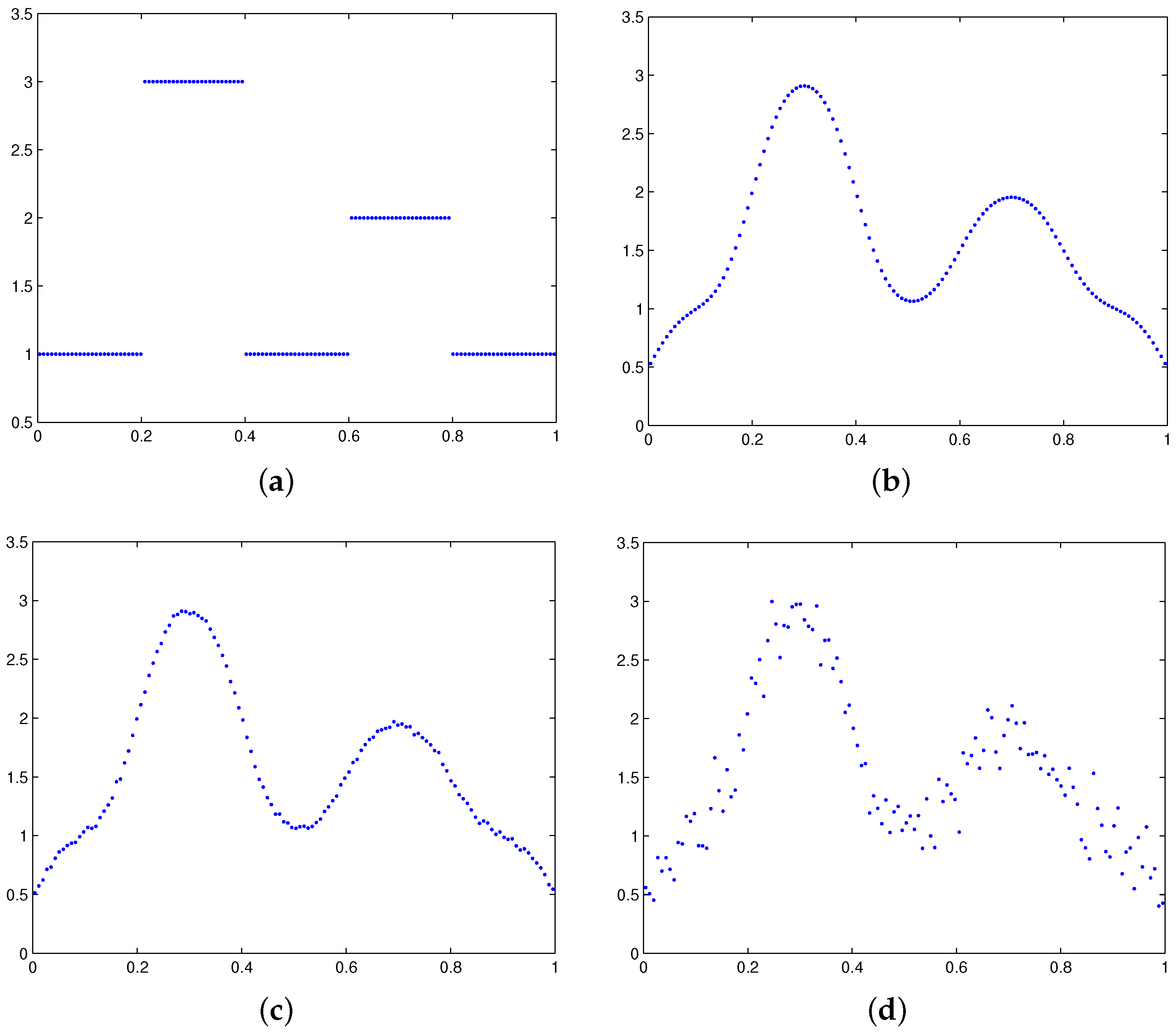
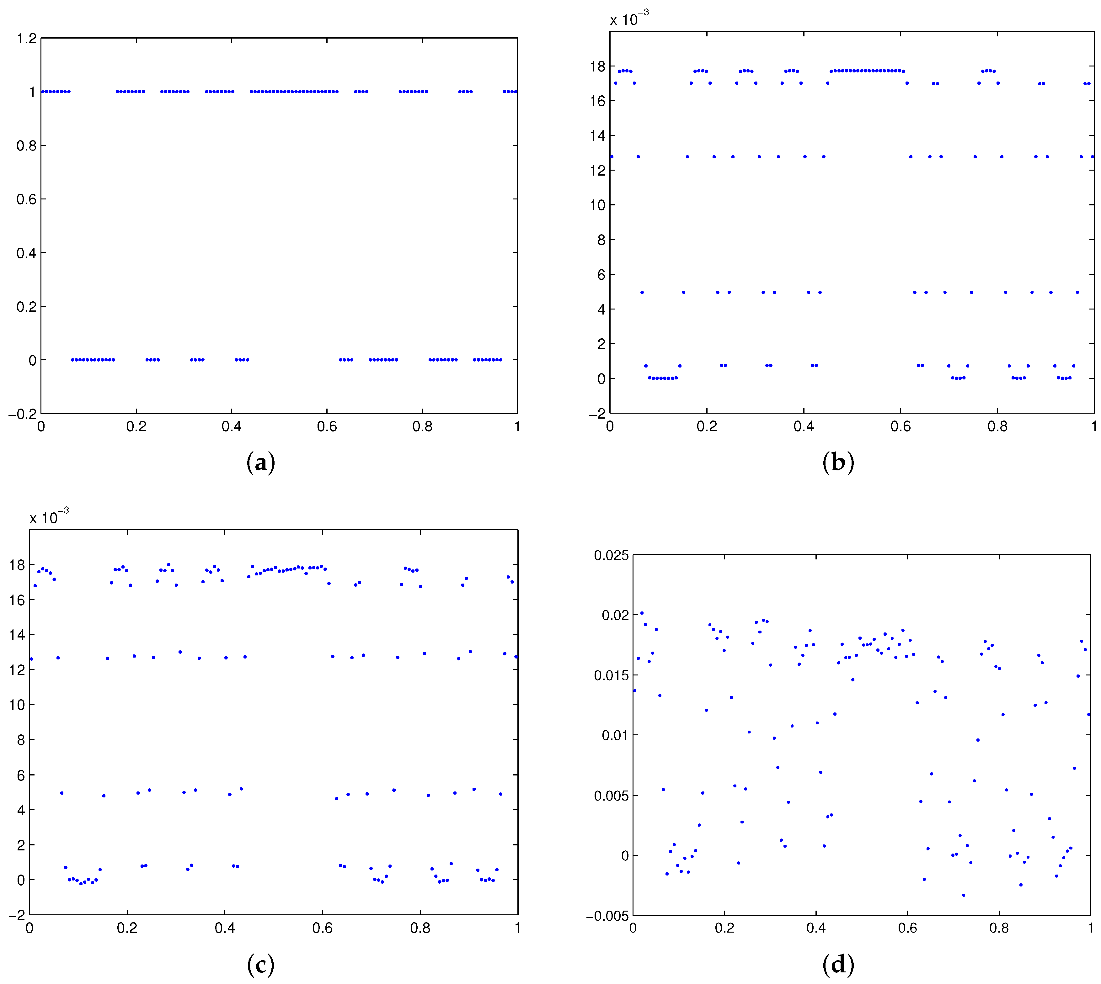
Since the average of $c_1$, $c_2$ and $c_3$ is two, we choose ${\mathbf{f}}_0={(2,2,\dots ,2)}^T$ as the initial guess for the minimization of the functions corresponding to the TV and WTV functionals, which is not too far from the exact solution. The exact solution and the right-hand side are shown in Figure 1a,b, two noisy right-hand sides are shown in Figure 1c,d, respectively. Numerical solutions obtained by different methods, as well as the point-wise error for all numerical solutions are shown in Figure 2. The relevant parameters, the numbers of iterations and the relative errors are given in Table 1 and Table 2.

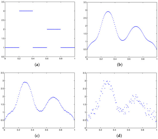
Figure 1. The exact solution, the right-hand side and noisy right-hand sides for Example 1. (a) The exact solution; (b) the right-hand side; (c) a noisy right-hand side containing $1\%$ of white noise; and (d) a noisy right-hand side containing $10\%$ of white noise.

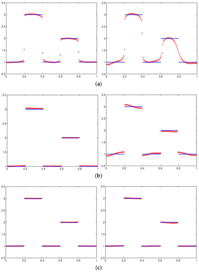
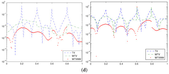
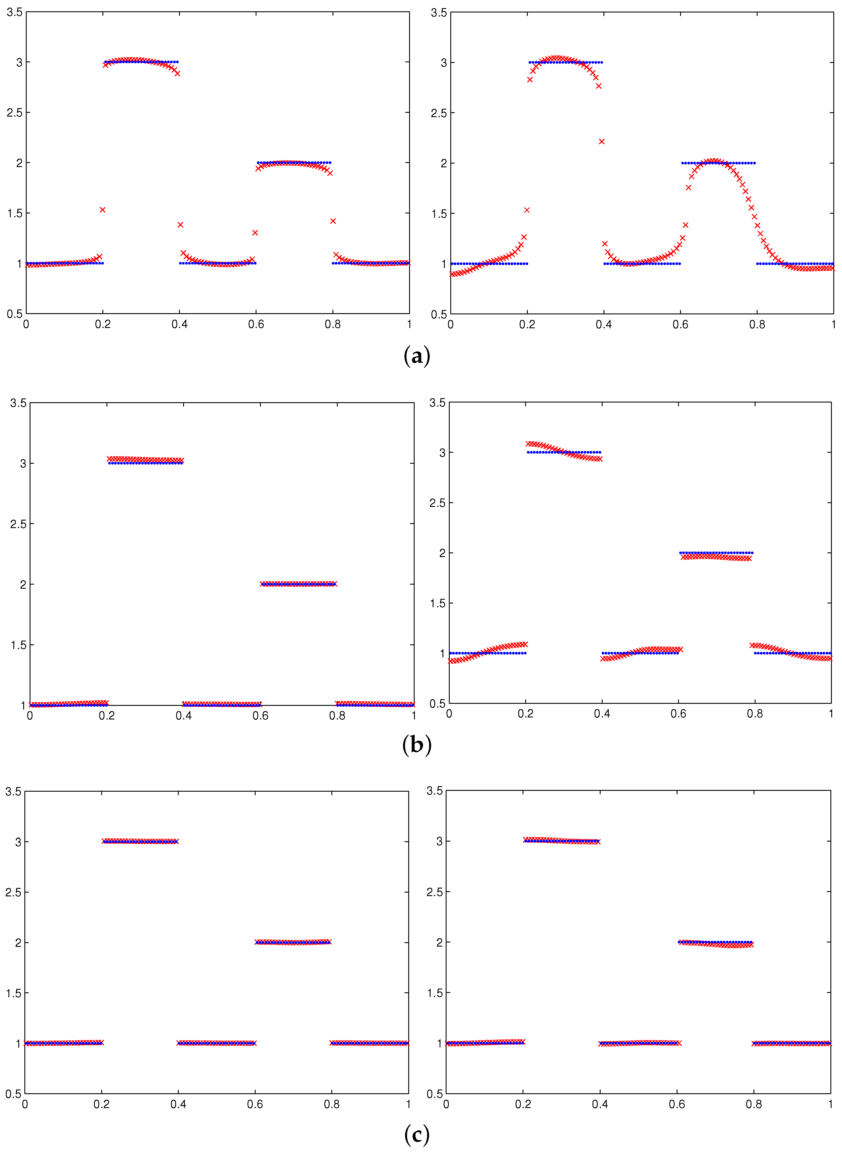
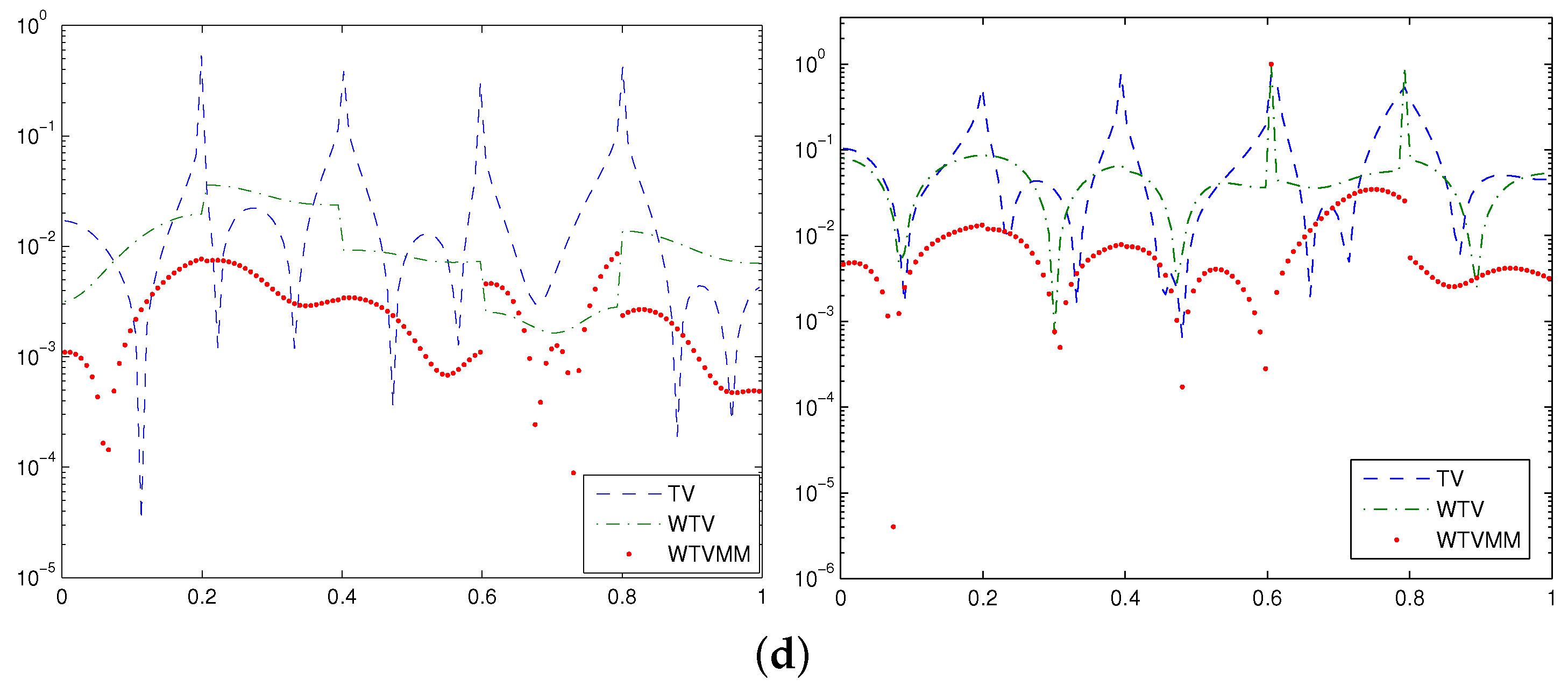
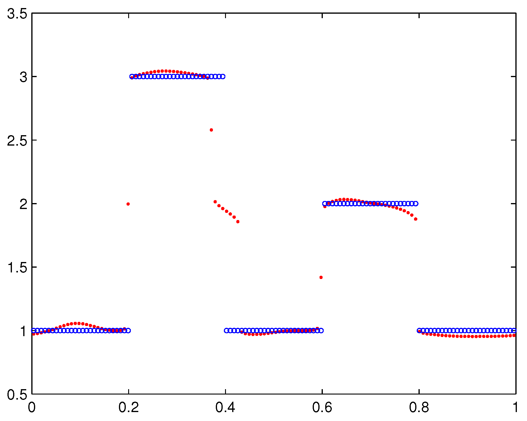
Figure 2. The exact solution (dot), numerical solutions (x) and point-wise errors for the three methods for Example 1 with noisy right-hand sides containing $1\%$ (left) and $10\%$ (right) of white noise. (a) Numerical solutions of TV; (b) numerical solutions of WTV; (c) numerical solutions of WTVMM; and (d) point-wise errors of the numerical solutions.

Table 1. Parameters used, number of iterations and relative errors for different methods for Example 1 where the right-hand side contains 1% of white noise. TV: total variation; WTV: weighted total variation; WTVMM: weighted total variation Modica-Mortola.

	$(\mathit{\alpha },\mathit{\beta },\mathit{\theta },\mathit{\gamma })$	$\#\mathit{it}$	Error
TV	($5.0\times {10}^{-2}$, $2.5\times {10}^{-5}$, -, -)	24	$4.5\times {10}^{-2}$
WTV	($5.0\times {10}^{-2}$, $2.5\times {10}^{-5}$, $5.0\times {10}^{-2}$, -)	11	$8.61\times {10}^{-3}$
WTVMM	($5.0\times {10}^{-2}$, $2.5\times {10}^{-5}$, $5.0\times {10}^{-2}$, 1)	11 + 4	$1.98\times {10}^{-3}$

Table 2. Parameters used, number of iterations and relative errors for different methods for Example 1 where the noisy right-hand side contains 10% of white noise.

	$(\mathit{\alpha },\mathit{\beta },\mathit{\theta },\mathit{\gamma })$	$\#\mathit{it}$	Error
TV	($1.0\times {10}^{-1}$, $5.0\times {10}^{-5}$, -, -)	10	$9.48\times {10}^{-2}$
WTV	($1.0\times {10}^{-1}$, $5.0\times {10}^{-3}$, $5.0\times {10}^{-2}$, -)	13	$7.18\times {10}^{-2}$
WTVMM	($1.0\times {10}^{-1}$, $5.0\times {10}^{-2}$, $5.0\times {10}^{-2}$, 1)	10+11	$5.03\times {10}^{-2}$

We have tried a one-stage method for solving Example 1. The best numerical solution we obtained by minimizing the function $\frac{1}{2}J\left(\mathbf{f}\right)+\alpha {\mathrm{TV}}_{1,\beta }\left(\mathbf{f}\right)+\frac{\gamma }{2}\mathrm{M}\left(\mathbf{f}\right)$ for Example 1 is shown in Figure 3. We observe from all figures in Figure 2 and Figure 3 that the numerical solution obtained via the WTVMM method is the best.

Figure 3. The exact solution (circle) and the numerical solution obtained by minimizing $\frac{1}{2}J\left(\mathbf{f}\right)+\alpha {\mathrm{TV}}_{1,\beta }\left(\mathbf{f}\right)+\gamma \mathrm{M}\left(\mathbf{f}\right)$ (dot) for Example 1 where the noisy right-hand side contains $10\%$ of white noise.

We make the following remarks based on the above numerical results.

(1)

For the WTVMM method, the main cost lies in obtaining the numerical solution ${\mathbf{f}}_{\mathbf{TV}}^{*}$, i.e., minimization of ${\mathsf{\Phi }}_{\mathrm{TV}}\left(\mathbf{f}\right)$ defined by (8).

(2)

The numerical solutions obtained by using the WTV method are better than those obtained by the TV method. The numerical solutions obtained by using the WTVMM method can be quite accurate, which can be clearly seen from the relative errors shown in Table 1 and Table 2, the numerical solutions shown in Figure 2c and the point-wise errors shown in Figure 2d.

(3)

If the position of the break points in the solution can be identified by the previous step, the approximate solution obtained by the WTVMM method can be very accurate. In the other hand, since the local minimizer of ${\mathsf{\Phi }}_{\mathrm{M}}$ obtained by the DN method is sensitive to the initial guess, we may not be able to obtain a good numerical solution if the approximate solution obtained in the previous step cannot identify the break points well.

To demonstrate the influence of the values of parameters on numerical solutions, we present the relative errors of the numerical solutions of the three methods for a considerably different set of the parameter combinations $(\beta ,\theta )$ in Table 3 and Table 4. We can see from the tables that if the values of the parameters are not too far from the optimal ones, we can obtain satisfactory numerical solutions. Moreover, both values of β and θ affect the quality of the numerical solutions, and a correct choice of β seems more important (see the column corresponding to $\beta =2.5\times {10}^{-3}$ in Table 3 and the one for $\beta =2.5\times {10}^{-2}$ in Table 4). Moreover, we can see that satisfying numerical solutions can be obtained by using different parameter combinations.

Table 3. Relative errors for TV (1st element), WTV (2nd element) and WTVMM (3rd element) with different β and θ for Example 1 with the right-hand side containing 1% of white noise.

	$\mathit{\beta }$	$2.5\times {10}^{-3}$	$2.5\times {10}^{-4}$	$2.5\times {10}^{-6}$
$\mathit{\theta }$
5.0		($1.05\times {10}^{-1}$, $4.82\times {10}^{-2}$, $4.88\times {10}^{-2}$)	($5.74\times {10}^{-2}$, $4.70\times {10}^{-2}$, $4.89\times {10}^{-2}$)	($4.67\times {10}^{-2}$, $4.88\times {10}^{-2}$, $4.89\times {10}^{-2}$)
$5.0\times {10}^{-1}$		($1.05\times {10}^{-1}$, $1.73\times {10}^{-2}$, $1.98\times {10}^{-3}$)	($5.74\times {10}^{-2}$, $1.30\times {10}^{-2}$, $1.98\times {10}^{-3}$)	($4.67\times {10}^{-2}$, $9.51\times {10}^{-3}$, $1.98\times {10}^{-3}$)
$5.0\times {10}^{-3}$		($1.05\times {10}^{-1}$, $1.05\times {10}^{-2}$, $1.98\times {10}^{-3}$)	($5.74\times {10}^{-2}$, $3.28\times {10}^{-2}$, $4.94\times {10}^{-2}$)	($4.67\times {10}^{-2}$, $1.42\times {10}^{-1}$, $1.30\times {10}^{-1}$)

Table 4. Relative errors for TV (1st element), WTV (2nd element) and WTVMM (3rd element) with different β and θ for Example 1 with the right-hand side containing 10% of white noise.

	$\mathit{\beta }$	$5.0\times {10}^{-1}$	$5.0\times {10}^{-2}$	$5.0\times {10}^{-4}$
$\mathit{\theta }$
$5.0\times {10}^{-1}$		($1.48\times {10}^{-1}$, $1.46\times {10}^{-1}$, $1.49\times {10}^{-1}$)	($1.49\times {10}^{-1}$, $8.93\times {10}^{-2}$, $7.09\times {10}^{-2}$)	($9.48\times {10}^{-2}$, $8.37\times {10}^{-2}$, $8.59\times {10}^{-2}$)
$5.0\times {10}^{-3}$		($1.48\times {10}^{-1}$, $1.46\times {10}^{-1}$, $1.93\times {10}^{-1}$)	($1.49\times {10}^{-1}$, $8.56\times {10}^{-2}$, $5.03\times {10}^{-2}$)	($9.48\times {10}^{-2}$, $1.21\times {10}^{-1}$, $1.22\times {10}^{-1}$)
$5.0\times {10}^{-4}$		($1.48\times {10}^{-1}$, $1.47\times {10}^{-1}$, $1.79\times {10}^{-1}$)	($1.49\times {10}^{-1}$, $8.56\times {10}^{-2}$, $5.03\times {10}^{-2}$)	($9.48\times {10}^{-2}$, $1.31\times {10}^{-1}$, $1.31\times {10}^{-1}$)

Example 2.

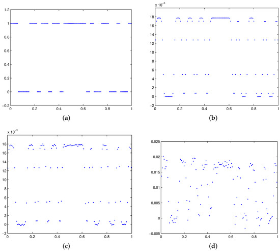
(Barcode reading) The Fredholm integral equation can serve as a good approximation of the blurring inside a barcode reader ([1], p. 135). The kernel of the equation is given by:

$$k(x,t)=e^{-\frac{{(x-t)}^2}{{\sigma }^2}}.$$

In our numerical tests, we choose $\sigma =0.01$. The intensity of the printed barcode and the exact right-hand side are shown in Figure 4a,b, and two noisy right-hand sides are shown in Figure 4c,d, respectively.

Figure 4. The exact solution, the right-hand side, and noisy right-hand sides for Example 2. (a) The exact solution; (b) the right-hand side; (c) a noisy right-hand side containing $1\%$ of white noise; and (d) a noisy right-hand side containing $10\%$ of white noise.

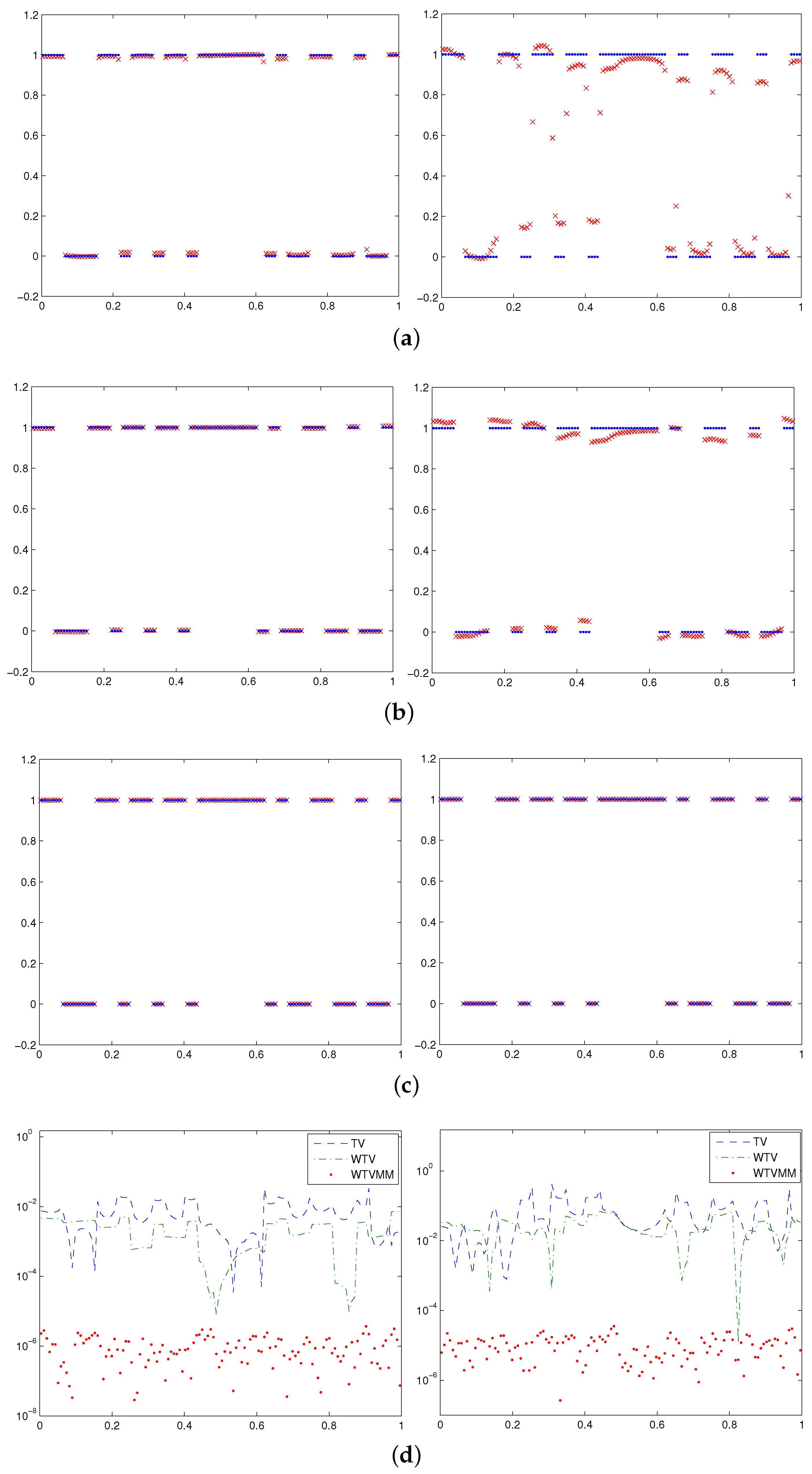
Since the average of $c_1$ and $c_2$ is $0.5$, we choose ${\mathbf{f}}_0={(0.5,0.5,\dots ,0.5)}^T$ as initial guess for minimization of the functions corresponding to the TV and WTV functionals. Numerical solutions obtained by different methods, as well as the the point-wise error for all numerical solutions are shown in Figure 5. The relevant parameters, the number of iterations and the relative errors are given in Table 5 and Table 6.

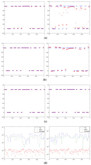
Figure 5. The exact solution (dot), numerical solutions (x) and point-wise errors for the three methods for Example 2 with noisy right-hand sides containing $1\%$ (left) and $10\%$ (right) of white noise. (a) Numerical solutions of TV; (b) numerical solutions of WTV; (c) numerical solutions of WTVMM; and (d) point-wise errors of the numerical solutions.

Table 5. Parameters used, number of iterations and relative errors for different methods for Example 2 where the right-hand side contains 1% of white noise.

	$(\mathit{\alpha },\mathit{\beta },\mathit{\theta },\mathit{\gamma })$	$\#\mathit{it}$	Error
TV	($5.0\times {10}^{-6}$, $2.5\times {10}^{-5}$, -, -)	14	$1.13\times {10}^{-2}$
WTV	($5.0\times {10}^{-6}$, $2.5\times {10}^{-5}$, $5.0\times {10}^{-2}$, -)	8	$3.79\times {10}^{-3}$
WTVMM	($5.0\times {10}^{-6}$, $2.5\times {10}^{-5}$, $5.0\times {10}^{-2}$, 1)	8+3	$1.65\times {10}^{-6}$

Table 6. Parameters used, number of iterations and relative errors for different methods for Example 2 where the right-hand side contains 10% of white noise.

	$(\mathit{\alpha },\mathit{\beta },\mathit{\theta },\mathit{\gamma })$	$\#\mathit{it}$	Error
TV	($4.0\times {10}^{-5}$, $1.0\times {10}^{-4}$, -, -)	16	$1.29\times {10}^{-1}$
WTV	($4.0\times {10}^{-5}$, $2.5\times {10}^{-3}$, $5.0\times {10}^{-2}$, -)	11	$4.14\times {10}^{-2}$
WTVMM	($4.0\times {10}^{-5}$, $2.5\times {10}^{-3}$, $5.0\times {10}^{-2}$, 1)	11+4	$1.65\times {10}^{-5}$

Again, from Figure 5 and Table 5 and Table 6, one can observe that the numerical solutions obtained by using the WTVMM method are much better than those obtained by using the TV and WTV methods. In fact, we can obtain an approximate barcode of very high quality by using the WTVMM method.

5. Concluding Remarks

We presented a two-stage numerical method for estimating piecewise-constant solutions for Fredholm integral equations of the first kind. The main work of the two-stage method is the minimization of ${\mathsf{\Phi }}_{\mathrm{TV}}\left(\mathbf{f}\right)$, which may require many iterations. Numerical results showed that if the relevant parameters are chosen suitably, the proposed method can obtain satisfying numerical solutions. We will study regularization parameter choosing methods, as well as efficient algorithms for relevant minimization problems for weighted total variation (WTV) methods, including iterative scheme for parameter determination.

References

- Hansen, P.C. Discrete Inverse Problems: Insight and Algorithms; SIAM: Philadelphia, PA, USA, 2010. [Google Scholar]
- Delves, L.M.; Mohamed, J.L. Computational Methods for Integral Equations; Cambridge University Press: Cambridge, UK, 1985. [Google Scholar]
- Dehghan, M.; Saadatmandi, A. Chebyshev finite difference method for Fredholm integro-differential equation. Int. J. Comput. Math. 2008, 85, 123–130. [Google Scholar]
- Ghasemi, M.; Babolian, E.; Kajani, M.T. Numerical solution of linear Fredholm integral equations using sinecosine wavelets. Int. J. Comput. Math. 2007, 84, 979–987. [Google Scholar]
- Koshev, N.; Beilina, L. An adaptive finite element method for Fredholm integral equations of the first kind and its verification on experimental data. CEJM 2013, 11, 1489–1509. [Google Scholar]
- Koshev, N.; Beilina, L. A posteriori error estimates for Fredholm integral equations of the first kind. In Applied Inverse Problems, Springer Proceedings in Mathematics and Statistics; Springer: New York, NY, USA, 2013; Volume 48, pp. 75–93. [Google Scholar]
- Zhang, Y.; Lukyanenko, D.V.; Yagola, A.G. Using Lagrange principle for solving linear ill-posed problems with a priori information. Numer. Methods Progr. 2013, 14, 468–482. (In Russian) [Google Scholar]
- Vogel, C.R. Computational Methods for Inverse Problems; SIAM: Philadelphia, PA, USA, 2002. [Google Scholar]
- Tikhonov, A.N. Regularization of incorrectly posed problems. Sov. Math. Dokl. 1964, 4, 1624–1627. [Google Scholar]
- Hansen, P.C. The truncated SVD as a method for regularization. BIT Numer. Math. 1987, 27, 534–553. [Google Scholar]
- Hansen, P.C.; Sekii, T.; Shibahashi, H. The modified truncated SVD method for regularization in general form. SIAM J. Sci. Stat. Comput. 1992, 13, 1142–1150. [Google Scholar]
- Rashed, M.T. Numerical solutions of the integral equations of the first kind. Appl. Math. Comput. 2003, 145, 413–420. [Google Scholar]
- Lin, S.; Cao, F.; Xu, Z. A convergence rate for approximate solutions of Fredholm integral equations of the first kind. Positivity 2012, 16, 641–652. [Google Scholar]
- Wang, K.; Wang, Q. Taylor collocation method and convergence analysis for the Volterra-Fredholm integral equations. J. Comput. Appl. Math. 2014, 260, 294–300. [Google Scholar]
- Neggal, B.; Boussetila, N.; Rebbani, F. Projected Tikhonov regularization method for Fredholm integral equations of the first kind. J. Inequal. Appl. 2016. [Google Scholar]
- Rudin, L.I.; Osher, S.; Fatemi, E. Nonlinear total variation based noise removal algorithms. Physica 1992, 60, 259–268. [Google Scholar]
- Acar, R.; Vogel, C.R. Analysis of bounded variation penalty methods for ill-posed problems. Inverse Probl. 1994, 10, 1217–1229. [Google Scholar]
- Wang, Y.; Yang, J.; Yin, W.; Zhang, Y. A new alternating minimization algorithm for total variation image reconstruction. SIAM J. Imaging Sci. 2008, 1, 248–272. [Google Scholar]
- Defrise, M.; Vanhove, C.; Liu, X. An algorithm for total variation regularization in high-dimensional linear problems. Inverse Probl. 2011, 27, 065002. [Google Scholar]
- Fadili, J.M.; Peyré, G. Total variation projection with first order schemes. IEEE Trans. Image Process. 2011, 20, 657–669. [Google Scholar]
- Micchelli, C.A.; Shen, L.; Xu, Y. Proximity algorithms for image models: Denoising. Inverse Probl. 2011, 27, 045009. [Google Scholar]
- Chan, R.H.; Liang, H.X.; Ma, J. Positively constrained total variation penalized image restoration. Adv. Adapt. Data Anal. 2011, 3, 1–15. [Google Scholar]
- Strong, D.M.; Blomgren, P.; Chan, T.F. Spatially adaptive local feature-driven total variation minimizing image restoration. Proc. SPIE 1997, 222–233. [Google Scholar]
- Chantas, G.; Galatsanos, N.P.; Molina, R.; Katsaggelos, A.K. Variational Bayesian image restoration with a product of spatially weighted total variation image priors. IEEE Trans. Image Process. 2010, 19, 351–362. [Google Scholar]
- Chen, Q.; Montesinos, P.; Sun, Q.S.; Heng, P.A.; Xia, D.S. Adaptive total variation denoising based on difference curvature. Image Vision Comput. 2010, 28, 298–306. [Google Scholar]
- Chopra, A.; Lian, H. Total variation, adaptive total variation and nonconvex smoothly clipped absolute deviation penalty for denoising blocky images. Pattern Recognit. 2010, 43, 2609–2619. [Google Scholar]
- El Hamidi, A.; Ménard, M.; Lugiez, M.; Ghannam, C. Weighted and extended total variation for image restoration and decomposition. Pattern Recognit. 2010, 43, 1564–1576. [Google Scholar]
- Hansen, P.C.; Mosegaard, K. Piecewise polynomial solutions to linear inverse problems. Lect. Notes Earth Sci. 1996, 63, 284–294. [Google Scholar]
- Jin, B.T.; Zou, J. Numerical estimation of piecewise constant Robin coefficient. SIAM J. Control Optim. 2009, 48, 1977–2002. [Google Scholar]
- Bogosel, B.; Oudet, É. Qualitative and numerical analysis of a spectral problem with perimeter constraint. SIAM J. Control Optim. 2016, 54, 317–340. [Google Scholar]
- Chan, R.H.; Ng, M.K. Conjugate gradient method for Toeplitz systems. SIAM Rev. 1996, 38, 427–482. [Google Scholar]
- Groetsch, C.W. Integral equations of the first kind, inverse problems and regularization: A crash course. J. Phys. Conf. Ser. 2007, 73, 012001. [Google Scholar]
- Goncharskii, A.V.; Leonov, A.S.; Yagola, A.G. A generalized discrepancy principle. USSR Comput. Math. Math. Phys. 1973, 13, 25–37. [Google Scholar]
- Bakushinsky, A.; Kokurin, M.Y.; Smirnova, A. Iterative Methods for Ill-posed Problems: An Introduction. Inverse and Ill-Posed Problems Series 54. De Gruyter: Berlin, Germany; New York, NY, USA, 2011. [Google Scholar]
© 2017 by the authors. Licensee MDPI, Basel, Switzerland. This article is an open access article distributed under the terms and conditions of the Creative Commons Attribution (CC BY) license (http://creativecommons.org/licenses/by/4.0/).