SIC-POVMs and Compatibility among Quantum States

Abstract

An unexpected connection exists between compatibility criteria for quantum states and Symmetric Informationally Complete quantum measurements (SIC-POVMs). Beginning with Caves, Fuchs and Schack’s "Conditions for compatibility of quantum state assignments", I show that a qutrit SIC-POVM studied in other contexts enjoys additional interesting properties. Compatibility criteria provide a new way to understand the relationship between SIC-POVMs and mutually unbiased bases, as calculations in the SIC representation of quantum states make clear. This, in turn, illuminates the resources necessary for magic-state quantum computation, and why hidden-variable models fail to capture the vitality of quantum mechanics.

1. A Compatibility Criterion for Quantum States

This article presents an unforeseen connection between two subjects originally studied for separate reasons by the Quantum Bayesians, or to use the more recent and specific term, QBists [1,2]. One of these topics originates in the paper “Conditions for compatibility of quantum state assignments” [3] by Caves, Fuchs and Schack (CFS). Refining CFS’s treatment reveals an unexpected link between the concept of compatibility and other constructions of quantum information theory.

We begin by taking up the question of what it means for probability distributions to be compatible with one another. Consider a thoroughly classical scenario, in which Alice and Bob are gambling on the outcome of a coin toss. Both Alice and Bob are certain the toss is rigged, but Alice is convinced that the outcome will be heads, while Bob is equally steadfast in maintaining that it will be tails. That is, $p_A\left(H\right)=1$ and $p_A\left(T\right)=0$, while $p_B\left(H\right)=0$ and $p_B\left(T\right)=1$. No matter which way the coin lands, one party will be disappointed—or, depending on the stakes, bankrupt.

We can equally well present a single-user version of this scenario. Imagine that Alice, and only Alice, is gambling on the coin flip, and that conditional on some other information, she will choose to do so in accordance with either the probability distribution

$$p_A\left(H\right)=1,p_A\left(T\right)=0$$

(1)

or the alternative,

$$p_A^{\prime }\left(H\right)=0,p_A^{\prime }\left(T\right)=1$$

(2)

For example, Alice may be confident that the toss will be rigged and that she can deduce which way it will be rigged once she can observe the handedness of the coin-tosser. The incompatibility between $p_A$ and $p_A^{\prime }$ is then relevant to Alice, regardless of the presence or absence of other players.

Having formulated the scenario in single-user terms, we can develop a quantum analogue; a single-user statement avoids the conceptual problem of whether an event occurring for an agent Alice could, in the quantum setting, itself be an event for any other agent [2]. The quantum version of this kind of incompatibility is a condition on pairs of quantum states. Take two density matrices ${\rho }_A$ and ${\rho }_A^{\prime }$. If there exists a measurement $\left\{E_i\right\}$ such that

$$\sum _i\text{tr}\left({\rho }_A{E}_i\right)\text{tr}\left({\rho }_A^{\prime }{E}_i\right)=0$$

(3)

then ${\rho }_A$ and ${\rho }_A^{\prime }$ are called post-Peierls incompatible [3]. If two states are post-Peierls (PP) compatible, then for all experiments, there is at least one outcome for which both states yield nonzero probability via the Born rule. We can naturally extend this criterion to sets of more than two quantum states. In general, a set of N states is PP incompatible when, for some experiment $\left\{E_i\right\}$,

$$\sum _i\prod _{a=1}^N\text{tr}({\rho }^{\left(a\right)}{E}_i)=0$$

(4)

A von Neumann measurement is a Positive Operator Valued Measure (POVM) with d possible outcomes, specified by a set of d orthonormal vectors in Hilbert space. In terms of projection operators, each von Neumann measurement comprises d one-dimensional orthogonal projectors. We abbreviate this phrase as ODOP. Therefore, compatibility with respect to von Neumann measurements is known as PP-ODOP compatibility [3]. When we formulate an exact criterion for PP-ODOP compatibility of qutrit pure states, i.e., pure states in $d=3$, we find something interesting.

In the next two sections, we will examine PP-ODOP compatibility in more detail and find a connection to another topic of much interest to the QBist research program. For completeness, we note that compatibility criteria have also recently entered the quantum foundations discourse through a different route. They play a key role in discussions of whether quantum states can be treated as encoding information about the values of hidden variables [4,5]. In this paper, we disregard the issue of hidden variables and treat quantum states as directly specifying the probabilities of experiment outcomes.

2. Three Pure States in Dimension Three

It is possible to have triplets of states which are PP-ODOP incompatible when taken all together, even though they are compatible when taken in pairs. CFS provide a specific example, which for convenience we reproduce here. Pick an orthonormal basis $\{\left|0\right.〉,\left|1\right.〉,\left|2\right.〉\}$, and consider the following three possible states which can be ascribed to a qutrit:

$$\begin{array}{cc}\hfill \left|\psi \right.〉& =\frac{1}{\sqrt{2}}\left(\left|1\right.〉+\left|2\right.〉\right)\hfill \\ \hfill \left|{\psi }^{\prime }\right.〉& =\frac{1}{\sqrt{2}}\left(\left|2\right.〉+\left|0\right.〉\right)\hfill \\ \hfill \left|{\psi }^{″}\right.〉& =\frac{1}{\sqrt{2}}\left(\left|0\right.〉+\left|1\right.〉\right)\hfill \end{array}$$

(5)

Now, Alice the graduate student performs a von Neumann experiment in the computational basis of $\{\left|0\right.〉,\left|1\right.〉,\left|2\right.〉\}$. Whatever result she experiences, there is a state assignment in the set $\{\left|\psi \right.〉,\left|{\psi }^{\prime }\right.〉,\left|{\psi }^{″}\right.〉\}$ according to which that experience is an event of probability zero.

By pursuing this argument, we will have the opportunity, incidentally, to correct two mathematical errors in CFS. Both are slight, but one is a missed opportunity, as it introduced an inconsistency into CFS’s calculations and obscured the connection which we shall examine here.

A general set of three pure states $\{\left|\psi \right.〉,\left|{\psi }^{\prime }\right.〉,\left|{\psi }^{″}\right.〉\}$ is PP-ODOP incompatible at the tertiary level if some orthonormal basis $\{\left|0\right.〉,\left|1\right.〉,\left|2\right.〉\}$ exists such that

$$\begin{array}{cc}\hfill \left|\psi \right.〉& =e^{i\chi }\left(cos\theta \left|1\right.〉+e^{i\varphi }sin\theta \left|2\right.〉\right)\hfill \\ \hfill \left|{\psi }^{\prime }\right.〉& =e^{i{\chi }^{\prime }}\left(cos{\theta }^{\prime }\left|2\right.〉+e^{i{\varphi }^{\prime }}sin{\theta }^{\prime }\left|0\right.〉\right)\hfill \\ \hfill \left|{\psi }^{″}\right.〉& =e^{i{\chi }^{″}}\left(cos{\theta }^{″}\left|0\right.〉+e^{i{\varphi }^{″}}sin{\theta }^{″}\left|1\right.〉\right)\hfill \end{array}$$

(6)

The three θ angles are restricted to the interval $(0,\pi /2)$, while the χ and $\varphi$ angles must all lie in the interval $[0,2\pi )$. Taking the inner products picks out one basis vector per pair:

$$\begin{array}{cc}\hfill 〈\psi |{\psi }^{\prime }〉& =e^{i({\chi }^{\prime }-\chi )}{e}^{-i\varphi }sin\theta cos{\theta }^{\prime }\hfill \\ \hfill 〈{\psi }^{\prime }|{\psi }^{″}〉& =e^{i({\chi }^{″}-{\chi }^{\prime })}{e}^{-i{\varphi }^{\prime }}sin{\theta }^{\prime }cos{\theta }^{″}\hfill \\ \hfill 〈{\psi }^{″}|\psi 〉& =e^{i(\chi -{\chi }^{″})}{e}^{-i{\varphi }^{″}}sin{\theta }^{″}cos\theta \hfill \end{array}$$

(7)

This is the first of the two errata mentioned above: because the $\varphi$-dependent phase factors come from the bra vectors rather than the ket vectors, the sign in the exponential should be negative, instead of positive as written in CFS’s Equation (19). The sign error cancels in the next step, which is to multiply these quantities by their complex conjugates, yielding

$$\begin{array}{cc}\hfill {\left|〈\psi |{\psi }^{\prime }〉\right|}^2& ={sin}^2\theta {cos}^2{\theta }^{\prime }\hfill \\ \hfill {\left|〈{\psi }^{\prime }|{\psi }^{″}〉\right|}^2& ={sin}^2{\theta }^{\prime }{cos}^2{\theta }^{″}\hfill \\ \hfill {\left|〈{\psi }^{″}|\psi 〉\right|}^2& ={sin}^2{\theta }^{″}{cos}^2\theta \hfill \end{array}$$

(8)

After some algebra, one can prove from Equation (8) that three pure states in $d=3$ are PP-ODOP incompatible if and only if

$$\begin{array}{cc}\hfill {\left|〈\psi |{\psi }^{\prime }〉\right|}^2+{\left|〈{\psi }^{\prime }|{\psi }^{″}〉\right|}^2+{\left|〈{\psi }^{″}|\psi 〉\right|}^2& <1\hfill \end{array}$$

(9)

$$\begin{array}{cc}\hfill {\left({\left|〈\psi |{\psi }^{\prime }〉\right|}^2+{\left|〈{\psi }^{\prime }|{\psi }^{″}〉\right|}^2+{\left|〈{\psi }^{″}|\psi 〉\right|}^2-1\right)}^2& \ge 4{\left|〈\psi |{\psi }^{\prime }〉\right|}^2{\left|〈{\psi }^{\prime }|{\psi }^{″}〉\right|}^2{\left|〈{\psi }^{″}|\psi 〉\right|}^2\hfill \end{array}$$

(10)

This is the second glitch in CFS: the latter inequality should be ≥ rather than >, as written in CFS’s Formula (28). This is the more consequential error, since if the inequality is strict, then the example of three-party PP-incompatible states which CFS provide—our triplet Equation (5)—is not consistent with CFS’s compatibility criterion.

3. Qutrit SIC POVMs

The second inequality has a more intricate structure than the first. What happens when we try to saturate it? Suppose we require that the three squared overlaps all have the same value, x. Then, saturating the second inequality implies that x satisfies the cubic equation

$$4x^3-9x^2+6x-1=0$$

(11)

This cubic polynomial has a zero at $x=\frac{1}{4}$, and a double zero at $x=1$, which is disallowed by the requirement that the states are nonidentical.

How many states can we push simultaneously to the edge of PP-ODOP incompatibility in this way? That is, how many states in qutrit state space can we find such that for any two of them,

$${\left|〈{\psi }_i|{\psi }_j〉\right|}^2=\frac{1+3{\delta }_{ij}}{4}$$

(12)

This is the problem of finding the maximal set of equiangular lines in three-dimensional complex vector space.

Beginning with the question of compatibility among probability distributions, we have arrived at Symmetric Informationally Complete POVMs [2,6,7,8,9]. This term is abbreviated to SIC-POVM, or just to SIC (pronounced like “seek”). A SIC for a d-dimensional Hilbert space is a set of $d^2$ operators $\{E_i=\frac{1}{d}{\Pi }_i\}$ where the rank-one projection operators $\left\{{\Pi }_i\right\}$ satisfy

$$\text{tr}\left({\Pi }_k{\Pi }_l\right)=\frac{d{\delta }_{kl}+1}{d+1}$$

(13)

It is known that SICs are maximal in this regard, i.e., no more than $d^2$ operators can simultaneously satisfy Equation (13). For qutrits, this means that a set of states such that any three saturate the edge of PP-ODOP incompatibility can contain at most nine states.

We have shown that any triple of states chosen from a qutrit SIC will be PP-incompatible. One might expect that a large number of different von Neumann measurements would be required to cover all the possible choices of triples, perhaps comparable to the number of triples themselves. Surprisingly, this is not the case; our toolbox can be much more economical. Take $\omega =e^{2\pi i/3}$, and construct the set of states $\left\{\left|{\psi }_j\right.〉\right\}$ given by the columns of the following matrix:

$$\frac{1}{\sqrt{2}}\left(\begin{array}{ccccccccc}0& -1& 1& 0& -1& 1& 0& -1& 1\\ 1& 0& -1& \omega & 0& -\omega & {\omega }^2& 0& -{\omega }^2\\ -1& 1& 0& -{\omega }^2& {\omega }^2& 0& -\omega & \omega & 0\end{array}\right)$$

(14)

The set of nine states $\left\{\left|{\psi }_i\right.〉\right\}$ forms a SIC known as the Hesse SIC [10]. For the Hesse SIC, a set of four orthogonal bases is sufficient to reveal the PP-incompatibility of all possible triples. Moreover, the requisite bases have an interesting property: they are mutually unbiased with respect to each other. In general, two bases are mutually unbiased if, for any vector $\left|\psi \right.〉$ in one basis and any vector $\left|\varphi \right.〉$ in the other, $|〈\psi |\varphi 〉{|}^2=1/d$. Any set of three states drawn from the SIC will be revealed as PP-incompatible by a measurement in one or more of the Mutually Unbiased Bases (MUB). We construct each basis vector by finding a state orthogonal to three of the SIC states. Specifically, each basis vector corresponds to an element in a Steiner triple system [11] of order 9, which we build by cyclically tracing all the horizontal, vertical and diagonal lines in the array

$$\begin{array}{ccc}0& 1& 2\\ 3& 4& 5\\ 6& 7& 8\end{array};\text{that}\text{is}\text{to}\text{say},S\left(9\right)=\begin{array}{ccc}\left(012\right)& \left(345\right)& \left(678\right)\\ \left(036\right)& \left(147\right)& \left(258\right)\\ \left(048\right)& \left(156\right)& \left(237\right)\\ \left(057\right)& \left(138\right)& \left(246\right)\end{array}$$

(15)

Each possible value of the index i occurs in exactly four entries of $S\left(9\right)$, and each possible pair of index values occurs exactly once. It is easiest to see the meaning of this construction using the SIC representation of quantum states. Any quantum state, pure or mixed, is equivalent to a probability distribution over the outcomes of an informationally complete measurement, and the qutrit SIC of Equation (14) furnishes such a measurement. An arbitrary qutrit density matrix ρ can be decomposed as

$$\rho =\sum _{i=0}^8\left(4p\left(i\right)-\frac{1}{3}\right){\Pi }_i=4\sum _{i=0}^{8}p\left(i\right){\Pi }_i-I$$

(16)

where ${\Pi }_i=\left|{\psi }_i\right.〉\left.〈{\psi }_i\right|$ and $p\left(i\right)$ is the Born-rule probability

$$p\left(i\right)=\frac{1}{3}\text{tr}\left(\rho {\Pi }_i\right)$$

(17)

To construct the state orthogonal to SIC vectors $\left|{\psi }_i\right.〉$, $\left|{\psi }_j\right.〉$ and $\left|{\psi }_k\right.〉$, we simply write a probability vector $\mathbf{p}$ which is zero in entries i, j and k, and $\frac{1}{6}$ everywhere else.

To see why this construction yields a complete set of MUB, we use the fact that the Hilbert–Schmidt inner product of density matrices is just an affine transformation of the Euclidean inner product of the corresponding probability distributions [2,12]. For qutrit states,

$$\text{tr}\rho \sigma =12\mathbf{p}·\mathbf{q}-1$$

(18)

This means that if ρ and σ are orthogonal, then $\mathbf{p}·\mathbf{q}=1/12$.

With this, we can see that the vectors orthogonal to $\left(012\right)$ and $\left(345\right)$, for example, must be orthogonal to each other, because when we take the dot product of their SIC representations, we only have three nonzero contributions. If instead we take the vectors orthogonal to $\left(012\right)$ and $\left(036\right)$, say, a zero in one vector coincides with a zero in the other, the dot product can come out larger. These within-row and between-rows relationships hold generally. Each row corresponds to a set of three mutually orthogonal vectors, and when we take vectors from two different rows, we always get the same nonzero overlap: the Hilbert space inner product of their density matrices is always $\frac{1}{3}$.

We have fashioned a complete set of mutually unbiased bases. Starting with the SIC Equation (14), we constructed 12 pure states which fall into four sets of three. Each set of three, corresponding to a row in our table, is an orthonormal basis. When we take the Hilbert–Schmidt inner product of a state from one basis with a state from another, we get $1/3$ every time. This is the requirement for two bases to be mutually unbiased in $d=3$ (in older language, the observables associated with any two such bases are complementary [13]). Furthermore, the largest number of MUB that can exist in d dimensions is $d+1$ [14], and we constructed four. From now on, we will refer to these $d(d+1)=12$ vectors as MUB states for short. While the relation between qutrit SIC and MUB states has been known for some time [10,15], the convenience of the SIC representation has so far not been appreciated.

Given any three distinct elements from the SIC set, a measurement in at least one of the MUB will reveal PP-ODOP incompatibility among those three states. For example, say we pick the SIC elements $\left|{\psi }_0\right.〉$, $\left|{\psi }_1\right.〉$ and $\left|{\psi }_4\right.〉$. Then, we measure in the basis given by the vectors orthogonal to the fourth row: $\left(057\right)$, $\left(138\right)$, $\left(246\right)$. Each possible outcome of the experiment conflicts with one of the three given states: the first with the state ascription $\left|{\psi }_0\right.〉$, the second with the ascription $\left|{\psi }_1\right.〉$ and the third with $\left|{\psi }_4\right.〉$. Therefore, we have PP-ODOP incompatibility at the ternary level, while of course any two distinct states in the SIC are pairwise compatible, having an inner-product-squared of $1/(d+1)=1/4$.

Note that the second error in CFS, writing > instead of ≥ in the condition Equation (10), mistakenly implies that triplets of SIC states are PP-ODOP compatible, though barely so. This is clearly incorrect, as we can see by testing $\left|{\psi }_0\right.〉$, $\left|{\psi }_1\right.〉$ and $\left|{\psi }_2\right.〉$ in the computational basis.

4. Additional Properties of the Hesse SIC and Associated MUB

In order to be a SIC representation of a pure quantum state, a probability distribution $p\left(i\right)$ must satisfy two conditions [2]. The first is quadratic:

$$\sum _{i}p{\left(i\right)}^2=\frac{2}{d(d+1)}$$

(19)

and the second is cubic, or “QBic”:

$$\sum _{ijk}\text{Re}\left[\text{tr}\left({\Pi }_i{\Pi }_j{\Pi }_k\right)\right]p\left(i\right)p\left(j\right)p\left(k\right)=\frac{d+7}{{(d+1)}^3}$$

(20)

The quadratic condition has an interesting interpretation that provides a handy mnemonic for it [16].

Whenever we have a probability distribution, we can compute indices that summarize its properties. One well-known example is the Shannon entropy, also designated as the Shannon information or Shannon index, which reflects the extent to which a probability distribution is “spread out.” The Shannon index is maximized for a uniform distribution, and it attains its minimum value of zero when the distribution is a delta function. Another way to quantify the spread of a probability distribution is an effective number.

Imagine that we have an urn full of marbles, and we presume that when we draw a marble from the urn, no choice is preferred over any other. If the urn contains N marbles, our probability of obtaining any individual one of them is $1/N$. However, what if our probability distribution is not uniform, as it would be if we thought the drawing was rigged in some way? In that case, we can label the marbles with the integers from 1 to N, and we say that our probability for obtaining the one labeled i is $p\left(i\right)$.

We draw one marble, replace it and repeat the drawing. What is the probability that we will draw the same marble both times? Let the result of the first drawing be j. Then, our probability for obtaining that marble again is $p\left(j\right)$, and to find the overall probability for drawing doubles, we average over all the choices of j:

$$\text{Prob}\left(\text{doubles}\right)=\sum _j{p}^2\left(j\right)$$

(21)

For a uniform distribution, this is

$$\sum _j{p}^2\left(j\right)=\sum _j{\left(\frac{1}{N}\right)}^2=N{\left(\frac{1}{N}\right)}^2=\frac{1}{N}$$

(22)

That is, if all draws are equally probable, then the probability of a coincidence is the reciprocal of the population size. Turning this around, we can say that whatever our probabilities for the different draws, the effective size of the population is

$$N_{\mathrm{eff}}={\left[\sum _j{p}^2\left(j\right)\right]}^{-1}$$

(23)

Amusingly, assigning a pure state to a quantum system means that the effective number of possible outcomes for a SIC experiment that one is willing to contemplate is a simple combinatorial quantity:

$$N_{\mathrm{eff}}=\left(\genfrac{}{}{0pt}{}{d+1}{2}\right)$$

(24)

This provides a way to remember the value on the right-hand side of the quadratic constraint, Equation (19). Another way to think of this is that when all SIC outcomes are judged as equiprobable, that is to say $p\left(i\right)=\frac{1}{d^2}$, the effective number of experimental outcomes is the total number which comprise the SIC: $N_{\mathrm{eff}}=d^2$. Thus, if we focus on the quadratic constraint, ascribing a pure state means neglecting $\left(\genfrac{}{}{0pt}{}{d}{2}\right)$ possible outcomes of a SIC experiment. Entertainingly, this is also the best known upper bound on the number of entries which can be zero in a quantum-state assignment $\mathbf{p}$ [12]. This is not a coincidence: we can deduce that bound by starting with the normalization of $\mathbf{p}$ and squaring to find

$${\left(\sum _{i}p\left(i\right)\right)}^2=1$$

(25)

We then apply the Cauchy–Schwarz inequality to find, writing $n_0$ for the number of zero-valued entries in $\mathbf{p}$,

$$(d^2-n_0)\sum _{\mathrm{nonzero}}p{\left(i\right)}^2\ge {\left(\sum _{\mathrm{nonzero}}p\left(i\right)\right)}^2=1$$

(26)

We see the inverse of the effective number appearing on the left-hand side. Consequently,

$$n_0\le d^2-N_{\mathrm{eff}}$$

(27)

and from Equation (19) we know the right-hand side equals $d(d-1)/2$, as advertised. In earlier work [17], it was conjectured that this bound might be improved, and that the true upper bound on the number of zeros was actually d. Note that in $d=3$, this is equivalent to the bound in Equation (27). However, using the so-called Hoggar SIC in dimension $d=8$, we can construct states that saturate the bound in Equation (27), containing exactly 28 zeros. This follows readily from the recent results of Szymusiak and Słomczyński [18]. Therefore, Equation (27) is actually the tightest bound possible in general.

Using the Hesse SIC to define a representation for qutrit state space, the QBic condition can be simplified to

$$\sum _{i}p{\left(i\right)}^3-3\sum _{\left(ijk\right)\in S\left(9\right)}p\left(i\right)p\left(j\right)p\left(k\right)=0$$

(28)

Here, $S\left(9\right)$ is the Steiner triple system defined above. This is a consequence [19,20] of the fact that for the Hesse SIC, the triple products

$$C_{jkl}=\text{Re}\text{tr}\left({\Pi }_j{\Pi }_k{\Pi }_l\right)$$

(29)

take a particularly simple form. Note that if all three indices are equal, then $\text{tr}\left({\Pi }_j{\Pi }_k{\Pi }_l\right)$ reduces to $\text{tr}\left({\Pi }_j\right)$, which is unity. Likewise, if two of the three indices are equal, then the value of the triple product follows from the definition of a SIC, Equation (13). The nontrivial case is when all three indices differ.

All known SICs have a group covariance property: they can be generated by starting with a single vector (the so-called “fiducial”), and applying the elements of a group to that vector to create all the others. In all cases but one, that group is the Weyl-Heisenberg group [21], which is defined from the two generators

$$X\left|j\right.〉=\left|j+1\right.〉(\text{modulo}d),Z\left|j\right.〉={\omega }^j\left|j\right.〉,\text{where}\omega =e^{2i\pi /d}$$

(30)

Combinations of X and Z, together with phase factors, yield the Weyl–Heisenberg displacement operators:

$${\sigma }_{a,b}={\left(-e^{i\pi /d}\right)}^{ab}{X}^a{Z}^b$$

(31)

Starting with the fiducial vector $\left|{\psi }_0\right.〉$, we create the other vectors in the SIC by applying ${\sigma }_{a,b}$, with $a,b\in \{0,\dots ,d-1\}$. Because $X^d=Z^d=I$, it is convenient to visualize the Weyl–Heisenberg displacement operators as living at the points of a $d\times d$ grid. In $d=3$, this grid is just the square array from Equation (15).

Group covariance alone tells us something about the triple products: if acting with a group element g on the projectors transforms them as

$${\Pi }_i\to g{\Pi }_i{g}^{†}={\Pi }_{i^{\prime }}$$

(32)

then the cyclic property of the trace implies

$$C_{ijk}=C_{i^{\prime }{j}^{\prime }{k}^{\prime }}$$

(33)

In dimension $d=3$, we have a grid of nine points that we can carve up into four different “striations” (horizontal, vertical and two diagonal). Each striation is a set of three parallel lines, corresponding to three vectors in an orthonormal basis. The Weyl-Heisenberg operators are horizontal and vertical shifts of this grid. These shifts map one line in a striation into another. Any triple product corresponds to a set of three points in the grid. Therefore, if a triple product belongs to one of the four striations, we can transform it into any other triple product in that striation, by applying a Weyl-Heisenberg operator and possibly permuting indices. Consequently, triple products are constant on striations. The Hesse SIC has the additional nice property that triple products are constant from one set of parallel lines to another. The upshot of this is that for the Hesse SIC, we can find all the nontrivial triple products entirely geometrically. If j, k and l are three collinear points, then

$$C_{jkl}=-\frac{1}{8}$$

(34)

Otherwise, if j, k and l are distinct but noncollinear,

$$C_{jkl}=\frac{1}{16}$$

(35)

The fact that the triple products follow this geometrical rule is what allows us to reduce the QBic Equation (20) to the simpler form of Equation (28).

If we have a probability distribution, we can compute the Shannon entropy of it. We can, therefore, ask which pure states maximize or minimize the Shannon entropy of their SIC representations. In particular, if we try to minimize the Shannon entropy of $\mathbf{p}$ under the constraint that its “effective number” is

$${\left[\sum _{i}p{\left(i\right)}^2\right]}^{-1}=\frac{d(d+1)}{2}$$

(36)

then we find that $p\left(i\right)$ must be 0 in exactly three entries, and uniformly $1/6$ elsewhere (this is pointed out, in slightly different language, by Szymusiak and Słomczyński [18]).

How many such vectors are valid quantum states? We must check them against the QBic Equation (28). For any vector of this form,

$$\sum _{i}p{\left(i\right)}^3=6{\left(\frac{1}{6}\right)}^3=\frac{1}{36}$$

(37)

Therefore, we must have

$$\sum _{\left(ijk\right)\in S\left(9\right)}p\left(i\right)p\left(j\right)p\left(k\right)=\frac{1}{108}$$

(38)

Suppose that we fill in one line of our $3\times 3$ grid with zeros. If i, j and k are the points on this line, or on any line that intersects with it, then $p\left(i\right)p\left(j\right)p\left(k\right)$ will evaluate to zero. Exactly two lines will correspond to nonzero products, namely, the two lines parallel to the one we filled with zeros. Therefore,

$$\sum _{\left(ijk\right)\in S\left(9\right)}p\left(i\right)p\left(j\right)p\left(k\right)=2{\left(\frac{1}{6}\right)}^3=\frac{2}{216}=\frac{1}{108}$$

(39)

It follows that the states we seek are the twelve states made by filling one line in the $3\times 3$ grid with zeros and inserting $1/6$ elsewhere. These twelve states fall naturally into four sets of three, corresponding to the four rows of our table. Each row is derived from one way of carving the grid into three parallel lines.

Having a complete set of MUB, we can define a discrete Wigner function [22]. Like a SIC representation, a Wigner representation is a way of writing a quantum state as a list of real numbers. Unlike the SIC representation, Wigner functions for quantum states can have negative values, and thus are called “quasi-probability distributions” [23]. It is easiest to define a Wigner quasi-probability function when the Hilbert-space dimension is a prime number or a power of a prime.

Wootters [22] showed that one can construct a set of phase-space point operators that live in a $d\times d$ grid and enjoy the following properties. First, each of the $d^2$ operators is Hermitian and has unit trace:

$$\text{tr}{A}_j=1$$

(40)

Second, they are orthogonal to one another:

$$\text{tr}{A}_j{A}_k=d{\delta }_{jk}$$

(41)

Third, if we carve the grid into a set of parallel lines $\left\{\lambda \right\}$, then

$$P_{\lambda }=\frac{1}{d}\sum _{j\in \lambda }{A}_j$$

(42)

defines a set $\left\{P_{\lambda }\right\}$ of mutually orthogonal projection operators, the sum of which is the identity. For any density matrix ρ, we have

$$\rho =\sum _{j}W\left(j\right)A_j,W\left(j\right)=\frac{1}{d}\text{tr}\left(\rho A_j\right)$$

(43)

Wootters’ discrete Wigner function is closely related to MUB [24]. Each of the $d+1$ sets of parallel lines corresponds to a basis, and these $d+1$ bases (containing d states each) are mutually unbiased with respect to one another. Summing the Wigner function along a line yields the probability of obtaining the outcome corresponding to that state when performing a measurement in the basis to which that line belongs.

For qutrit states, the Wigner functions will be quasi-probability distributions over nine points,

$$\sum _{i=0}^{8}W\left(i\right)=1$$

(44)

where the individual $W\left(i\right)$ can go negative. By summing $W\left(i\right)$ over a line $\left(jkl\right)$, we get the probability $q_{jkl}$ of obtaining the outcome corresponding to that vector if we perform a measurement on that basis. Alternatively, if we know these probabilities, we can solve for the Wigner function at any point:

$$W\left(i\right)=\frac{1}{3}\left[\sum _{\lambda :i\in \lambda }{q}_{\lambda }-1\right]$$

(45)

Call ${\mathbf{s}}_{ijk}$ the SIC representation of the MUB vector that has zeroes in positions i, j and k. Then, for example,

$$\begin{array}{}\mathrm{(46)}& \hfill q_{012}& =12\mathbf{p}·{\mathbf{s}}_{012}-1\hfill \mathrm{(47)}& & =1-2\left(p\right(0)+p(1)+p(2\left)\right)\hfill \end{array}$$

If we add up all the probabilities involving point 0, we find that $p\left(0\right)$ occurs four times in the sum, and all the other SIC probabilities $p\left(j\right)$ occur once:

$$q_{012}+q_{036}+q_{045}+q_{057}=4-2(3p\left(0\right)+p\left(0\right)+p\left(1\right)+\cdots +p\left(8\right))=2-6p\left(0\right)$$

(48)

Therefore,

$$W\left(0\right)=\frac{1}{3}(2-6p\left(0\right)-1)=\frac{1}{3}-2p\left(0\right)$$

(49)

The argument works analogously for all the points in the grid, and so we arrive at the relation

$$W\left(i\right)=\frac{1}{3}-2p\left(i\right)$$

(50)

The MUB states affiliated with the Hesse SIC have simple SIC representations, as we have seen. Their Wigner representations are easily found using Equation (50). Let $W_{jkl}$ be the quasi-probability function for the MUB state that is orthogonal to the SIC vectors $\left|{\psi }_j\right.〉$, $\left|{\psi }_k\right.〉$ and $\left|{\psi }_l\right.〉$. Then,

$$W_{jkl}\left(i\right)=\left\{\begin{array}{cc}\frac{1}{3},& i\in \{j,k,l\}\\ 0,& \text{otherwise}\end{array}\right.$$

(51)

Any two MUB vectors belonging to different bases intersect in one point on the $3\times 3$ grid. It is instructive to compare the Wigner functions for these MUB vectors to the twelve states of maximal knowledge in Spekkens’ quasi-classical model of a three-level system [25].

Moreover, it also follows from Equation (50) that no entry in the Wigner quasi-probability can go more negative than it does for the Hesse SIC states themselves. Generally, if $\left|{\psi }_k\right.〉$ is a SIC state used to define a SIC representation of quantum state space, and if we turn that representation upon $\left|{\psi }_k\right.〉$ itself, then we find it corresponds to the probability distribution:

$$e_k\left(i\right)=\frac{1}{d(d+1)}+\frac{1}{d+1}{\delta }_{ik}$$

(52)

In dimension $d=3$, this is a probability vector that contains $1/3$ in the kth position and $1/12$ everywhere else. Using Equation (50) to turn this into a Wigner quasi-probability, we find that

$$W_k\left(i\right)=\left\{\begin{array}{cc}-\frac{1}{3},& i=k\\ \frac{1}{6},& i\ne k\end{array}\right.$$

(53)

No entry in a SIC representation of a quantum state can exceed $1/d$. This follows [17] from the quadratic condition, Equation (19). Therefore,

$$W\left(i\right)\ge -\frac{1}{3}$$

(54)

In fact, it is known [26] that the sum of all the negative entries in a qutrit Wigner quasi-probability function cannot exceed $1/3$ in magnitude. The SIC states themselves pack as much negativity into a single entry as a state can have. This is why the Hesse SIC states are among the maximally magic resources for quantum computation [26].

The Hesse SIC states are nine in number, and in the terminology of [26] are the “Strange states.” The other maximally magic states—that is, the other states for which the sum of the negative entries has maximal magnitude—are designated the “Norrell states.” They are 36 in number, and they spread an equal share of negativity across two entries of the Wigner representation. To illustrate, we write the Wigner representation of a Hesse SIC state as a $3\times 3$ grid:

$$\left(\begin{array}{ccc}-\frac{1}{3}& \frac{1}{6}& \frac{1}{6}\\ \frac{1}{6}& \frac{1}{6}& \frac{1}{6}\\ \frac{1}{6}& \frac{1}{6}& \frac{1}{6}\end{array}\right)$$

(55)

There are obviously nine ways to position the $-1/3$. If we instead pick two elements to be equal negative values, then we can form a state like

$$\left(\begin{array}{ccc}-\frac{1}{6}& -\frac{1}{6}& \frac{1}{3}\\ \frac{1}{6}& \frac{1}{6}& \frac{1}{6}\\ \frac{1}{6}& \frac{1}{6}& \frac{1}{6}\end{array}\right)$$

(56)

There are $\left(\genfrac{}{}{0pt}{}{9}{2}\right)=36$ ways to do this: First, we pick a striation (horizontal, vertical, left diagonal or right diagonal). Then, we pick a line within that striation (for which we have three choices). Finally, we select which element in that line we will set to $1/3$ (again, three choices). Each set of nine states derived from a striation is, in fact, a SIC. Thus, the 36 Norrell states comprise four separate SICs. In the language of group theory, they are a Clifford orbit, where the Clifford group is defined as the stabilizer of the Weyl-Heisenberg group.

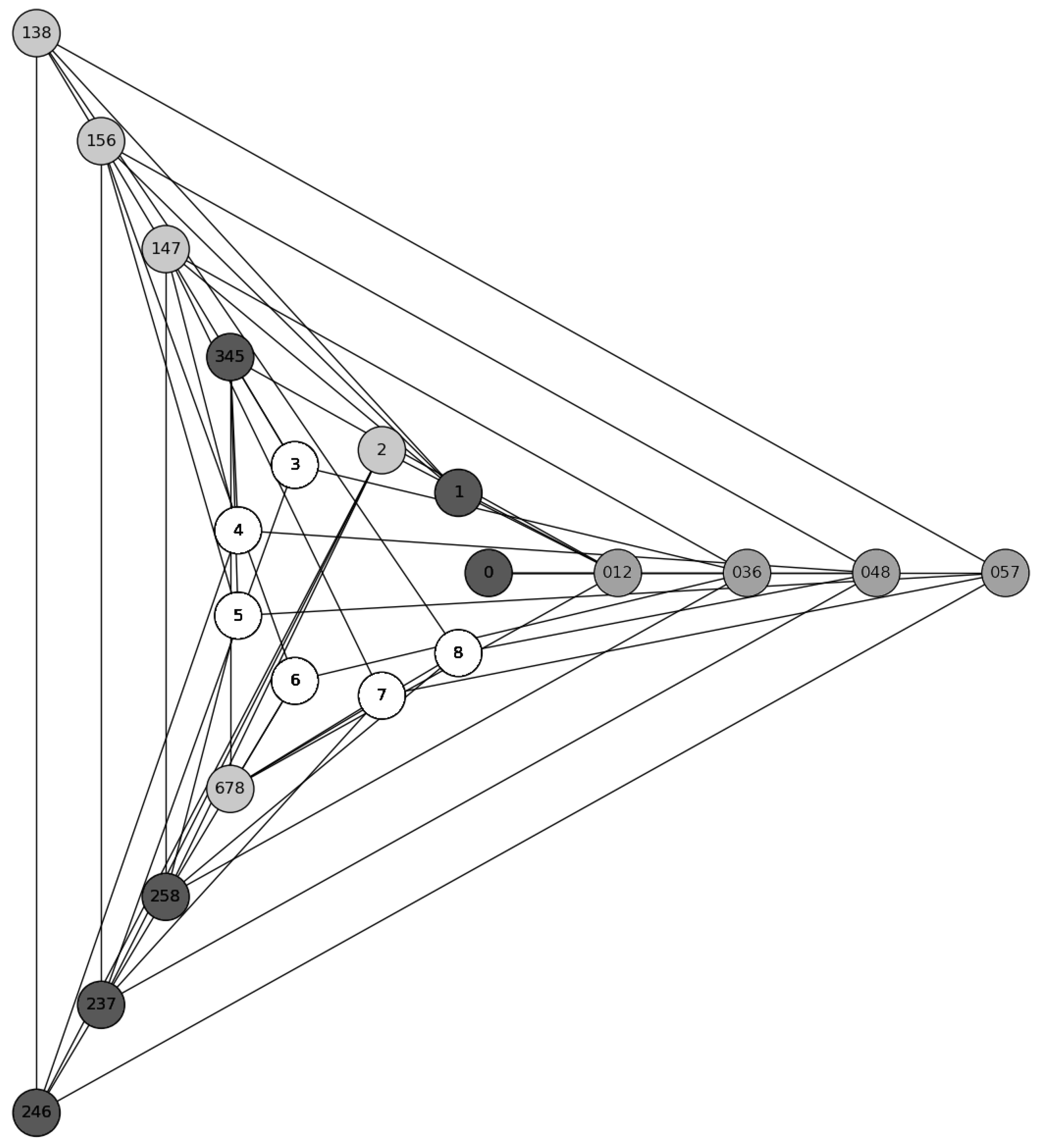
We have seen how we can start with the Hesse SIC and construct four MUB by minimizing the Shannon entropy of the SIC representation, subject to the pure-state constraints. Now, take the nine SIC vectors and twelve MUB vectors, and represent each vector by a vertex of a graph. Connect two vertices with an edge if the corresponding states are orthogonal. The resulting graph has chromatic number 4. That is, one needs at least four different colors of paint in order to color all the vertices in such a way that no two adjacent vertices share the same color. We illustrate this in Figure 1. Because the chromatic number exceeds the dimension of the Hilbert space, this set of 21 vectors meets Cabello’s necessary condition for demonstrating “state-independent contextuality” [27,28].

We now unpack the meaning of this statement.

The issue at stake is whether quantum mechanics could be an approximation to some deeper theory of physics that is classical in character. Could it be that the randomness we find in quantum phenomena might be explained away as due to our ignorance of more fundamental degrees of freedom? A saga of theorems, conceived by Bell, Kochen, Specker and others, argues against this [29]. Quantum theory, they tell us, is incompatible with the idea that quantum uncertainty is a result of our ignorance about “hidden variables” contained within the systems we study (so-called “noncontextual hidden variables”).

It is not a priori obvious exactly which phenomena truly tap into this failure of classicality. Many “quantum” effects can be emulated in models that are essentially classical. The list is remarkably long, in fact, and includes teleportation, key distribution, the no-cloning and no-broadcasting theorems, coherent superpositions turning to incoherent mixtures by becoming entangled with the environment, “quantum discord” and many more [25,30,31,32,33]. However, the Bell-Kochen-Specker results take us out of that regime.

We can think of the Kochen-Specker theorem (and its more modern descendents) in the following way. Suppose that we have some physical system, and we list a series of “questions” that we might ask it. Each question is some physical experiment that yields a quantitative result. For simplicity, we can assume that all these experimental tests are binary, yielding either 0 or 1. Prior to choosing a test and carrying it out, one can have expectations about what will transpire should one choose a particular test and perform it. If we assume that the behavior of the system is governed by some hidden internal degrees of freedom that are independent of the test one might elect to make, then this assumption will constrain the expectations that one might have for the experimental outcomes. The predictions for different experiments will be tied together in a certain way—one which quantum phenomena can violate.

When can a set of questions demonstrate this effect? In quantum theory, we can represent a binary question by a projection operator. A set of projection operators defines an orthogonality graph. A necessary condition for a set of projectors to be able to reveal the failure of the hidden-variable hypothesis is that the chromatic number of their orthogonality graph exceed the dimension of the system’s Hilbert space [27,28]. As explained above, our set of SIC and MUB vectors meets this criterion.

Cabello’s criterion is necessary but not sufficient. However, the Hesse SIC states and the MUB vectors we derived from them are, in fact, sufficient to demonstrate nonclassicality. A Kochen-Specker theorem that demonstrates this explicitly has been worked out [15].

When taken together, the Hesse SIC and its affiliated MUB comprise a set of questions, for which the statistics of the answers mesh together in a way that lies beyond the classical worldview.

5. Conclusions

We began with the issue of compatibility between probability assignments. Extending these considerations from the classical realm to the quantum, we found that the problem of PP-ODOP compatibility for three pure states in three-dimensional Hilbert space leads naturally to SICs and MUB. There are still open questions regarding PP compatibility in higher dimensions [34], and SIC solutions in higher dimensions grow much more complicated than Equation (14). However, the patterns of linear dependencies observed in higher-dimensional SICs [10] suggest that SIC states may have interesting compatibility properties there as well. Likewise, the strategy of finding the pure states whose SIC representations have minimal Shannon entropy yields an intriguing result in dimension 8 [18], and perhaps such states merit attention more generally.