Measurement Uncertainty for Finite Quantum Observables

Abstract

Measurement uncertainty relations are lower bounds on the errors of any approximate joint measurement of two or more quantum observables. The aim of this paper is to provide methods to compute optimal bounds of this type. The basic method is semidefinite programming, which we apply to arbitrary finite collections of projective observables on a finite dimensional Hilbert space. The quantification of errors is based on an arbitrary cost function, which assigns a penalty to getting result x rather than y, for any pair $(x,y)$. This induces a notion of optimal transport cost for a pair of probability distributions, and we include an Appendix with a short summary of optimal transport theory as needed in our context. There are then different ways to form an overall figure of merit from the comparison of distributions. We consider three, which are related to different physical testing scenarios. The most thorough test compares the transport distances between the marginals of a joint measurement and the reference observables for every input state. Less demanding is a test just on the states for which a “true value” is known in the sense that the reference observable yields a definite outcome. Finally, we can measure a deviation as a single expectation value by comparing the two observables on the two parts of a maximally-entangled state. All three error quantities have the property that they vanish if and only if the tested observable is equal to the reference. The theory is illustrated with some characteristic examples.

1. Introduction

Measurement uncertainty relations are quantitative expressions of complementarity. As Bohr often emphasized, the predictions of quantum theory are always relative to some definite experimental arrangement, and these settings often exclude each other. In particular, one has to make a choice of measuring devices, and typically, quantum observables cannot be measured simultaneously. This often used term is actually misleading, because time has nothing to do with it. For a better formulation, recall that quantum experiments are always statistical, so the predictions refer to the frequency with which one will see certain outcomes when the whole experiment is repeated very often. Therefore, the issue is not simultaneous measurement of two observables, but joint measurement in the same shot. That is, a device R is a joint measurement of observable A with outcomes $x\in X$ and observable B with outcomes $y\in Y$, if it produces outcomes of the form $(x,y)$ in such a way that if we ignore outcome y, the statistics of the x outcomes is always (i.e., for every input state) the same as obtained with a measurement of A and symmetrically for ignoring x and comparing to B. It is in this sense that non-commuting projection-valued observables fail to be jointly measurable.

However, this is not the end of the story. One is often interested in approximate joint measurements. One such instance is Heisenberg’s famous γ-ray microscope [1], in which a particle’s position is measured by probing it with light of some wavelength λ, which from the outset sets a scale for the accuracy of this position measurement. Naturally, the particle’s momentum is changed by the Compton scattering, so if we make a momentum measurement on the particles after the interaction, we will find a different distribution from what would have been obtained directly. Note that in this experiment, we get from every particle a position value and a momentum value. Moreover, errors can be quantified by comparing the respective distributions with some ideal reference: the accuracy of the microscope position measurement is judged by the degree of agreement between the distribution obtained and the one an ideal position measurement would give. Similarly, the disturbance of momentum is judged by comparing a directly measured distribution with the one after the interaction. The same is true for the uncontrollable disturbance of momentum. This refers to a scenario where we do not just measure momentum after the interaction, but try to build a device that recovers the momentum in an optimal way, by making an arbitrary measurement on the particle after the interaction, utilizing everything that is known about the microscope, correcting all known systematic errors and even using the outcome of the position measurement. The only requirement is that at the end of the experiment, for each individual shot, some value of momentum must come out. Even then it is impossible to always reproduce the pre-microscope distribution of momentum. The tradeoff between accuracy and disturbance is quantified by a measurement uncertainty relation. Since it simply quantifies the impossibility of a joint exact measurement, it simultaneously gives bounds on how an approximate momentum measurement irretrievably disturbs position. The basic setup is shown in Figure 1.

Figure 1. Basic setup of measurement uncertainty relations. The approximate joint measurement R is shown in the middle, with its array of output probabilities. The marginals $A^{\prime }$ and $B^{\prime }$ of this array are compared to the output probabilities of the reference observables A and B, shown at the top and at the bottom. The uncertainties $\epsilon \left(A^{\prime }\right|A)$ and $\epsilon \left(B^{\prime }\right|B)$ are quantitative measures for the difference between these distributions.

Note that in this description of errors, we did not ever bring in a comparison with some hypothetical “true value”. Indeed, it was noted already by Kennard [2] that such comparisons are problematic in quantum mechanics. Even if one is willing to feign hypotheses about the true value of position, as some hidden variable theorists will, an operational criterion for agreement will always have to be based on statistical criteria, i.e., the comparison of distributions. Another fundamental feature of this view of errors is that it provides a figure of merit for the comparison of two devices, typically some ideal reference observable and an approximate version of it. An “accuracy” ε in this sense is a promise that no matter which input state is chosen, the distributions will not deviate by more than ε. Such a promise does not involve a particular state. This is in contrast to preparation uncertainty relations, which quantify the impossibility to find a state for which the distributions of two given observables (e.g., position and momentum) are both sharp.

Measurement uncertainty relations in the sense described here were first introduced for position and momentum in [3] and were initially largely ignored. A bit earlier, an attempt by Ozawa [4] to quantify error-disturbance tradeoffs with state dependent and somewhat unfortunately chosen [5] quantities had failed, partly for reasons already pointed out in [6]. When experiments confirmed some predictions of the Ozawa approach (including the failure of the error-disturbance tradeoff), a debate ensued [7,8,9,10]. Its unresolved part is whether a meaningful role for Ozawa’s definitions can be found.

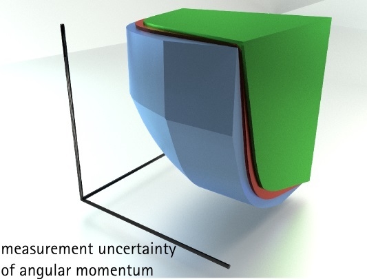
Technically, the computation of measurement uncertainty remained hard, since there were no efficient methods to compute sharp bounds in generic cases. A direct computation along the lines of the definition is not feasible, since it involves three nested optimization problems. The only explicit solutions were for qubits [11,12,13], one case of angular momentum [14] and all cases with phase space symmetry [7,15,16], in which the high symmetry allows the reduction to preparation uncertainty as in [3,9]. The main aim of the current paper is to provide efficient algorithms for sharp measurement uncertainty relations of generic observables, even without any symmetry.

In order to do that, we restrict the setting in some ways, but allow maximal generality in others. We will restrict to finite dimensional systems and reference observables, which are projection valued and non-degenerate. Thus, each of the ideal observables will basically be given by an orthonormal basis in the same d-dimensional Hilbert space. The labels of this basis are the outcomes $x\in X$ of the measurement, where X is a set of d elements. We could choose all $X=\{1,\dots ,d\}$, but it will help to keep track of things using a separate set for each observable. Moreover, this includes the choice $X\subset \mathbb{R}$, the set of eigenvalues of some Hermitian operator. We allow not just two observables, but any finite number $n\ge 2$ of them. This makes some expressions easier to write down, since the sum of an expression involving observable A and an analogous one for observable B becomes an indexed sum. We also allow much generality in the way errors are quantified. In earlier works, we relied on two elements to be chosen for each observable, namely a metric D on the outcome set and an error exponent α, distinguishing, say, absolute ($\alpha =1$), root-mean-square ($\alpha =2$) and maximal ($\alpha =\infty$) deviations. Deviations were then averages of $D{(x,y)}^{\alpha }$. Here, we generalize further to an arbitrary cost function $c:X\times X\to \mathbb{R}$, which we take to be positive and zero exactly on the diagonal (e.g., $c(x,y)=D{(x,y)}^{\alpha }$), but not necessarily symmetric. Again, this generality comes mostly as a simplification of notation. For a reference observable A with outcome set X and an approximate version $A^{\prime }$ with the same outcome set, this defines an error $\epsilon \left(A_{}^{\prime }\right|A_{})$. 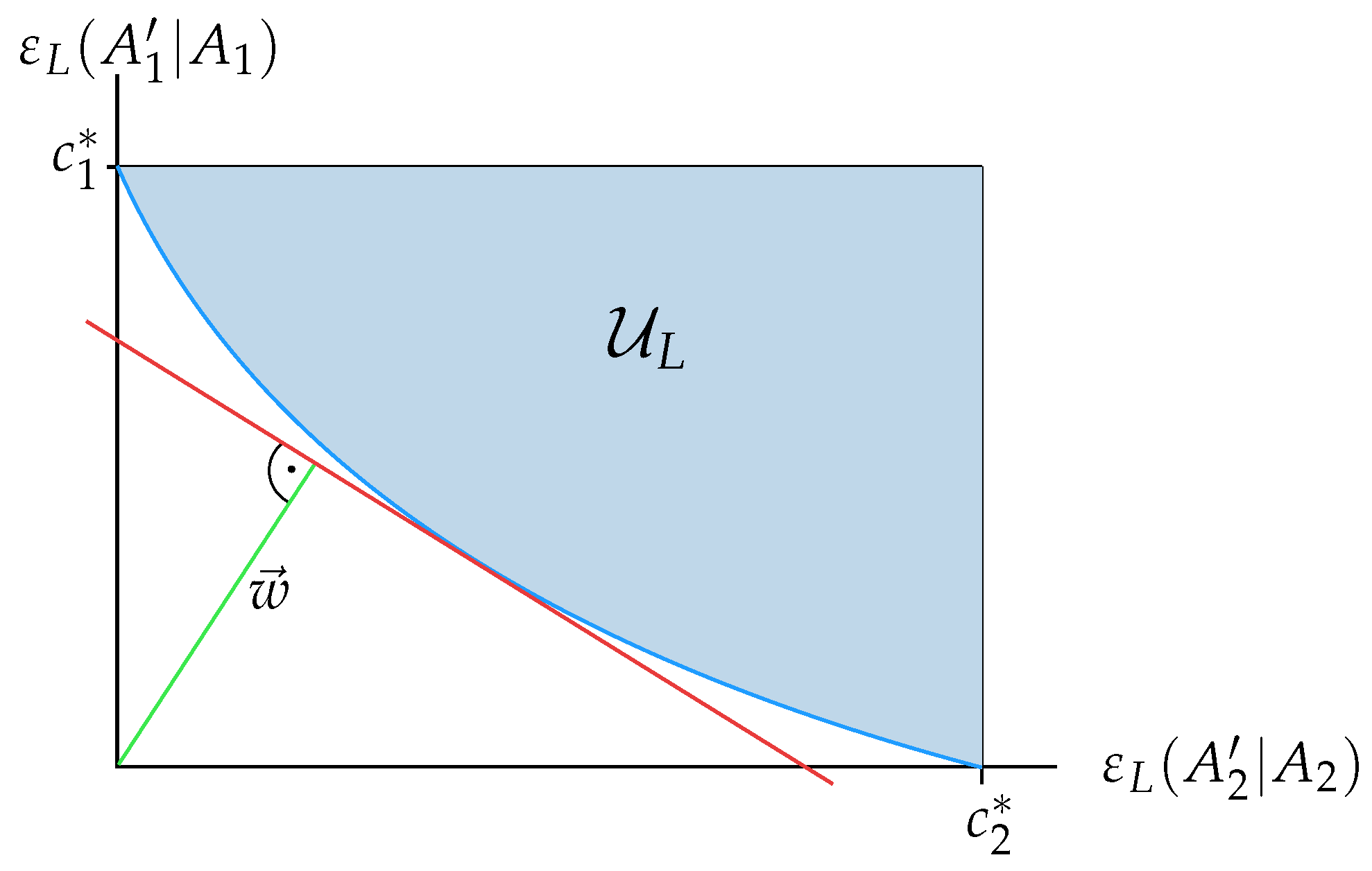Our aim is to provide algorithms for computing the uncertainty diagram associated with such data, of which Figure 2 gives an example. 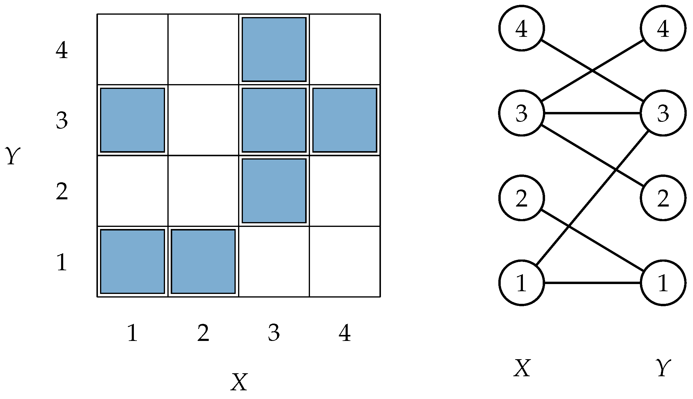The given data for such a diagram are n projection valued observables $A_1,\dots ,A_n$, with outcome sets $X_i$, for each of which we are given also a cost function $c_i:X_i\times X_i\to \mathbb{R}$ for quantifying errors. An approximate joint measurement is then an observable R with outcome set $X_1\times \dots \times X_n$, and hence, with POVMelements $R(x_1,\dots ,x_n)$, where $x_i\in X_i$. By ignoring every output, but one, we get the n marginal observables:

$$A_i^{\prime }\left(x_i\right)=\sum _{x_1,\dots ,x_{i-1},x_{i+1},\dots ,x_n}R(x_1,\dots ,x_n)$$

(1)

and a corresponding tuple:

$$\overrightarrow{\epsilon }\left(R\right)=\left(\epsilon \left(A_1^{\prime }\right|A_1),\dots ,\epsilon \left(A_n^{\prime }\right|A_n)\right)$$

(2)

of errors. The set of such tuples, as R runs over all joint measurements, is the uncertainty region. The surface bounding this set from below describes the uncertainty tradeoffs. For $n=2$, we call it the tradeoff curve. Measurement uncertainty is the phenomenon that, for general reference observables $A_i$, the uncertainty region is bounded away from the origin. In principle, there are many ways to express this mathematically, from a complete characterization of the exact tradeoff curve, which is usually hard to get, to bounds that are simpler to state, but suboptimal. Linear bounds will play a special role in this paper.

Figure 2. Uncertainty regions for three reference observables, namely the angular momentum components $L_1,L_2,L_3$ for spin 1, each with outcome set $X=\{-1,0,+1\}$ and the choice $c(x,y)={(x-y)}^2$ for the cost function. The three regions indicated correspond to the different overall figures of merit ${\epsilon }_M\left(A_{}^{\prime }\right|A_{})\ge {\epsilon }_C\left(A_{}^{\prime }\right|A_{})\ge {\epsilon }_E\left(A_{}^{\prime }\right|A_{})$ described in Section 2.

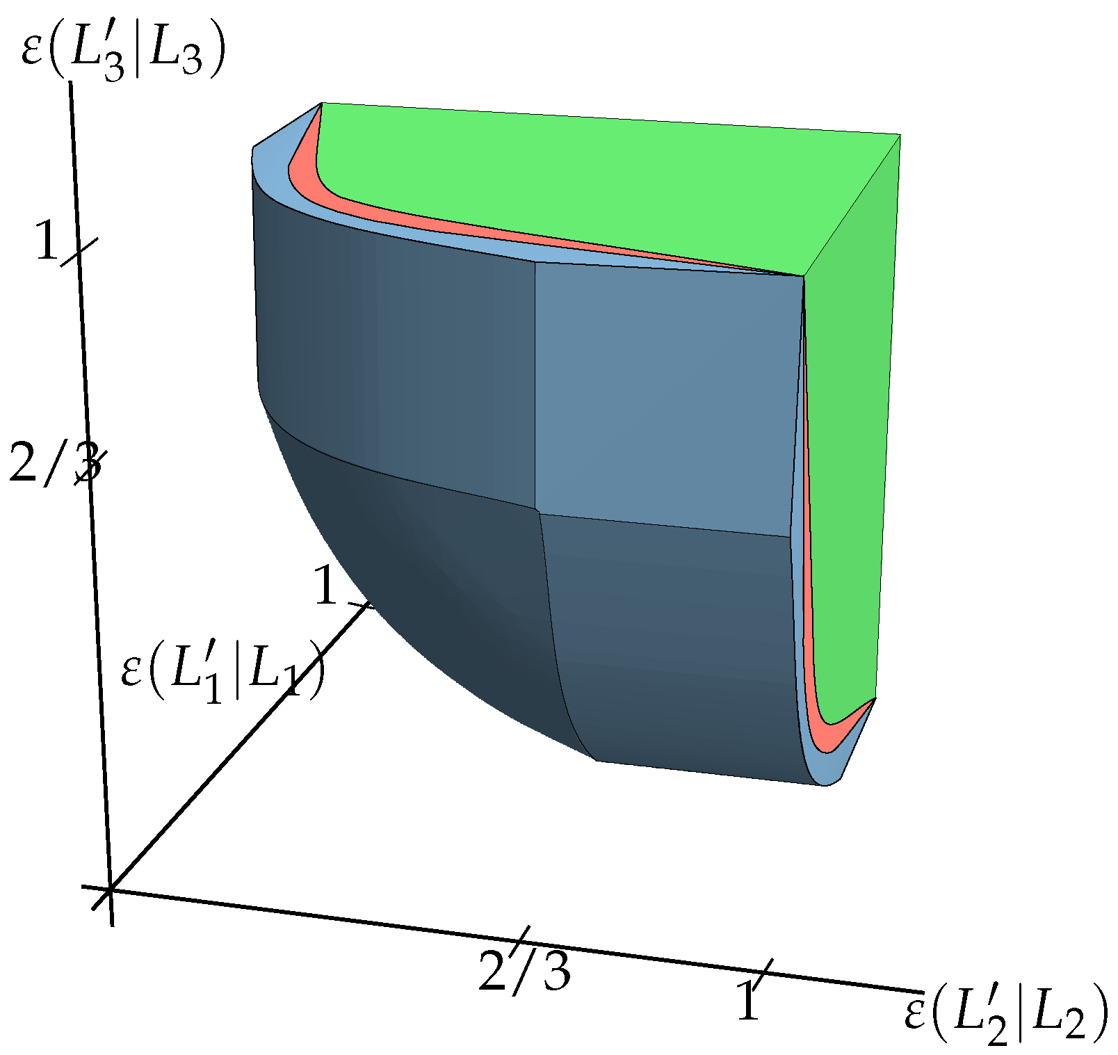
We will consider three ways to build a single error quantity out of the comparison of distributions, denoted by ${\epsilon }_M\left(A_{}^{\prime }\right|A_{})$, ${\epsilon }_C\left(A_{}^{\prime }\right|A_{})$ and ${\epsilon }_E\left(A_{}^{\prime }\right|A_{})$. These will be defined in Section 2. For every choice of observables and cost functions, each will give an uncertainty region, denoted by ${\mathcal{U}}_M$, ${\mathcal{U}}_C$ and ${\mathcal{U}}_E$, respectively. Since they are all based on the same cost function c, they are directly comparable (see Figure 2). We show in Section 3 that the three regions are convex and hence characterized completely by linear bounds. In Section 4, we show how to calculate the optimal linear lower bounds by semidefinite programs. Finally, an Appendix collects the basic information on the beautiful theory of optimal transport, which is needed in Section 2.1 and Section 4.1.

2. Deviation Measures for Observables

Here, we define the measures we use to quantify how well an observable $A^{\prime }$ approximates a desired observable A. In this section, we do not use the marginal condition Equation (1), so $A^{\prime }$ is an arbitrary observable with the same outcome set X as A, i.e., we drop all indices i identifying the different observables. Our error quantities are operational in the sense that each is motivated by an experimental setup, which will in particular provide a natural way to measure them. All error definitions are based on the same cost function $c:X\times X\to \mathbb{R}$, where $c(x,y)$ is the “cost” of getting a result $x\in X$, when $y\in X$ would have been correct. The only assumptions are that $c(x,y)\ge 0$ with $c(x,y)=0$ iff $x=y$.

As described above, we consider a quantum system with Hilbert space ${\mathbb{C}}^d$. As a reference observable A, we allow any complete von Neumann measurement on this system, that is any observable whose set X of possible measurement outcomes has size $\left|X\right|=d$ and whose POVM elements $A\left(y\right)\in \mathcal{B}\left({\mathbb{C}}^d\right)$ ($y\in X$) are mutually orthogonal projectors of rank 1; we can then also write $A\left(y\right)=|{\varphi }_y⟩⟨{\varphi }_y|$ with an orthonormal basis $\left\{{\varphi }_y\right\}$ of ${\mathbb{C}}^d$. For the approximating observable $A^{\prime }$, the POVM elements $A^{\prime }\left(x\right)$ (with $x\in X$) are arbitrary with $A^{\prime }\left(x\right)\ge 0$ and ${\sum }_{x\in X}A\left(x\right)=\mathrm{𝟙}$.

The comparison will be based on a comparison of output distributions, for which we use the following notations: given a quantum state ρ on this system, i.e., an operator with $\rho \ge 0$ and $tr\rho =1$, and an observable, such as A, we will denote the outcome distribution by $\rho A$, so $\left(\rho A\right)\left(y\right):=tr\left(\rho A_y\right)$. This is a probability distribution on the outcome set X and can be determined physically as the empirical outcome distribution after many experiments.

For comparing just two probability distributions $p:X\to {\mathbb{R}}_{+}$ and $q:X\to {\mathbb{R}}_{+}$, a canonical choice is the “minimum transport cost”:

$$\check{c}(p,q):=\underset{\gamma }{inf}\left\{\sum _{xy}c(x,y)\gamma (x,y)|\gamma \mathrm{couples}p\mathrm{to}q\right\}$$

(3)

where the infimum runs over the set of all couplings or “transport plans” $\gamma :X\times X\to {\mathbb{R}}_{+}$ of p to q, i.e., the set of all probability distributions γ satisfying the marginal conditions ${\sum }_y\gamma (x,y)=p\left(x\right)$ and ${\sum }_x\gamma (x,y)=q\left(y\right)$. The motivations for this notion and the methods to compute it efficiently are described in the Appendix. Since X is finite, the infimum is over a compact set, so it is always attained. Moreover, since we assumed $c\ge 0$ and $c(x,y)=0\iff x=y$, we also have $\check{c}(p,q)\ge 0$ with equality iff $p=q$. If one of the distributions, say q, is concentrated on a point $\tilde{y}$, only one coupling exists, namely $\gamma (x,y)=p\left(x\right){\delta }_{y\tilde{y}}$. In this case, we abbreviate $\check{c}(p,q)=\check{c}(p,\tilde{y})$, and get:

$$\check{c}(p,\tilde{y})=\sum _{x}p\left(x\right)c(x,\tilde{y})$$

(4)

i.e., the average cost of moving all of the points x distributed according to p to $\tilde{y}$.

2.1. Maximal Measurement Error ${\epsilon }_M\left(A_{}^{\prime }\right|A_{})$

The worst case error over all input states is:

$${\epsilon }_M\left(A_{}^{\prime }\right|A_{}):=\underset{\rho }{sup}\left\{\check{c}(\rho A^{\prime },\rho A)| \rho \text{quantum}\text{state}\text{on}{\mathbb{C}}^d\right\}$$

(5)

which we call the maximal error. Note that, like the cost function c and the transport costs $\check{c}$, the measure ${\epsilon }_M\left(A_{}^{\prime }\right|A_{})$ need not be symmetric in its arguments, which is sensible, as the reference and approximating observables have distinct roles. Similar definitions for the deviation of an approximating measurement from an ideal one have been made, for specific cost functions, in [7,9] and [14] before.

The definition Equation (5) makes sense even if the reference observable A is not a von Neumann measurement. Instead, the only requirement is that A and $A^{\prime }$ be general observables with the same (finite) outcome set X, not necessarily of size d. All of our results below that involve only the maximal measurement error immediately generalize to this case, as well.

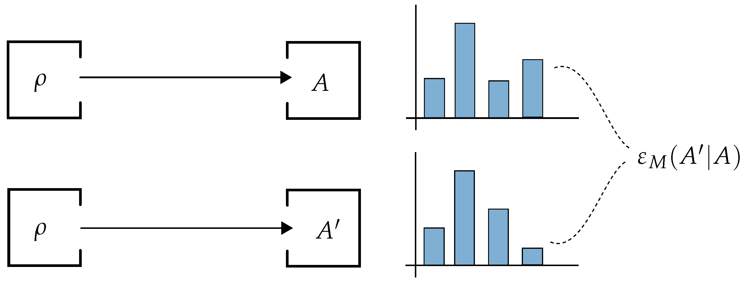
One can see that it is expensive to determine the quantity ${\epsilon }_M\left(A_{}^{\prime }\right|A_{})$ experimentally according to the definition: one would have to measure and compare (see Figure 3) the outcome statistics $\rho A^{\prime }$ and $\rho A$ for all possible input states ρ, which form a continuous set. The following definition of observable deviation alleviates this burden.

Figure 3. For the maximal measurement error ${\epsilon }_M\left(A_{}^{\prime }\right|A_{})$ the transport distance of output distributions is maximized over all input states ρ.

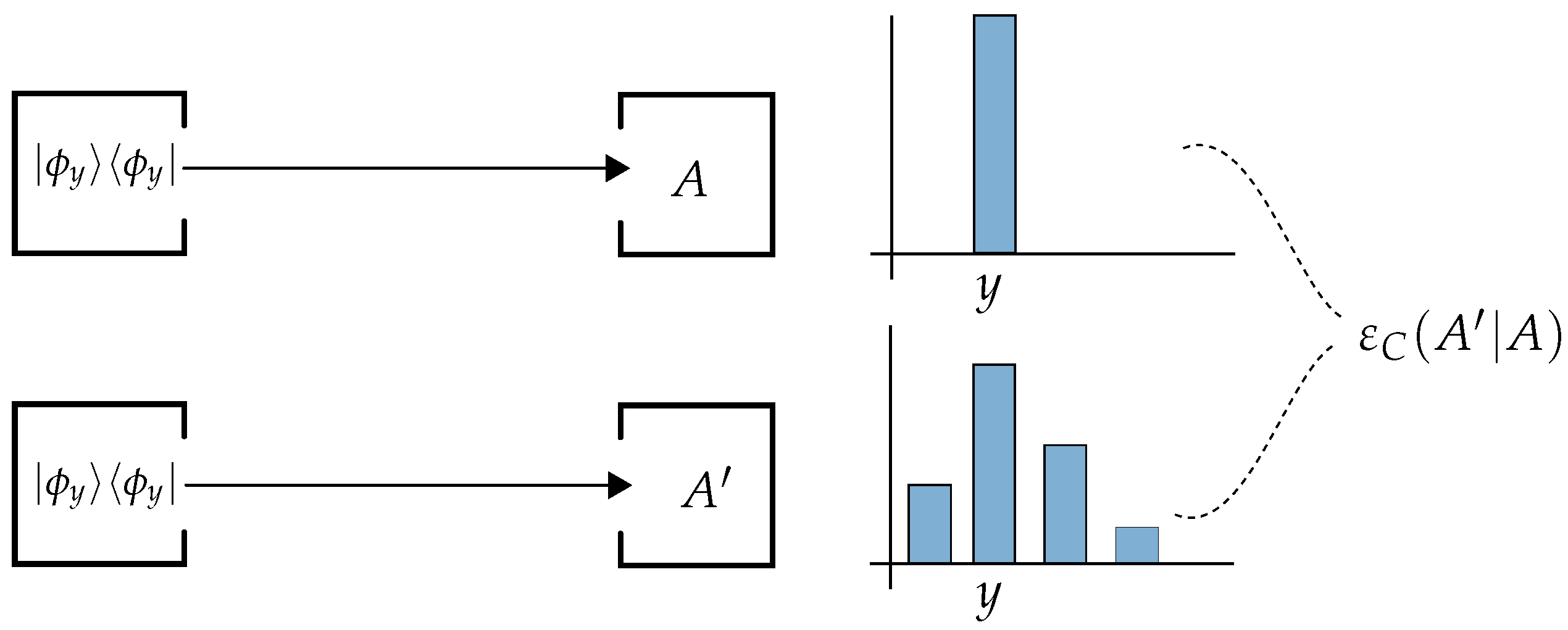
2.2. Calibration Error ${\epsilon }_C\left(A_{}^{\prime }\right|A_{})$

Calibration (see Figure 4) is a process by which one tests a measuring device on inputs (or measured objects) for which the “true value” is known. Even in quantum mechanics, we can set this up by demanding that the measurement of the reference observable on the input state gives a sharp value y. In a general scenario with continuous outcomes, this can only be asked with a finite error δ, which goes to zero at the end [7], but in the present finite scenario, we can just demand $\left(\rho A\right)\left(y\right)=1$. Since, for every outcome y of a von Neumann measurement, there is only one state with this property (namely $\rho =|{\varphi }_y⟩⟨{\varphi }_y|$), we can simplify even further, and define the calibration error by:

$${\epsilon }_C\left(A_{}^{\prime }\right|A_{}):=\underset{y,\rho }{sup}\left\{\check{c}(\rho A^{\prime },y)\right|tr\left(\rho A\left(y\right)\right)=1\}=\underset{y}{max}\sum _x⟨{\varphi }_y|A^{\prime }\left(x\right)|{\varphi }_y⟩c(x,y)$$

(6)

Figure 4. For the calibration error ${\epsilon }_C\left(A_{}^{\prime }\right|A_{})$, the input state is constrained to the eigenstates of A, say with sharp A-value y, and the cost of moving the $A^{\prime }$-distribution to y is maximized over y.

Note that the calibration idea only makes sense when there are sufficiently many states for which the reference observable has deterministic outcomes, i.e., for projective observables A.

A closely related quantity has recently been proposed by Appleby [10]. It is formulated for real valued quantities with cost function $c(x,y)={(x-y)}^2$ and has the virtue that it can be expressed entirely in terms of first and second moments of the probability distributions involved. Therefore, for any ρ, let m and v be the mean and variance of $\rho A$ and $v^{\prime }$ the mean quadratic deviation of $\rho A^{\prime }$ from m. Then, Appleby defines:

$${\epsilon }_D\left(A_{}^{\prime }\right|A_{})=\underset{\rho }{sup}{(\sqrt{v^{\prime }}-\sqrt{v})}^2$$

(7)

Here, we added the square to make Appleby’s quantity comparable to our variance-like (rather than standard deviation-like) quantities and chose the letter D, because Appleby calls this the D-error. Since in the supremum, we have also the states for which A has a sharp distribution (i.e., $v=0$), we clearly have ${\epsilon }_D\left(A_{}^{\prime }\right|A_{})\ge {\epsilon }_C\left(A_{}^{\prime }\right|A_{})$. On the other hand, let $\mathrm{\Phi }\left(x\right)=t{(x-m)}^2$ and $\mathrm{\Psi }\left(y\right)=t/(1-t){(y-m)}^2$. Then, one easily checks that $\mathrm{\Phi }\left(x\right)-\mathrm{\Psi }\left(y\right)\le {(x-y)}^2$, so $(\mathrm{\Phi },\mathrm{\Psi })$ is a pricing scheme in the sense defined in the Appendix. Therefore:

$$\check{c}(\rho A^{\prime },\rho A)\ge \sum _x\left(\rho A^{\prime }\right)\left(x\right)\mathrm{\Phi }\left(x\right)-\sum _y\left(\rho A\right)\left(y\right)\mathrm{\Psi }\left(y\right)=t{v}^{\prime }-\frac{t}{1-t}v$$

(8)

Maximizing this expression over t gives exactly Equation (7). Therefore,

$${\epsilon }_C\left(A_{}^{\prime }\right|A_{})\le {\epsilon }_D\left(A_{}^{\prime }\right|A_{})\le {\epsilon }_M\left(A_{}^{\prime }\right|A_{}).$$

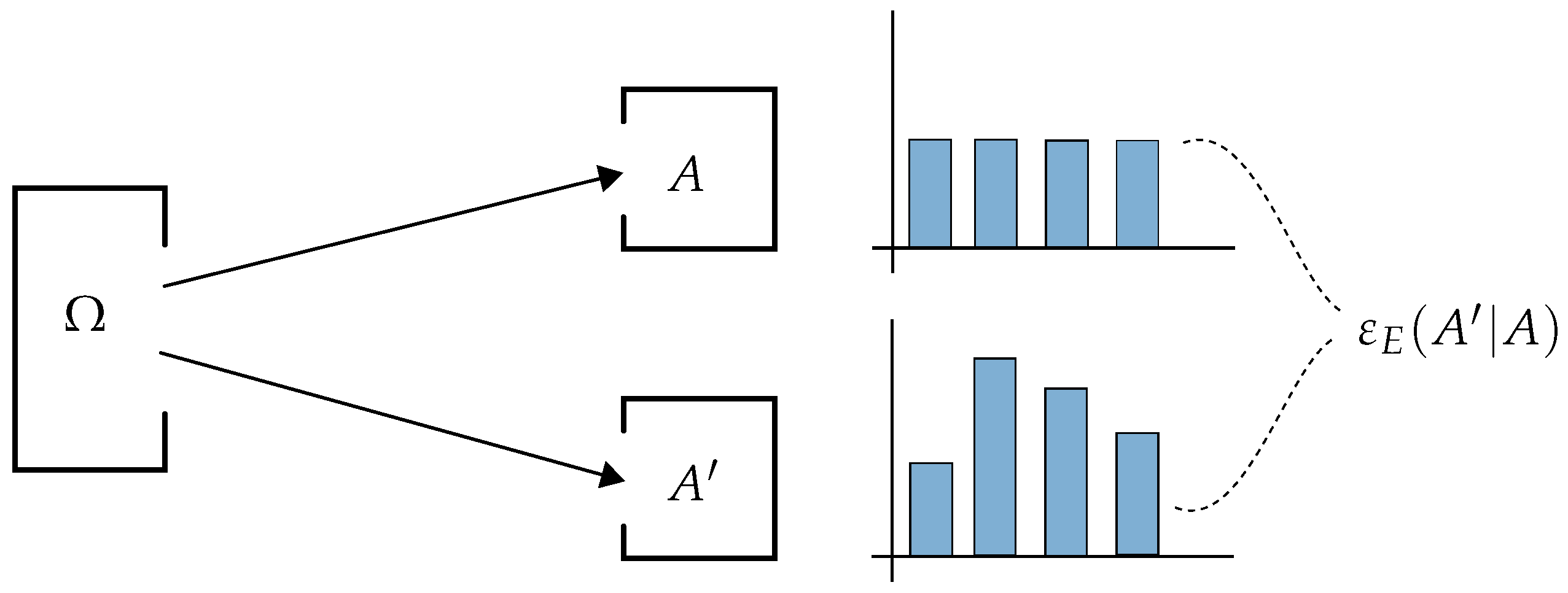
2.3. Entangled Reference Error ${\epsilon }_E\left(A_{}^{\prime }\right|A_{})$

In quantum information theory, a standard way of providing a reference state for later comparison is by applying a channel or observable to one half of a maximally-entangled system. Two observables would be compared by measuring them (or suitable modifications) on the two parts of a maximally-entangled system (see Figure 5). Let us denote the entangled vector by $\mathrm{\Omega }=d^{-1/2}{\sum }_k|kk⟩$. Since later, we will look at several distinct reference observables, the basis kets $|k⟩$ in this expression have no special relation to A or its eigenbasis ${\varphi }_y$. We denote by $X^{\mathsf{T}}$ the transpose of an operator X in the $|k⟩$ basis, and by $A^{\mathsf{T}}$ the observable with POVM elements $A{\left(y\right)}^{\mathsf{T}}=|\overline{{\varphi }_y}⟩⟨\overline{{\varphi }_y}|$, where $\overline{{\varphi }_y}$ is the complex conjugate of ${\varphi }_y$ in $|k⟩$-basis. These transposes are needed due to the well-known relation $(X\otimes \mathrm{𝟙})\mathrm{\Omega }=(\mathrm{𝟙}\otimes X^{\mathsf{T}})\mathrm{\Omega }$. We now consider an experiment, in which $A^{\prime }$ is measured on the first part and $A^{\mathsf{T}}$ on the second part of the entangled system, so we get the outcome pair $(x,y)$ with probability:

$$p(x,y)=⟨\mathrm{\Omega }|A^{\prime }\left(x\right)\otimes A{\left(y\right)}^{\mathsf{T}}|\mathrm{\Omega }⟩=⟨\mathrm{\Omega }|A^{\prime }\left(x\right)A\left(y\right)\otimes \mathrm{𝟙}|\mathrm{\Omega }⟩=\frac{1}{d}tr\left(A^{\prime }\left(x\right)A\left(y\right)\right)$$

(9)

Figure 5. The entangled reference error ${\epsilon }_E\left(A_{}^{\prime }\right|A_{})$ is a single expectation value, namely of the cost $c(x,y)$, where y is the output of $A^{\mathsf{T}}$ and x the output of $A^{\prime }$. Like the other error quantities, this expectation vanishes iff $A^{\prime }=A$.

As A is a complete von Neumann measurement, this probability distribution is concentrated on the diagonal ($x=y$) iff $A^{\prime }=A$, i.e., there are no errors of $A^{\prime }$ relative to A. Averaging with the error costs, we get a quantity we call the entangled reference error:

$${\epsilon }_E\left(A_{}^{\prime }\right|A_{}):=\sum _{xy}\frac{1}{d}tr\left(A^{\prime }\left(x\right)A\left(y\right)\right)c(x,y)$$

(10)

Note that this quantity is measured as a single expectation value in the experiment with source Ω. Moreover, when we later want to measure different such deviations for the various marginals, the source and the tested joint measurement device can be kept fixed, and only the various reference observables $A_i^{\mathsf{T}}$ acting on the second part need to be adapted suitably.

2.4. Summary and Comparison

The quantities ${\epsilon }_M\left(A_{}^{\prime }\right|A_{})$, ${\epsilon }_C\left(A_{}^{\prime }\right|A_{})$ and ${\epsilon }_E\left(A_{}^{\prime }\right|A_{})$ constitute three different ways to quantify the deviation of an observable $A^{\prime }$ from a projective reference observable A. Nevertheless, they are all based on the same distance-like measure, the cost function c on the outcome set X. Therefore, it makes sense to compare them quantitatively. Indeed, they are ordered as follows:

$${\epsilon }_M\left(A_{}^{\prime }\right|A_{})\ge {\epsilon }_C\left(A_{}^{\prime }\right|A_{})\ge {\epsilon }_E\left(A_{}^{\prime }\right|A_{})$$

(11)

Here, the first inequality follows by restricting the supremum Equation (5) to states that are sharp for A and the second by noting that the Equation (6) is the maximum of a function of y, of which Equation (10) is the average.

Moreover, as we argued before in Equation (10), ${\epsilon }_E\left(A_{}^{\prime }\right|A_{})=0$ if and only if $A=A^{\prime }$, which is hence equivalent also to ${\epsilon }_M\left(A_{}^{\prime }\right|A_{})=0$ and ${\epsilon }_C\left(A_{}^{\prime }\right|A_{})=0$.

3. Convexity of Uncertainty Diagrams

For two observables $B_1$ and $B_2$ with the same outcome set, we can easily realize their mixture or convex combination $B=t{B}_1+(1-t)B_2$ by flipping a coin with probability t for heads in each instance and then apply $B_1$ when heads is up and $B_2$ otherwise. In terms of POVM elements, this reads $B\left(x\right)=t{B}_1\left(x\right)+(1-t)B_2\left(x\right)$. We show first that this mixing operation does not increase the error quantities from Section 2.

Lemma 1. 

For $L\in \{M,D,C,E\}$ the error quantity ${\epsilon }_L\left(B\right|A)$, is a convex function of B, i.e., for $B=t{B}_1+(1-t)B_2$ and $t\in [0,1]$:

$$\begin{array}{cc}\hfill {\epsilon }_L\left(B\right|A)& \le t{\epsilon }_L\left(B_1\right|A)+(1-t){\epsilon }_L\left(B_1\right|A)\hfill \end{array}$$

(12)

Proof. 

The basic fact used here is that the pointwise supremum of affine functions (i.e., those for which equality holds in the definition of a convex function) is convex. This is geometrically obvious and easily verified from the definitions. Hence, we only have to check that each of the error quantities is indeed represented as a supremum of functions, which are affine in the observable B.

For $L=E$, we even get an affine function, because Equation (10) is linear in $A^{\prime }$. For $L=C$, Equation (6) has the required form. For $L=M$, Equation (5) is a supremum, but the function $\check{c}$ is defined as an infimum. However, we can use the duality theory described in the Appendix to write it instead as a supremum over pricing schemes, of an expression that is just the expectation of $\mathrm{\Phi }\left(x\right)$ plus a constant and, therefore, an affine function. Finally, for Appleby’s case Equation (7), we get the same supremum, but over the subset of pricing schemes (the quadratic ones).  ☐

The convexity of the error quantities distinguishes measurement from preparation uncertainty. Indeed, the variances appearing in preparation uncertainty relations are typically concave functions, because they arise from minimizing the expectation of ${(x-m)}^2$ over m. Consequently, the preparation uncertainty regions may have gaps and non-trivial behavior on the side of large variances. The following proposition will show that measurement uncertainty regions are better behaved.

For every cost function c on a set X, we can define a “radius” ${\overline{c}}^{*}$, the largest transportation cost from the uniform distribution (the “center” of the set of probability distributions) and a “diameter” $c^{*}$, the largest transportation cost between any two distributions:

$${\overline{c}}^{*}=\underset{y}{max}\sum _{x}c(x,y)/d{c}^{*}=ma{x}_{xy}c(x,y)$$

(13)

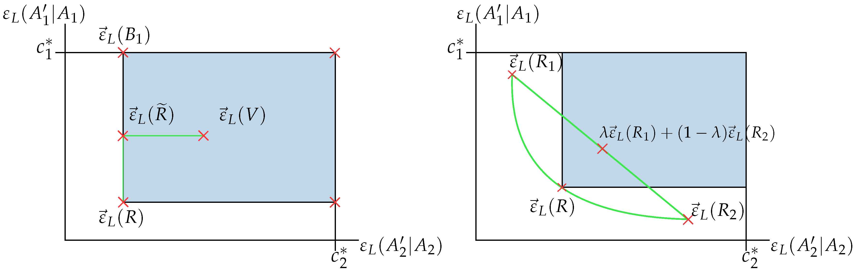
Proposition 2. 

Let n observables $A_i$ and cost functions $c_i$ be given, and define $c_i^M=c_i^C=c_i^{*}$ and $c_i^E={\overline{c_i}}^{*}$. Then, for $L=\{M,C,E\}$, the uncertainty regions ${\mathcal{U}}_L$ is a convex set and has the following (monotonicity) property: when $\overrightarrow{x}=(x_1,\dots ,x_n)\in {\mathcal{U}}_L$ and $\overrightarrow{y}=(y_i,\dots ,y_n)\in {\mathbb{R}}^n$ are such that $x_i\le y_i\le c_i^L$, then $\overrightarrow{y}\in {\mathcal{U}}_L$.

Proof. 

Let us first clarify how to make the worst possible measurement B, according to the various error criteria, for which we go back to the setting of Section 2, with just one observable A and cost function c. In all cases, the worst measurement is one with constant and deterministic output, i.e., $B\left(x\right)={\delta }_{x^{*},x}\mathrm{𝟙}$. For $L=C$ and $L=M$, such a measurement will have ${\epsilon }_L\left(B\right|A)={max}_{y}c(x^{*},y)$, and we can choose $x^{*}$ to make this equal to $c^{*}=c^L$. For $L=E$, we get instead the average, which is maximized by ${\overline{c}}^{*}$.

We can now make a given joint measurement R worse by replacing it partly by a bad one, say for the first observable $A_1$. That is, we set, for $\lambda \in [0,1]$,

$$\tilde{R}(x_1,x_2,\dots ,x_n)=\lambda B_1\left(x_1\right)\sum _{y_1}R(y_1,x_2,\dots ,x_n)+(1-\lambda )R(x_1,x_2,\dots ,x_n)$$

(14)

Then, all marginals ${\tilde{A}}_i^{\prime }$ for $i\ne 1$ are unchanged, but ${\tilde{A}}_1^{\prime }\left(x_1\right)=\lambda B_1\left(x_1\right)+(1-\lambda )A^{\prime }\left(x_1\right)$. Now, as λ changes from zero to one, the point in the uncertainty diagram will move continuously in the first coordinate direction from $\overrightarrow{x}$ to the point in which the first coordinate is replaced by its maximum value (see Figure 6 (left)). Obviously, the same holds for every other coordinate direction, which proves the monotonicity statement of the proposition.

Figure 6. The blue shaded region corresponds to the monotonicity statement for ${\overrightarrow{\epsilon }}_L\left(R\right)$. (Left) $\tilde{R}$ is a mixture of R and $B_1$. We can also get an observable V by mixing the second marginal of $\tilde{R}$ with $B_2$ and, thus, reach every point in the blue shaded region. (Right) ${\overrightarrow{\epsilon }}_L\left(R\right)$ is componentwise convex. Therefore, the mixture of the points ${\overrightarrow{\epsilon }}_L\left(R\right)$ and ${\overrightarrow{\epsilon }}_L\left(R\right)$ is always in the monotonicity region corresponding to ${\overrightarrow{\epsilon }}_L\left(R\right)$.

Let $R_1$ and $R_2$ be two observables, and let $R=\lambda R_1+(1-\lambda )R_2$ be their mixture. For proving the convexity of ${\mathcal{U}}_L$, we will have to show that every point on the line between ${\overrightarrow{\epsilon }}_L\left(R_1\right)$ and ${\overrightarrow{\epsilon }}_L\left(R_2\right)$ can be attained by a tuple of errors corresponding to some allowed observable (see Figure 6 (right)). Now, lemma 1 tells us that every component of ${\overrightarrow{\epsilon }}_L\left(R\right)$ is convex, which implies that ${\overrightarrow{\epsilon }}_L\left(R\right)\le \lambda {\overrightarrow{\epsilon }}_L\left(R_1\right)+(1-\lambda ){\overrightarrow{\epsilon }}_L\left(R_2\right)$. However, by monotonicity, this also means that $\lambda {\overrightarrow{\epsilon }}_L\left(R_1\right)+(1-\lambda )\overrightarrow{\epsilon }\left(R_2\right)$ is in ${\mathcal{U}}_L$ again, which shows the convexity of ${\mathcal{U}}_L$. ☐

Example: Phase Space Pairs

As is plainly visible from Figure 2, the three error criteria considered here usually give different results. However, under suitable circumstances, they all coincide. This is the case for conjugate pairs related by Fourier transform [15]. The techniques needed to show this are the same as for the standard position/momentum case [9,17] and, in addition, imply that the region for preparation uncertainty is also the same.

In the finite case, there is not much to choose: we have to start from a finite abelian group, which we think of as position space, and its dual group, which is then the analogue of momentum space. The unitary connecting the two observables is the finite Fourier associated with the group. The cost function needs to be translation invariant, i.e., $c(x,y)=c(x-y)$. Then, by an averaging argument, we find for all error measures that a covariant phase space observable minimizes measurement uncertainty (all three versions). The marginals of such an observable can be simulated by first doing the corresponding reference measurement and then adding some random noise. This implies [14] that ${\epsilon }_M\left(A_{}^{\prime }\right|A_{})={\epsilon }_C\left(A_{}^{\prime }\right|A_{})$. However, we know more about this noise: it is independent of the input state, so that the average and the maximum of the noise (as a function of the input) coincide, i.e., ${\epsilon }_C\left(A_{}^{\prime }\right|A_{})={\epsilon }_E\left(A_{}^{\prime }\right|A_{})$. Finally, we know that the noise of the position marginal is distributed according to the position distribution of a certain quantum state, which is, up to normalization and a unitary parity inversion, the POVM element of the covariant phase space observable at the origin. The same holds for the momentum noise. However, then the two noise quantities are exactly related like the position and momentum distributions of a state, and the tradeoff curve for that problem is exactly preparation uncertainty, with variance criteria based on the same cost function.

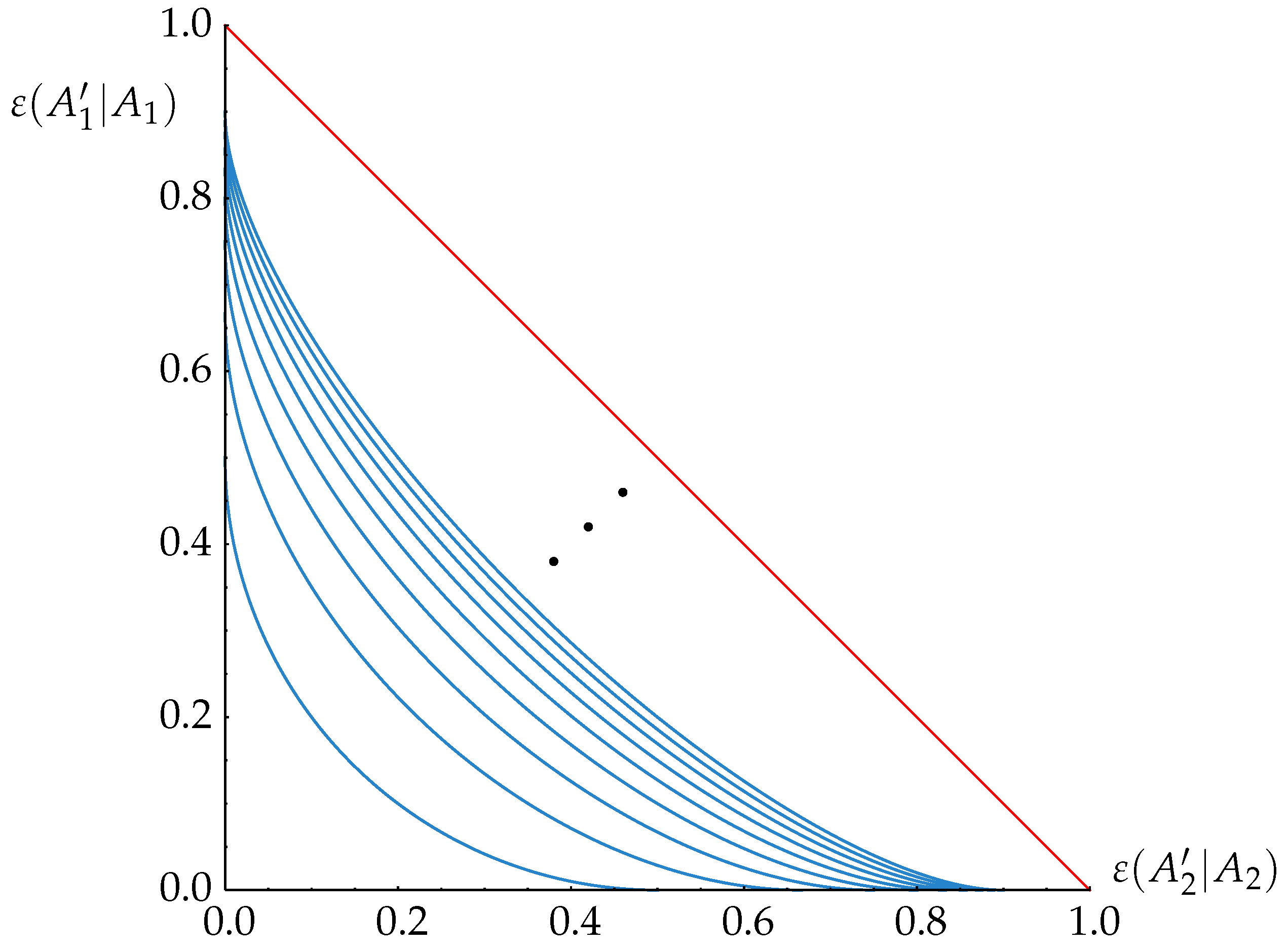
If we choose the discrete metric for c, the uncertainty region depends only on the number d of elements in the group we started from [15]. The largest ε for all quantities is the distance from a maximally-mixed state to any pure state, which is $\Delta =(1-1/d)$. The exact tradeoff curve is then an ellipse, touching the axes at the points $(0,\Delta )$ and $(\Delta ,0)$. The resulting family of curves, parameterized by d, is shown in Figure 7. In general, however, the tradeoff curve requires the solution of a non-trivial family of ground state problems and cannot be given in closed form. For bit strings of length n and the cost, some convex function of Hamming distance there is an expression for large n [15].

Figure 7. The uncertainty tradeoff curves for discrete position/momentum pairs, with a discrete metric. In this case, all uncertainty regions, also the one for preparation uncertainty, coincide. The parameter of the above tradeoff curves is the order $d=2,3,\dots ,10,\cdots ,\infty$ of the underlying abelian group.

4. Computing Uncertainty Regions via Semidefinite Programming

We show here how the uncertainty regions, and therefore, optimal uncertainty relations, corresponding to each of the three error measures can actually be computed, for any given set of projective observables $A_1,\dots ,A_n$ and cost functions $c_1,\dots ,c_n$. Our algorithms will come in the form of semidefinite programs (SDPs) [18,19], facilitating efficient numerical computation of the uncertainty regions via the many existing program packages to solve SDPs. Moreover, the accuracy of such numerical results can be rigorously certified via the duality theory of SDPs. To obtain the illustrations in this paper, we used the CVX package [20,21] under MATLAB.

As all of our uncertainty regions ${\mathcal{U}}_L\subset {\mathbb{R}}^n$ (for $L=M,C,E$) are convex and closed (Section 3), they are completely characterized by their supporting hyperplanes (for a reference to convex geometry, see [22]). Due to the monotonicity property stated in Proposition 2, some of these hyperplanes just cut off the set parallel along the planes $x_i=c_i^L$. The only hyperplanes of interest are those with nonnegative normal vectors $\overrightarrow{w}=(w_1,\dots ,w_n)\in {\mathbb{R}}_{+}^n$ (see Figure 8). Each hyperplane is completely specified by its “offset” $b_L\left(\overrightarrow{w}\right)$ away from the origin, and this function determines ${\mathcal{U}}_L$:

$$\begin{array}{ccc}\hfill b_L\left(\overrightarrow{w}\right)& :=& inf\left\{\overrightarrow{w}·\overrightarrow{\epsilon }|\overrightarrow{\epsilon }\in {\mathcal{U}}_L\right\}\hfill \end{array}$$

(15)

$$\begin{array}{ccc}\hfill {\mathcal{U}}_L& =& \left\{\overrightarrow{\epsilon }\in {\mathbb{R}}^n|\forall \overrightarrow{w}\in {\mathbb{R}}_{+}^n\overrightarrow{w}·\overrightarrow{\epsilon }\ge b_L\left(\overrightarrow{w}\right)\right\}\hfill \end{array}$$

(16)

Figure 8. The lower bound of the uncertainty region ${\mathcal{U}}_L$ can be described by its supporting hyperplanes (red line) with a normal vector $\overrightarrow{w}\in {\mathbb{R}}_{+}^n$.

In fact, due to homogeneity $b_L\left(t\overrightarrow{w}\right)=t{b}_L\left(\overrightarrow{w}\right)$, we can restrict everywhere to the subset of vectors $\overrightarrow{w}\in {\mathbb{R}}_{+}^n$ that, for example, satisfy ${\sum }_i{w}_i=1$, suggesting an interpretation of the $w_i$ as weights of the different uncertainties ${\epsilon }_i$. Our algorithms will, besides evaluating $b_L\left(\overrightarrow{w}\right)$, also allow one to compute a (approximate) minimizer $\overrightarrow{\epsilon }$, so that one can plot the boundary of the uncertainty region ${\mathcal{U}}_L$ by sampling over $\overrightarrow{w}$, which is how the figures in this paper were obtained.

Let us further note that knowledge of $b_L\left(\overrightarrow{w}\right)$ for some $\overrightarrow{w}\in {\mathbb{R}}_{+}^n$ immediately yields a quantitative uncertainty relation: every error tuple $\overrightarrow{\epsilon }\in {\mathcal{U}}_L$ attainable via a joint measurement is constrained by the affine inequality $\overrightarrow{w}·\overrightarrow{\epsilon }\ge b_L\left(\overrightarrow{w}\right)$, meaning that some weighted average of the attainable error quantities ${\epsilon }_i$ cannot become too small. When $b_L\left(\overrightarrow{w}\right)>0$ is strictly positive, this excludes in particular the zero error point $\overrightarrow{\epsilon }=\overrightarrow{0}$. The obtained uncertainty relations are optimal in the sense that there exists $\overrightarrow{\epsilon }\in {\mathcal{U}}_L$, which attains strict equality $\overrightarrow{w}·\overrightarrow{\epsilon }=b_L\left(\overrightarrow{w}\right)$.

Having reduced the computation of an uncertainty region essentially to determining $b_L\left(\overrightarrow{w}\right)$ (possibly along with an optimizer $\overrightarrow{\epsilon }$), we now treat each case $L=M,C,E$ in turn.

4.1. Computing the Uncertainty Region ${\mathcal{U}}_M$

On the face of it, the computation of the offset $b_M\left(\overrightarrow{w}\right)$ looks daunting: expanding the definitions, we obtain:

$$\begin{array}{c}\hfill b_M\left(\overrightarrow{w}\right)=\underset{R}{inf}\sum _{i=1}^n{w}_i\underset{\rho }{sup}{\check{c}}_i(\rho A_i^{\prime },\rho A_i)\end{array}$$

(17)

where the infimum runs over all joint measurements R with outcome set $X_1\times \dots \times X_n$, inducing the marginal observables $A_i^{\prime }=A_i^{\prime }\left(R\right)$ according to Equation (1), and the supremum over all sets of n quantum states ${\rho }_1,\dots ,{\rho }_n$ and where the transport costs ${\check{c}}_i(p,q)$ are given as a further infimum Equation (3) over the couplings ${\gamma }_i$ of $p=\rho A_i^{\prime }$ and $q=\rho A_i$.

The first simplification is to replace the infimum over each coupling ${\gamma }_i$, via a dual representation of the transport costs, by a maximum over optimal pricing schemes $({\mathrm{\Phi }}_{\alpha },{\mathrm{\Psi }}_{\alpha })$, which are certain pairs of functions ${\mathrm{\Phi }}_{\alpha },{\mathrm{\Psi }}_{\alpha }:X_i\to \mathbb{R}$, where α runs over some finite label set ${\mathcal{S}}_i$. The characterization and computation of the pairs $({\mathrm{\Phi }}_{\alpha },{\mathrm{\Psi }}_{\alpha })$, which depend only on the chosen cost function $c_i$ on $X_i$, are described in the Appendix. The simplified expression for the optimal transport costs is then:

$${\check{c}}_i(p,q)=\underset{\alpha \in {\mathcal{S}}_i}{max}\sum _x{\mathrm{\Phi }}_{\alpha }\left(x\right)p\left(x\right)-\sum _y{\mathrm{\Psi }}_{\alpha }\left(y\right)q\left(y\right)$$

(18)

We can then continue our computation of $b_M\left(\overrightarrow{w}\right)$:

$$\begin{array}{cc}\hfill b_M\left(\overrightarrow{w}\right)& =\underset{R}{inf}\sum _i{w}_i\underset{\rho }{sup}\underset{\alpha \in {\mathcal{S}}_i}{max}\left(\sum _x{\mathrm{\Phi }}_{\alpha }\left(x\right)tr\left[\rho A_i^{\prime }\left(x\right)\right]-\sum _y{\mathrm{\Psi }}_{\alpha }\left(y\right)tr\left[\rho A_i\left(y\right)\right]\right)\hfill \end{array}$$

(19)

$$\begin{array}{cc}& =\underset{R}{inf}\sum _i{w}_i\underset{\alpha \in {\mathcal{S}}_i}{max}\underset{\rho }{sup}tr\left[\rho \left(\sum _x{\mathrm{\Phi }}_{\alpha }\left(x\right)A_i^{\prime }\left(x\right)-\sum _y{\mathrm{\Psi }}_{\alpha }\left(y\right)A_i\left(y\right)\right)\right]\hfill \end{array}$$

(20)

$$\begin{array}{cc}& =\underset{R}{inf}\sum _i{w}_i\underset{\alpha \in {\mathcal{S}}_i}{max}{\lambda }_{\max }\left(\sum _x{\mathrm{\Phi }}_{\alpha }\left(x\right)A_i^{\prime }\left(x\right)-\sum _y{\mathrm{\Psi }}_{\alpha }\left(y\right)A_i\left(y\right)\right)\hfill \end{array}$$

(21)

where ${\lambda }_{\max }\left(B_{i,\alpha }\right)$ denotes the maximum eigenvalue of a Hermitian operator $B_{i,\alpha }$. Note that ${\lambda }_{\max }\left(B_{i,\alpha }\right)=inf\left\{{\mu }_i\right|B_{i,\alpha }\le {\mu }_i\mathrm{𝟙}\}$, which one can also recognize as the dual formulation of the convex optimization ${sup}_{\rho }tr\left(\rho B_{i,\alpha }\right)$ over density matrices, so that:

$$\underset{\alpha \in {\mathcal{S}}_i}{max}{\lambda }_{\max }\left(B_{i,\alpha }\right)=inf\left\{{\mu }_i\right|\forall \alpha \in {\mathcal{S}}_i:B_{i,\alpha }\le {\mu }_i\mathrm{𝟙}\}$$

(22)

We obtain thus a single constrained minimization:

$$\begin{array}{c}\hfill b_M\left(\overrightarrow{w}\right)=\underset{R,\left\{{\mu }_i\right\}}{inf}\left\{\sum _i{w}_i{\mu }_i|\forall i\forall \alpha \in {\mathcal{S}}_i:\sum _x{\mathrm{\Phi }}_{\alpha }\left(x\right)A_i^{\prime }\left(x\right)-\sum _y{\mathrm{\Psi }}_{\alpha }\left(y\right)A_i\left(y\right)\le {\mu }_i\mathrm{𝟙}\right\}\end{array}$$

(23)

Making the constraints on the POVM elements $R(x_1,\dots ,x_n)$ of the joint observable R explicit and expressing the marginal observables $A_i^{\prime }=A_i^{\prime }\left(R\right)$ directly in terms of them by Equation (1), we finally obtain the following SDP representation for the quantity $b_M\left(\overrightarrow{w}\right)$:

$$\boxed{{\displaystyle \begin{array}{cc}& b_M\left(\overrightarrow{w}\right)=inf\sum _i{w}_i{\mu }_i\hfill \\ & \text{with}\text{real}\text{variables}{\mu }_i\text{and}d\times d-\text{matrix}\text{variables}R(x_1,\dots ,x_n)\text{subject}\text{to}\hfill \\ & \begin{array}{cc}\hfill {\mu }_i\mathrm{𝟙}& \ge \sum _{x_1,\dots ,x_n}{\mathrm{\Phi }}_{\alpha }\left(x_i\right)R(x_1,\dots ,x_n)-\sum _y{\mathrm{\Psi }}_{\alpha }\left(y\right)A\left(y\right)\forall i\forall \alpha \in {\mathcal{S}}_i\hfill \\ \hfill R(x_1,\dots ,x_n)& \ge 0\forall x_1,\dots ,x_n\hfill \\ \hfill \sum _{x_1,\dots ,x_n}R(x_1,\dots ,x_n)& =\mathrm{𝟙}.\hfill \end{array}\hfill \end{array}}}$$

(24)

The derivation above shows further that, when $w_i>0$, the ${\mu }_i$ attaining the infimum equals ${\mu }_i={sup}_{\rho }{\check{c}}_i(\rho A_i^{\prime },\rho A_i)={\epsilon }_M\left(A_i^{\prime }\right|A_i)$, where $A_i^{\prime }$ is the marginal coming from a corresponding optimal joint measurement $R(x_i,\dots ,x_n)$. Since numerical SDP solvers usually output an (approximate) optimal variable assignment, one obtains in this way directly a boundary point $\overrightarrow{\epsilon }=({\mu }_1,\dots ,{\mu }_n)$ of ${\mathcal{U}}_M$ when all $w_i$ are strictly positive. If $w_i=0$ vanishes, a corresponding boundary point $\overrightarrow{\epsilon }$ can be computed via ${\epsilon }_i={\epsilon }_M\left(A_i^{\prime }\right|A_i)={max}_{\alpha \in {\mathcal{S}}_i}{\lambda }_{\max }({\sum }_{x_1,\dots ,x_n}{\mathrm{\Phi }}_{\alpha }\left(x_i\right)R(x_1,\dots ,x_n)-{\sum }_y{\mathrm{\Psi }}_{\alpha }\left(y\right)A\left(y\right))$ from an optimal assignment for the POVM elements $R(x_1,\dots ,x_n)$.

For completeness, we also display the corresponding dual program [18] (note that strong duality holds and the optima of both the primal and the dual problem are attained):

$$\boxed{\begin{array}{c}\hfill {\displaystyle \begin{array}{cc}& b_M\left(\overrightarrow{w}\right)=suptr\left[C\right]-\sum _{i,\alpha }tr[D_{i,\alpha }\sum _y{\mathrm{\Psi }}_{\alpha }\left(y\right)A_i\left(y\right)]\hfill \\ & \text{with}d\times d-\text{matrix}\text{variables}C\text{and}{D}_{i,\alpha }\text{subject}\text{to}:\hfill \\ & \begin{array}{cc}\hfill C& \le \sum _{i,\alpha }{\mathrm{\Phi }}_{\alpha }\left(x_i\right)D_{i,\alpha }\forall x_1,\dots ,x_n\hfill \\ \hfill 0& \le D_{i,\alpha }\forall i\forall \alpha \in {\mathcal{S}}_i\hfill \\ \hfill w_i& =\sum _{\alpha }tr\left[D_{i,\alpha }\right]\forall i.\hfill \end{array}\hfill \end{array}}\end{array}}$$

(25)

4.2. Computing the Uncertainty Region ${\mathcal{U}}_C$

To compute the offset function $b_C\left(\overrightarrow{w}\right)$ for the calibration uncertainty region ${\mathcal{U}}_C$, we use the last form in Equation (6) and recall that the projectors onto the sharp eigenstates of $A_i$ (see Section 2.2) are exactly the POVM elements $A_i\left(x\right)$ for $x\in X_i$:

$$\begin{array}{cc}\hfill b_C\left(\overrightarrow{w}\right)& =\underset{R}{inf}\sum _i{w}_i\underset{y}{max}\sum _{x}tr\left[A_i^{\prime }\left(x\right)A_i\left(y\right)\right]c_i(x,y)\hfill \end{array}$$

(26)

$$\begin{array}{cc}& =\underset{R}{inf}\sum _i{w}_i\underset{\left\{{\lambda }_{i,y}\right\}}{sup}\sum _y{\lambda }_{i,y}\sum _{x}tr\left[A_i^{\prime }\left(x\right)A_i\left(y\right)\right]c_i(x,y)\hfill \end{array}$$

(27)

$$\begin{array}{cc}& =\underset{R}{inf}\underset{\left\{{\lambda }_{i,y}\right\}}{sup}\sum _{x_1,\dots ,x_n}tr\left[R(x_1,\dots ,x_n)\sum _{i,y}{w}_i{\lambda }_{i,y}{c}_i(x_i,y)A_i\left(y\right)\right]\hfill \end{array}$$

(28)

where again, the infimum runs over all joint measurements R, inducing the marginals $A_i^{\prime }$, and we have turned, for each $i=1,\dots ,n$, the maximum over y into a linear optimization over probabilities ${\lambda }_{i,y}\ge 0$ ($y=1,\dots ,d$) subject to the normalization constraint ${\sum }_y{\lambda }_{i,y}=1$. In the last step, we have made the $A_i^{\prime }$ explicit via Equation (1).

The first main step towards a tractable form is von Neumann’s minimax theorem [23,24]: as the sets of joint measurements R and of probabilities $\left\{{\lambda }_{i,y}\right\}$ are both convex and the optimization function is an affine function of R and, separately, also an affine function of the $\left\{{\lambda }_{i,y}\right\}$, we can interchange the infimum and the supremum:

$$\begin{array}{c}\hfill b_C\left(\overrightarrow{w}\right)=\underset{\left\{{\lambda }_{i,y}\right\}}{sup}\underset{R}{inf}\sum _{x_1,\dots ,x_n}tr\left[R(x_1,\dots ,x_n)\sum _{i,y}{w}_i{\lambda }_{i,y}{c}_i(x_i,y)A_i\left(y\right)\right]\end{array}$$

(29)

The second main step is to use SDP duality [19] to turn the constrained infimum over R into a supremum, abbreviating the POVM elements as $R(x_1,\dots ,x_n)=R_{\xi }$:

$$\begin{array}{c}\hfill \underset{\left\{R_{\xi }\right\}}{inf}\left\{\sum _{\xi }{R}_{\xi }{B}_{\xi }\right|R_{\xi }\ge 0\forall \xi ,\sum _{\xi }{R}_{\xi }=\mathrm{𝟙}\}=\underset{Y}{sup}\{tr\left[Y\right]|Y\le B_{\xi }\forall \xi \}\end{array}$$

(30)

which is very similar to a dual formulation often employed in optimal ambiguous state discrimination [25,26].

Putting everything together, we arrive at the following SDP representation for the offset quantity $b_C\left(\overrightarrow{w}\right)$:

$$\boxed{{\displaystyle \begin{array}{cc}& b_C\left(\overrightarrow{w}\right)=suptr\left[Y\right]\hfill \\ & \text{with}\text{real}\text{variables}{\lambda }_{i,y}\text{and}\text{a}d\times d-\text{matrix}\text{variable}Y\text{subject}\text{to}\hfill \\ & \begin{array}{cc}\hfill Y& \le \sum _{i,y}{w}_i{\lambda }_{i,y}{c}_i(x_i,y)A_i\left(y\right)\forall x_1,\dots ,x_n\hfill \\ \hfill {\lambda }_{i,y}& \ge 0\forall i\forall y\hfill \\ \hfill \sum _y{\lambda }_{i,y}& =1\forall i.\hfill \end{array}\hfill \end{array}}}$$

(31)

The dual SDP program reads (again, strong duality holds, and both optima are attained):

$$\boxed{{\displaystyle \begin{array}{cc}& b_C\left(\overrightarrow{w}\right)=inf\sum _i{w}_i{m}_i\hfill \\ & \text{with}\text{real}\text{variables}{m}_i\text{and}d\times d-\text{matrix}\text{variables}R(x_1,\dots ,x_n)\text{subject}\text{to}\hfill \\ & \begin{array}{cc}\hfill m_i& \ge \sum _{x_1,\dots ,x_n}tr[R(x_1,\dots ,x_n)A_i\left(y\right)]c_i(x_i,y)\forall i\forall y\hfill \\ \hfill R(x_1,\dots ,x_n)& \ge 0\forall x_1,\dots ,x_n\hfill \\ \hfill \sum _{x_1,\dots ,x_n}R(x_1,\dots ,x_n)& =\mathrm{𝟙}.\hfill \end{array}\hfill \end{array}}}$$

(32)

This dual version can immediately be recognized as a translation of Equation (26) into SDP form, via an alternative way of expressing the maximum over y (or via the linear programming dual of ${sup}_{\left\{{\lambda }_{i,y}\right\}}$ from Equation (28)).

To compute a boundary point $\overrightarrow{\epsilon }$ of ${\mathcal{U}}_C$ lying on the supporting hyperplane with normal vector $\overrightarrow{w}$, it is best to solve the dual SDP Equation (32) and to obtain $\overrightarrow{\epsilon }=(m_1,\dots ,m_n)$ from an (approximate) optimal assignment of the $m_i$. Again, this works when $w_i>0$, whereas otherwise, one can compute ${\epsilon }_i={max}_y{\sum }_{x_1,\dots ,x_n}tr\left[R(x_1,\dots ,x_n)A_i\left(y\right)\right]c_i(x_i,y)$ from an optimal assignment of the $R(x_1,\dots ,x_n)$. From many primal-dual numerical SDP solvers (such as CVX [20,21]), one can alternatively obtain optimal POVM elements $R(x_1,\dots ,x_n)$ also from solving the primal SDP Equation (31) as optimal dual variables corresponding to the constraints $Y\le \dots$ and compute $\overrightarrow{\epsilon }$ from there.

4.3. Computing the Uncertainty Region ${\mathcal{U}}_E$

As one can see by comparing the last expressions in the defining Equations (6) and (10), respectively, the evaluation of $b_E\left(\overrightarrow{w}\right)$ is quite similar to Equation (26), except that the maximum over y is replaced by a uniform average over y. This simply corresponds to fixing ${\lambda }_{i,y}=1/d$ for all $i,y$ in Equation (28), instead of taking the supremum. Therefore, the primal and dual SDPs for the offset $b_E\left(\overrightarrow{w}\right)$ are:

$$\boxed{{\displaystyle \begin{array}{cc}& b_E\left(\overrightarrow{w}\right)=sup\frac{1}{d}tr\left[Y\right]\hfill \\ & \text{with}\text{a}d\times d-\text{matrix}\text{variable}Y\text{subject}\text{to}\hfill \\ & \begin{array}{cc}\hfill Y& \le \sum _{i,y}{w}_i{c}_i(x_i,y)A_i\left(y\right)\forall x_1,\dots ,x_n.\hfill \end{array}\hfill \end{array}}}$$

(33)

and:

$$\boxed{{\displaystyle \begin{array}{cc}& b_E\left(\overrightarrow{w}\right)=inf\frac{1}{d}\sum _i\sum _y\sum _{x_1,\dots ,x_n}{w}_{i}tr[R(x_1,\dots ,x_n)A_i\left(y\right)]c_i(x_i,y)\hfill \\ & \text{with}d\times d-\text{matrix}\text{variables}R(x_1,\dots ,x_n)\text{subject}\text{to}\hfill \\ & \begin{array}{cc}\hfill R(x_1,\dots ,x_n)& \ge 0\forall x_1,\dots ,x_n\hfill \\ \hfill \sum _{x_1,\dots ,x_n}R(x_1,\dots ,x_n)& =\mathrm{𝟙}.\hfill \end{array}\hfill \end{array}}}$$

(34)

The computation of a corresponding boundary point $\overrightarrow{\epsilon }\in {\mathcal{U}}_E$ is similar as above.

5. Conclusions

We have provided efficient methods for computing optimal measurement uncertainty bounds in the case of finite observables. The extension to infinite dimensional and unbounded observables would be very interesting. The SDP formulation is also a powerful tool for deriving further analytic statements. This process has only just begun.

Appendix A.1. Kantorovich Duality

In this Appendix, we collect the basic theory of optimal transport adapted to the finite setting at hand. This eliminates all of the topological and measure theoretic fine points that can be found, e.g., in Villani’s book [27], which we also recommend for extended proofs of the statements in our summary. We slightly generalize the setting from the cost functions used in the main text of this paper: we allow the two variables on which the cost function depends to range over different sets. This might actually be useful for comparing observables, which then need not have the same outcome sets. Which outcomes are considered to be close or the same must be specified in terms of the cost function. We introduce this generalization here less for the sake of applications rather than for a simplification of the proofs, in particular for the book-keeping of paths in the proof of Lemma 5.

The basic setting is that of two finite sets X and Y and an arbitrary function $c:X\times Y\to \mathbb{R}$, called the cost function. The task is to optimize the transport of some distribution of stuff on X, described by a distribution function $p:X\to {\mathbb{R}}_{+}$, to a final distribution $q:Y\to {\mathbb{R}}_{+}$ on Y when the transportation of one unit of stuff from the point x to the point y costs $c(x,y)$. In the first such scenario ever considered, namely by Gaspar Monge, the “stuff” was earth, the distribution p a hill and q a fortress. Villani [27] likes to phrase the scenario in terms of bread produced at bakeries $x\in X$ to be delivered to cafés $y\in Y$. This makes plain that optimal transport is sometimes considered a branch of mathematical economics, and indeed, Leonid Kantorovich, who created much of the theory, received a Nobel prize in economics. In our case, the “stuff” will be probability.

A transport plan (or coupling) will be a probability distribution $\gamma :X\times Y\to {\mathbb{R}}_{+}$, which encodes how much stuff is moved from any x to any y. Since all of p is to be moved, ${\sum }_y\gamma (x,y)=p\left(x\right)$, and since all stuff is to be delivered, ${\sum }_x\gamma (x,y)=q\left(y\right)$. Now, for any transport plan γ, we get a total cost of ${\sum }_{x,y}\gamma (x,y)c(x,y)$, and we are interested in the optimum:

$$\check{c}(p,q)=\underset{\gamma }{inf}\left\{\sum _{xy}c(x,y)\gamma (x,y)| \gamma \mathrm{couples}p\mathrm{to}q\right\}$$

(A1)

This is called the primal problem, to which there is also a dual problem. In economic language, it concerns pricing schemes, that is pairs of functions $\mathrm{\Phi }:X\to \mathbb{R}$ and $\mathrm{\Psi }:Y\to \mathbb{R}$ satisfying the inequality:

$$\mathrm{\Phi }\left(x\right)-\mathrm{\Psi }\left(y\right)\le c(x,y)\mathrm{for}\mathrm{all}x\in X,y\in Y$$

(A2)

and demands to maximize:

$$\widehat{c}(p,q)=\underset{\mathrm{\Phi },\mathrm{\Psi }}{sup}\left\{\sum _x\mathrm{\Phi }\left(x\right)p\left(x\right)-\sum _y\mathrm{\Psi }\left(y\right)q\left(y\right)|(\mathrm{\Phi },\mathrm{\Psi })\mathrm{is}\mathrm{a}\mathrm{pricing}\mathrm{scheme}\right\}$$

(A3)

In Villani’s example [27], think of a consortium of bakeries and cafés that is used to organize the transport themselves according to some plan γ. Now, they are thinking of hiring a contractor, which offers to do the job, charging $\mathrm{\Phi }\left(x\right)$ for every unit picked up from bakery x and giving $\mathrm{\Psi }\left(y\right)$ to café y on delivery (these numbers can be negative). Their offer is that this will reduce overall costs, since their pricing scheme satisfies Equation (A2). Indeed, the overall charge to the consortium will be:

$$\sum _x\mathrm{\Phi }\left(x\right)p\left(x\right)-\sum _y\mathrm{\Psi }\left(y\right)q\left(y\right)=\sum _{xy}\left(\mathrm{\Phi }\left(x\right)-\mathrm{\Psi }\left(y\right)\right)\gamma (x,y)\le \sum _{xy}c(x,y)\gamma (x,y)$$

(A4)

Taking the sup on the left-hand side of this inequality (the company will try to maximize their profits by adjusting the pricing scheme $(\mathrm{\Phi },\mathrm{\Psi })$) and the inf on the right-hand side (the transport plan γ was already optimized), we get $\widehat{c}(p,q)\le \check{c}(p,q)$. The general duality theory for linear programs shows that the duality gap closes in this case since both optimization problems satisfy Slater’s constraint qualification condition ([18] Section 5.3.2) [22], i.e., we actually always have:

$$\widehat{c}(p,q)=\check{c}(p,q)$$

(A5)

Therefore, the consortium will face the same transport costs in the end if the contractor chooses an optimal pricing scheme (note that both the infimum and the supremum in the definitions of $\check{c}$ and $\widehat{c}$, respectively, are attained as X and Y are finite sets).

What is especially interesting for us, however, is that the structure of the optimal solutions for both variational problems is very special, and both problems can be reduced to a combinatorial optimization over finitely many possibilities, which furthermore can be constructed independently of p and q. Indeed, pricing schemes and transport plans are both related to certain subsets of $X\times Y$. We define $S\left(\gamma \right)\subseteq X\times Y$ as the support of γ, i.e., the set of pairs on which $\gamma (x,y)>0$. For a pricing scheme $(\mathrm{\Phi },\mathrm{\Psi })$, we define the equality set $E(\mathrm{\Phi },\mathrm{\Psi })$ as the set of points $(x,y)$ for which equality holds in Equation (A2). Then, equality holds in Equation (A4) if and only if $S\left(\gamma \right)\subset E(\mathrm{\Phi },\mathrm{\Psi })$. Note that for γ to satisfy the marginal condition for given p and q, its support $S\left(\gamma \right)$ cannot become too small (depending on p and q). On the other hand, $E(\mathrm{\Phi },\mathrm{\Psi })$ cannot be too large, because the resulting system of equations for $\mathrm{\Phi }\left(x\right)$ and $\mathrm{\Psi }\left(y\right)$ would become overdetermined and inconsistent. The kind of set for which they meet is described in the following definition.

Definition 3. 

Let $X,Y$ be finite sets and $c:X\times Y\to \mathbb{R}$ a function. Then, a subset $\Gamma \subset X\times Y$ is called cyclically c-monotone (“ccm” for short), if for any sequence of distinct pairs $(x_1,y_1)\in \Gamma ,\dots ,(x_n,y_n)\in \Gamma$, and any permutation π of $\{1,\dots ,n\}$ the inequality:

$$\sum _{i=1}^{n}c(x_i,y_i)\le \sum _{i=1}^{n}c(x_i,y_{\pi i})$$

(A6)

holds. When Γ is not properly contained in another cyclically c-monotone set, it is called maximally cyclically c-monotone (“mccm” for short).

A basic example of a ccm set is the equality set $E(\mathrm{\Phi },\mathrm{\Psi })$ for any pricing scheme $(\mathrm{\Phi },\mathrm{\Psi })$. Indeed, for $(x_i,y_i)\in E(\mathrm{\Phi },\mathrm{\Psi })$ and any permutation π, we have:

$$\sum _{i=1}^{n}c(x_i,y_i)=\sum _{i=1}^n\left(\mathrm{\Phi }\left(x_i\right)-\mathrm{\Psi }\left(y_i\right)\right))=\sum _{i=1}^n\left(\mathrm{\Phi }\left(x_i\right)-\mathrm{\Psi }\left(y_{\pi i}\right)\right)\le \sum _{i=1}^{n}c(x_i,y_{\pi i})$$

(A7)

The role of ccm sets in the variational problems Equations (A1) and (A3) is summarized in the following proposition.

Proposition 4. 

Let $X,Y,c,p,q$ be given as above. Then:

(1) 

A coupling γ minimizes Equation (A1) if and only if $S\left(\gamma \right)$ is ccm.

(2) 

The dual problem Equation (A3) has a maximizer $(\mathrm{\Phi },\mathrm{\Psi })$ for which $E(\mathrm{\Phi },\mathrm{\Psi })$ is mccm.

(3) 

If $\Gamma \subseteq X\times Y$ is mccm, there is a pricing scheme $(\mathrm{\Phi },\mathrm{\Psi })$ with $E(\mathrm{\Phi },\mathrm{\Psi })=\Gamma$, and $(\mathrm{\Phi },\mathrm{\Psi })$ is uniquely determined by Γ up to the addition of the same constant to Φ and to Ψ.

Sketch of the proof. 

(1)

Suppose $(x_i,y_i)\in S\left(\gamma \right)$ ($i=1,\dots ,n$), and let π be any permutation. Set $\delta ={min}_i\gamma (x_i,y_i)$. Then, we can modify γ by subtracting δ from any $\gamma (x_i,y_i)$ and adding δ to $\gamma (x_i,y_{\pi i})$. This operation keeps $\gamma \ge 0$ and does not change the marginals. The target functional in the infimum Equation (A1) is changed by δ times the difference of the two sides of Equation (A6). For a minimizer γ, this change must be $\ge 0$, which gives inequality Equation (A6). For the converse, we need a Lemma, whose proof will be sketched below.

Lemma 5. 

For any ccm set Γ, there is some pricing scheme $(\mathrm{\Phi },\mathrm{\Psi })$ with $E(\mathrm{\Phi },\mathrm{\Psi })\supseteq \Gamma$.

 

By applying this to $\Gamma =S\left(\gamma \right)$, we find that the duality gap closes for γ, i.e., equality holds in Equation (A4), and hence, γ is a minimizer.

(2)

Every subset, $\Gamma \subset X\times Y$ can be thought of as a bipartite graph with vertices $X\cup Y$ and an edge joining $x\in X$ and $y\in Y$ iff $(x,y)\in \Gamma$ (see Figure A1). We call Γ connected, if any two vertices are linked by a sequence of edges. Consider now the equality set $E(\mathrm{\Phi },\mathrm{\Psi })$ of some pricing scheme. We modify $(\mathrm{\Phi },\mathrm{\Psi })$ by picking some connected component and setting ${\mathrm{\Phi }}^{\prime }\left(x\right)=\mathrm{\Phi }\left(x\right)+a$ and ${\mathrm{\Psi }}^{\prime }\left(y\right)=\mathrm{\Psi }\left(y\right)+a$ for all $x,y$ in that component. If $\left|a\right|$ is sufficiently small, $({\mathrm{\Phi }}^{\prime },{\mathrm{\Psi }}^{\prime })$ will still satisfy all of the inequalities of Equation (A2), and $E({\mathrm{\Phi }}^{\prime },{\mathrm{\Psi }}^{\prime })=E(\mathrm{\Phi },\mathrm{\Psi })$. The target functional in the optimization Equation (A3) depends linearly on a, so moving in the appropriate direction will increase, or at least not decrease, it. We can continue until another one of the inequalities of Equation (A2) becomes tight. At this point, $E({\mathrm{\Phi }}^{\prime },{\mathrm{\Psi }}^{\prime })⊋E(\mathrm{\Phi },\mathrm{\Psi })$. This process can be continued until the equality set $E(\mathrm{\Phi },\mathrm{\Psi })$ is connected. Then, $(\mathrm{\Phi },\mathrm{\Psi })$ is uniquely determined by $E(\mathrm{\Phi },\mathrm{\Psi })$ up to a common constant.

Figure A1. Representation of a subset $\Gamma \subset X\times Y$ (left) as a bipartite graph (right). The graph is a connected tree.

It remains to show that connected equality sets $E(\mathrm{\Phi },\mathrm{\Psi })$ are mccm. Suppose that $\Gamma \supseteq E(\mathrm{\Phi },\mathrm{\Psi })$ is ccm. Then, by Lemma 5, we can find a pricing scheme $({\mathrm{\Phi }}^{\prime },{\mathrm{\Psi }}^{\prime })$ with $E({\mathrm{\Phi }}^{\prime },{\mathrm{\Psi }}^{\prime })\supseteq E(\mathrm{\Phi },\mathrm{\Psi })$. However, using just the equalities in Equation (A2) coming from the connected $E(\mathrm{\Phi },\mathrm{\Psi })$, we already find that ${\mathrm{\Phi }}^{\prime }=\mathrm{\Phi }+a$ and ${\mathrm{\Psi }}^{\prime }=\mathrm{\Psi }+a$, so we must have $E({\mathrm{\Phi }}^{\prime },{\mathrm{\Psi }}^{\prime })=E(\mathrm{\Phi },\mathrm{\Psi })$.

(3)

This is trivial from the proof of (2) that mccm sets are connected.  ☐

Proof sketch of Lemma 5. 

Our proof will give some additional information on the set of all pricing schemes that satisfy $E(\mathrm{\Phi },\mathrm{\Psi })\supset \Gamma$ and $\mathrm{\Phi }\left(x_0\right)=0$ for some reference point $x_0\in X$ to fix the otherwise arbitrary additive constant. Namely we will explicitly construct the largest element $({\mathrm{\Phi }}_{+},{\mathrm{\Psi }}_{+})$ of this set and the smallest $({\mathrm{\Phi }}_{-},{\mathrm{\Psi }}_{-})$, so that all other schemes $(\mathrm{\Phi },\mathrm{\Psi })$ satisfy:

$${\mathrm{\Phi }}_{-}\left(x\right)\le \mathrm{\Phi }\left(x\right)\le {\mathrm{\Phi }}_{+}\left(x\right)\mathrm{and}{\mathrm{\Psi }}_{-}\left(y\right)\le \mathrm{\Psi }\left(y\right)\le {\mathrm{\Psi }}_{+}\left(y\right)$$

(A8)

for all $x\in X$ and $y\in Y$. The idea is to optimize the sums of certain costs over paths in $X\cup Y$.

We define a Γ-adapted path as a sequence of vertices $z_1,\dots ,z_n\in X\cup Y$ such that the $z_i\in X\Rightarrow (z_i,z_{i+1})\in \Gamma$, and $z_i\in Y\Rightarrow z_{i+1}\in X$. For such a path, we define:

$$c(z_1,\dots ,z_n)=\sum _{i=1}^{n-1}c(z_i,z_{i+1})$$

(A9)

with the convention $c(y,x):=-c(x,y)$ for $x\in X,y\in Y$. Then, Γ is ccm if and only if $c(z_1,\dots ,z_n,z_1)\le 0$ for every Γ-adapted closed path. This is immediate for cyclic permutations and follows for more general ones by cycle decomposition. The assertion of Lemma 5 is trivial if $\Gamma =\varnothing$, so we can pick a point $x_0\in X$ for which some edge $(x_0,y)\in \Gamma$ exists. Then, for any $z\in X\cup Y$, we define, for $z\ne x_0$,

$${\chi }_{+}\left(z\right):=-supc(x_0,\dots ,z)\mathrm{and}{\chi }_{-}\left(z\right):=supc(z,\dots ,x_0)$$

(A10)

where the suprema are over all Γ-adapted paths between the specified endpoints; we define ${\chi }_{+}\left(x_0\right):={\chi }_{-}\left(x_0\right):=0$, and empty suprema are defined as $-\infty$. Then, ${\chi }_{\pm }$ are the maximal and minimal pricing schemes, when written as two functions ${\mathrm{\Phi }}_{\pm }\left(x\right)={\chi }_{\pm }\left(x\right)$ and ${\mathrm{\Psi }}_{\pm }\left(y\right)={\chi }_{\pm }\left(y\right)$ for $x\in X$ and $y\in Y$.

For proving these assertions, consider paths of the type $(x_0,\dots ,y,x)$. For this to be Γ-adapted, there is no constraint on the last link, so:

$$-{\chi }_{+}\left(y\right)-c(x,y)\le -{\chi }_{+}\left(x\right),\mathrm{and}\underset{y}{sup}\left\{-{\chi }_{+}\left(y\right)-c(x,y)\right\}={\chi }_{+}\left(x\right)$$

(A11)

Here, the inequality follows because the adapted paths $x_0\to x$ going via y as the last step are a subclass of all adapted paths and give a smaller supremum. The second statement follows, because for $x\ne x_0$, there has to be some last step from Y to x. The inequality Equation (A11) also shows that $({\mathrm{\Phi }}_{+},{\mathrm{\Psi }}_{+})$ is a pricing scheme. The same argument applied to the decomposition of paths $(x_0,\dots ,x,y)$ with $(x,y)\in \Gamma$ gives the inequality:

$$-{\chi }_{+}\left(x\right)+c(x,y)\le -{\chi }_{+}\left(y\right)\mathrm{for}(x,y)\in \Gamma$$

(A12)

Combined with inequality Equation (A11), we get that $({\mathrm{\Phi }}_{+},{\mathrm{\Psi }}_{+})$ has equality set $E({\mathrm{\Phi }}_{+},{\mathrm{\Psi }}_{+})$ at least Γ. The corresponding statements for ${\chi }_{-}$ follow by first considering paths $(y,x,\dots ,x_0)$ and then $(x,y\dots ,x_0)$ with $(x,y)\in \Gamma$.

Finally, in order to show the inequalities Equation (A8), let $(\mathrm{\Phi },\mathrm{\Psi })$ be a tight pricing scheme with $\mathrm{\Phi }\left(x_0\right)=0$ and $E(\mathrm{\Phi },\mathrm{\Psi })\supset \Gamma$. Consider first any Γ-adapted path $(x_0,y_0,x_1,\dots ,x_n,y)$. Then,

$$\begin{array}{ccc}\hfill c(x_0,\dots ,x_n,y)& =& \sum _{i=0}^{n-1}(\mathrm{\Phi }\left(x_i\right)-\mathrm{\Psi }\left(y_i\right)-c(x_{i+1},y_i))+\mathrm{\Phi }\left(x_n\right)-\mathrm{\Psi }\left(y\right)\hfill \\ & =& \mathrm{\Phi }\left(x_0\right)-\mathrm{\Psi }\left(y\right)+\sum _{i=0}^{n-1}(\mathrm{\Phi }\left(x_{i+1}\right)-\mathrm{\Psi }\left(y_i\right)-c(x_{i+1},y_i))\hfill \\ & \le & \mathrm{\Phi }\left(x_0\right)-\mathrm{\Psi }\left(y\right)=-\mathrm{\Psi }\left(y\right)\hfill \end{array}$$

(A13)

because the sum is term-wise non-positive due to the pricing scheme property. Hence, by taking the supremum, we get ${\chi }_{+}\left(y\right)\ge \mathrm{\Psi }\left(y\right)$. The other inequalities follow with the same arguments applied to paths of the type $(x_0,\dots ,y_n,x)$, $(x,y_0,\dots ,x_0)$ and $(y,x_1,\dots ,x_0)$.  ☐

Let us summarize the consequences of Proposition 4 for the computation of minimal costs Equation (A1). Given any cost function c, the first step is to enumerate the corresponding mccm sets, say ${\Gamma }_{\alpha }$, $\alpha \in \mathcal{S}$, for some finite label set $\mathcal{S}$, and to compute for each of these the pricing scheme $({\mathrm{\Phi }}_{\alpha },{\mathrm{\Psi }}_{\alpha })$ (up to an overall additive constant; see Proposition 4). This step depends only on the chosen cost function c. Then, for any distributions $p,q$, we get:

$$\widehat{c}(p,q)=\check{c}(p,q)=\underset{\alpha \in \mathcal{S}}{max}\sum _x{\mathrm{\Phi }}_{\alpha }\left(x\right)p\left(x\right)-\sum _y{\mathrm{\Psi }}_{\alpha }\left(y\right)q\left(y\right)$$

(A14)

This is very fast to compute, so the preparatory work of determining the $({\mathrm{\Phi }}_{\alpha },{\mathrm{\Psi }}_{\alpha })$ is well invested if many such expressions have to be computed. However, even more important for us is that Equation (A14) simplifies the variational problem sufficiently, so that we can combine it with the optimization over joint measurements (see Section 4.1). Of course, this leaves open the question of how to determine all mccm sets for a cost function. Some remarks about this will be collected in the next subsection.

Appendix A.2. How to Find All mccm Sets

We will begin with a basic algorithm for the general finite setting, in which $X,Y$ and the cost function c are arbitrary. Often, the task can be greatly simplified if more structure is given. These simplifications will be described in the following sections.

The basic algorithm will be a growth process for ccm subsets $\Gamma \subseteq X\times Y$, which stops as soon as Γ is connected (cf. the proof of Proposition 4(2)). After that, we can compute the unique pricing scheme $(\mathrm{\Phi },\mathrm{\Psi })$ with equality on Γ by solving the system of linear equations with $(x,y)\in \Gamma$ from Equation (A2). This scheme may have additional equality pairs extending Γ to an mccm set. Hence, the same $(\mathrm{\Phi },\mathrm{\Psi })$ and mccm sets may arise from another route of the growth process. Nevertheless, we can stop the growth when Γ is connected and eliminate doubles as a last step of the algorithm. The main part of the algorithm will thus aim at finding all connected ccm trees, where by definition, a tree is a graph containing no cycles. We take each tree to be given by a list of edges $(x_1,y_1),\dots (x_N,y_N)$, which we take to be written in lexicographic ordering, relative to some arbitrary numberings $X=\{1,\dots ,|X\left|\right\}$ and $Y=\{1,\dots ,|Y\left|\right\}$. Hence, the first element in the list will be $(1,y)$, where y is the first element connected to $1\in X$.

At stage k of the algorithm, we will have a list of all possible initial sequences $(x_1,y_1),\dots (x_k,y_k)$ of lexicographically-ordered ccm trees. For each such sequence, the possible next elements will be determined and all of the resulting edge-lists of length $k+1$ form the next stage of the algorithm. Now, suppose we have some list $(x_1,y_1),\dots (x_k,y_k)$. What can the next pair $(x^{\prime },y^{\prime })$ be? There are two possibilities:

(1)

$x^{\prime }=x_k$ is unchanged. Then, lexicographic ordering dictates that $y^{\prime }>y_k$. Suppose that $y^{\prime }$ is already connected to some $x<x_k$. Then, adding the edge $(x_k,y^{\prime })$ would imply that $y^{\prime }$ could be reached in two different ways from the starting node ($x=1$). Since we are looking only for trees, we must therefore restrict to only those $y^{\prime }>y_k$ that are yet unconnected.

(2)

x is incremented. Since, in the end, all vertices x must lie in one connected component, the next one has to be $x^{\prime }=x_k+1$. Since the graphs at any stage should be connected, $y^{\prime }$ must be a previously-connected Y-vertex.

With each new addition, we also check the ccm property of the resulting graph. The best way to do this is to store with any graph the functions $\mathrm{\Phi },\mathrm{\Psi }$ on the set of already connected nodes (starting from $\mathrm{\Phi }\left(1\right)=0$) and to update them with any growth step. We then only have to verify inequality Equation (A2) for every new node paired with every old one. Since the equality set of any pricing scheme is ccm, this is sufficient. The algorithm will stop as soon as all nodes are included, i.e., after $\left|X\right|+\left|Y\right|-1$ steps.

Appendix A.3. The Linearly-Ordered Case

When we look at standard quantum observables, given by a Hermitian operator A, the outcomes are understood to be the eigenvalues of A, i.e., real numbers. Moreover, we typically look at cost functions, which depend on the difference $(x-y)$ of two eigenvalues, i.e.,

$$c(x,y)=h\left(x-y\right)$$

(A15)

For the Wasserstein distances, one uses $h\left(t\right)={\left|t\right|}^{\alpha }$ with $\alpha \ge 1$. The following Lemma allows, in addition, arbitrary convex, not necessarily even functions h.

Lemma 6. 

Let $h:\mathbb{R}\to \mathbb{R}$ be convex and c be given by Equation (A15). Then, for $x_1\le x_2$ and $y_1\le y_2$, we have:

$$c(x_1,y_1)+c(x_2,y_2)\le c(x_1,y_2)+c(x_2,y_1)$$

(A16)

with strict inequality if h is strictly convex, $x_1<x_2$ and $y_1<y_2$.

Proof. 

Since $x_2-x_1\ge 0$ and $y_2-y_1\ge 0$, there exists $\lambda \in [0,1]$, such that $(1-\lambda )(x_2-x_1)=\lambda (y_2-y_1)$. This implies $x_1-y_1=\lambda (x_1-y_2)+(1-\lambda )(x_2-y_1)$, so that convexity of h gives $c(x_1,y_1)=h(x_1-y_1)\le \lambda h(x_1-y_2)+(1-\lambda )h(x_2-y_1)=\lambda c(x_1,y_2)+(1-\lambda )c(x_2,y_1)$. The same choice of λ also implies $x_2-y_2=(1-\lambda )(x_1-y_2)+\lambda (x_2-y_1)$, so that similarly, $c(x_2,y_2)\le (1-\lambda )c(x_1,y_2)+\lambda c(x_2,y_1)$. Adding up the two inequalities yields the desired result. If $x_1<x_2$ and $y_1<y_2$ are strict inequalities, then $\lambda \in (0,1)$, so that strict convexity of h gives a strict overall inequality.  ☐

As a consequence, if Γ is a ccm set for the cost function c and $(x_1,y_1)\in \Gamma$, then all $(x,y)\in \Gamma$ satisfy either $x\le x_1$ and $y\le y_1$ or $x\ge x_1$ and $y\ge y_1$. Loosely speaking, while in Γ, one can only move north-east or south-west, but never north-west or south-east.

This has immediate consequences for ccm sets: in each step in the lexicographically-ordered list (see the algorithm in the previous subsection), one either has to increase x by one or increase y by one, going from $(1,1)$ to the maximum. This is a simple drive on the Manhattan grid and is parameterized by the instructions on whether to go north or east in every step. Of the $\left|X\right|+\left|Y\right|-2$ necessary steps, $\left|X\right|-1$ have to go in the east direction, so altogether, we will have at most:

$$r=\left(\begin{array}{c}\left|X\right|+\left|Y\right|-2\\ \left|X\right|-1\end{array}\right)$$

(A17)

mccm sets and pricing schemes. They are quickly enumerated without going through the full tree search described in the previous subsection.

Appendix A.4. The Metric Case

Another case in which a little bit more can be said is the following ([27] Case 5.4, p. 56):

Lemma 7. 

Let $X=Y$, and consider a cost function $c(x,y)$, which is a metric on X. Then:

(1) 

Optimal pricing schemes satisfy $\mathrm{\Phi }=\mathrm{\Psi }$, and the Lipschitz condition $\left|\mathrm{\Phi }\right(x)-\mathrm{\Phi }(y\left)\right|\le c(x,y)$.

(2) 

All mccm sets contain the diagonal.

Proof. 

Any pricing schemes satisfies $\mathrm{\Phi }\left(x\right)-\mathrm{\Psi }\left(x\right)\le c(x,x)=0$, i.e., $\mathrm{\Phi }\left(x\right)\le \mathrm{\Psi }\left(x\right)$. For an optimal scheme, and $y\in X$, we can find $x^{\prime }$, such that $\mathrm{\Psi }\left(y\right)=\mathrm{\Phi }\left(x^{\prime }\right)-c(x^{\prime },y)$. Hence:

$$\mathrm{\Psi }\left(y\right)-\mathrm{\Psi }\left(x\right)\le \left(\mathrm{\Phi }\left(x^{\prime }\right)-c(x^{\prime },y)\right)+\left(c(x^{\prime },x)-\mathrm{\Phi }\left(x^{\prime }\right)\right)\le c(y,x)$$

(A18)

By exchanging x and y, we get $\left|\mathrm{\Psi }\right(y)-\mathrm{\Psi }(x\left)\right|\le c(y,x)$. Moreover, given x, some y will satisfy:

$$\mathrm{\Phi }\left(x\right)=\mathrm{\Psi }\left(y\right)+c(x,y)\ge \mathrm{\Psi }\left(x\right)$$

(A19)

which combined with the previous first inequality gives $\mathrm{\Phi }=\mathrm{\Psi }$. In particular, every $(x,x)$ belongs to the equality set.  ☐

One even more special case is that of the discrete metric, $c(x,y)=1-{\delta }_{xy}$. In this case, it makes no sense to look at error exponents, because $c{(x,y)}^{\alpha }=c(x,y)$. Moreover, the Lipschitz condition $\left|\mathrm{\Phi }\right(x)-\mathrm{\Phi }(y\left)\right|\le c(x,y)$ is vacuous for $x=y$ and, otherwise, only asserts that $\mathrm{\Phi }\left(x\right)-\mathrm{\Phi }\left(y\right)\le 1$, which after adjustment of a constant just means that $\left|\mathrm{\Phi }\right(x\left)\right|\le 1/2$ for all x. Hence, the transportation cost is just the ${\ell }^1$ norm up to a factor, i.e.,

$$\check{c}(p,q)=\frac{1}{2}\underset{\left|\mathrm{\Phi }\right|\le 1}{sup}\sum _x(p\left(x\right)-q\left(x\right))\mathrm{\Phi }\left(x\right)=\frac{1}{2}\sum _x|p\left(x\right)-q\left(x\right)|$$

(A20)