Lie Symmetries of (1+2) Nonautonomous Evolution Equations in Financial Mathematics

Abstract

We analyse two classes of $(1+2)$ evolution equations which are of special interest in Financial Mathematics, namely the Two-dimensional Black-Scholes Equation and the equation for the Two-factor Commodities Problem. Our approach is that of Lie Symmetry Analysis. We study these equations for the case in which they are autonomous and for the case in which the parameters of the equations are unspecified functions of time. For the autonomous Black-Scholes Equation we find that the symmetry is maximal and so the equation is reducible to the $(1+2)$ Classical Heat Equation. This is not the case for the nonautonomous equation for which the number of symmetries is submaximal. In the case of the two-factor equation the number of symmetries is submaximal in both autonomous and nonautonomous cases. When the solution symmetries are used to reduce each equation to a $(1+1)$ equation, the resulting equation is of maximal symmetry and so equivalent to the $(1+1)$ Classical Heat Equation.

1. Introduction

In the early 1970s, Black and Scholes [1,2] and, independently, Merton [3] introduced a mathematical model for the pricing of European options. The Black-Scholes-Merton (BS) Model is described by an $(1+1)$ evolution equation. The mathematical expression of the BS equation is

$$\frac{1}{2}{\sigma }^2{S}^2{u}_{,SS}+rS{u}_{,S}-ru+u_{,t}=0$$

(1)

in which t is time, S is the current value of the underlying asset, for example a stock price, r is the rate of return on a safe investment, such as government bonds and $u=u\left(t,S\right)$ is the value of the option. The solution of Equation (1) is subject to the satisfaction of the terminal condition $u\left(T,S\right)=U$, when $t=T$.

For the prices of commodities, Schwartz [4] proposed three models which study the stochastic behaviour of the prices of commodities that take into account several aspects of possible influence on the prices. In the simplest model he assumed that the logarithm of the spot price followed a mean-reversion process of Ornstein-Uhlenbeck type. This is termed the one-factor model. The one-factor model is described by the equation:

$$\frac{1}{2}{\sigma }^2{S}^2{F}_{,SS}+\kappa \left(\mu -\lambda -logS\right)S{u}_{,S}-F_{,t}=0$$

(2)

where $\kappa >0$ measures the degree of reversion to the long-run mean log price, λ is the market price of risk, μ is the drift rate of S and $F=F\left(t,S\right)$ is the current value of the futures contract. The solution of Equation (2) satisfies the initial condition $F\left(0,S\right)=S.$

The BS Equation (1) and the one-factor Equation (2) are of the same equivalence class as the Schrödinger equation and the Heat diffusion equation. All four equations model random phenomena of different contexts. The two first are in financial mathematics, the third in quantum physics and the fourth in dispersion.

It has been proven that all four equations are maximally symmetric and invariant under the same group of invariant transformations of dimension $5+1+\infty$ which span the Lie algebra $\left\{sl\left(2,R\right){\oplus }_s{W}_3\right\}{\oplus }_s\infty A_1$, where $W_3$ is a representation of the three-dimensional Weyl–Heisenberg Group, (in the Mubarakzyanov Classification Scheme [5,6,7,8] this is $\left\{A_{3,8}{\oplus }_s{A}_{3,1}\right\}{\oplus }_s\infty A_1$). This means that there exists a point transformation which transforms one equation to another. The Lie symmetries of the BS Equation (1) have been found in [9], whereas the Lie symmetries of the one-factor model (2) were found in [10].

The parameters of the models (1) and (2) are generally assumed to be constant. However, in real problems they may vary with time if the time-span of the model is sufficiently long. In [11] it has been shown that, when the parameters σ, and r of the BS equation are time-dependent, i.e., $\sigma =\sigma \left(t\right)$ and $r=r\left(t\right)$, the time-dependent BS equation is invariant under the same group of invariant transformations as that of the “static” BS equation. The same result has been found for the time-dependent one-factor model of commodities [12]. Hence the autonomous and the nonautonomous Equations (1) and (2) are maximally symmetric and equivalent under point transformations.

In Classical Mechanics the slowly lengthening pendulum with equation of motion in the linear approximation,

$$\ddot{x}+{\omega }^2\left(t\right)x=0$$

(3)

in which the time dependence in the "spring constant" is due to the length of the pendulum’s string increasing slowly [13], admits the conservation law [14,15] (note that the case of a slowly shortening pendulum is quite different [16]),

$$I=\frac{1}{2}\left\{\left(\rho \dot{x}-\dot{\rho }x\right)+{\left(\frac{x}{\rho }\right)}^2\right\}$$

(4)

where $\rho =\rho \left(t\right)$, is a solution of the second-order differential equation,

$$\ddot{\rho }+{\omega }^2\left(t\right)\rho =\frac{1}{{\rho }^3}$$

(5)

This result is independent of the rate of change of the length of the pendulum.

The latter equation is the well-known Ermakov-Pinney equation [17]. The solution was given by Pinney in [18] and it is:

$$\rho \left(t\right)=\sqrt{A{\upsilon }_1^2+2B{\upsilon }_1{\upsilon }_2+C{\upsilon }_2^2}$$

(6)

subject to a constraint on the three constants, A, B and C. Functions ${\upsilon }_1\left(t\right),{\upsilon }_2\left(t\right),$ are two linearly independent solutions of Equation (3) .

Equation (3) is invariant under the action of the group invariant transformations in which the generators of the infinitesimal transformations form the $sl\left(3,R\right)$ algebra. This is the Lie algebra admitted by the harmonic oscillator, $\omega \left(t\right)={\omega }_0$, and the equation of the free particle, $\omega \left(t\right)=0$ [19,20,21]. The transformation which connects the nonautonomous linear Equation (3) with the autonomous oscillator is a time-dependent linear canonical transformation of the form:

$$Q=\frac{x}{\dot{x}},P=\rho \dot{x}-\dot{\rho }x,T={\int }^t{\rho }^{-2}\left(\eta \right)d\eta$$

(7)

where ρ is given by Equation (6).

The connection of the number of symmetries of the corresponding Schrödinger Equation with the Noether point symmetries of the classical Lagrangian [22,23] was seen to extend to the time-dependent case [24] and, indeed, be seen to be the same as the equivalent autonomous systems [25] and in the case of maximal symmetry is $\left\{sl\left(2,R\right){\oplus }_s{W}_3\right\}{\oplus }_s\infty A_1$ which is that of the $(1+1)$ classical heat equation.

In this context we wish to see what happens when we pass from an autonomous $(1+2)$ evolution equation to the corresponding nonautonomous case. For that we study the Lie symmetries of the nonautonomous models of: (a) the two-factor model of commodities and (b) the two-dimensional BS equation.

We find that, for the two-factor model, the autonomous and the nonautonomous equations are invariant under the same group of invariant transformations $\left\{A_1{\oplus }_s{W}_5\right\}{\oplus }_s\infty A_1$. However, that it is not true for the two-dimensional BS equation. The reason for that is that the Lie symmetries of the two-factor model follow from the translation group of the two-dimensional Euclidian space (except the homogeneous and the infinite number of solution symmetries). The translation group generates Lie symmetries for both the autonomous system and for the nonautonomous system.

On the other hand the autonomous two-dimensional BS equation is maximally symmetric, i.e., it admits nine Lie symmetries plus the infinite number of solution symmetries, which form the $\left\{\left\{sl\left(2,R\right){\oplus }_{s}so\left(2\right)\right\}{\oplus }_s{W}_5\right\}{\oplus }_s\infty A_1$ Lie algebra. This result completes the analysis of [26] in which they found that the two-dimensional BS equation admits seven Lie point symmetries plus the $\infty A_1$.

The nonautonomous two-dimensional BS equation is invariant under the Lie algebra $\left\{\left\{A_1{\oplus }_{s}so\left(2\right)\right\}{\oplus }_s{W}_5\right\}{\oplus }_s\infty A_1$, that is, the $sl\left(2,R\right)$ subalgebra is lost. The reason for that is that the Lie symmetries of the autonomous two-dimensional BS equation arise from the homothetic algebra of the two-dimensional Euclidian space which defines the Laplace operator of the evolution equation and, when the parameters in the second derivatives are not constants, the homothetic algebra of the Euclidian space does not generate Lie symmetries. Moreover, in the case for which the parameters of the second derivatives are time-indepedent, the two-dimensional BS equation is maximally symmetric, i.e., it is invariant under the same group of point transformations as the (1 + 2) autonomous BS and Heat conduction equations.

The plan of the paper is as follows. In Section 2 we study the Lie symmetries of the two-factor model of commodities for the autonomous and nonautonomous cases. We show that in both cases the two-factor model is invariant under the $\left\{A_1{\oplus }_s{W}_5\right\}{\oplus }_s\infty A_1$ Lie algebra. The Lie symmetries of the two-dimensional BS equation, the autonomous and the nonautonomous, are studied in Section 3. Finally in Section 4 we give some applications and we draw our conclusions.

2. The Two-Factor Model of Commodities

The two-factor model adds to the spot price, S, of Equation (2) the instantaneous convenience yield, δ, which may be interpreted as the flow of services accruing to the holder of the spot commodity but not to the owner of a futures contract. The evolution partial differential equation for this model is

$$\frac{1}{2}{\sigma }_1^2{S}^2{F}_{,SS}+\rho {\sigma }_1{\sigma }_2{F}_{,S\delta }+\frac{1}{2}{\sigma }_2^2{F}_{,\delta \delta }+\left(r-\delta \right)S{F}_{,S}+\left(\kappa \left(\alpha -\delta \right)-\lambda \right)F_{,\delta }-F_{,t}=0$$

(8)

for which the terminal condition is now $F\left(0,S,\delta \right)=S.$

Equation (8) is an $(1+2)$ evolution equation and under the coordinate transformation

$$S=exp\left({\sigma }_{1}x\right),\delta ={\sigma }_2\left(\rho x+\sqrt{1-{\rho }^2}y\right)$$

(9)

becomes

$$F_{,xx}+F_{,yy}-\left(p_{1}x+p_{2}y+p_3\right)F_{,x}-\left(q_{1}x+q_{2}y+q_3\right)F_{,y}-2F_{,t}=0$$

(10)

in which the new parameters are expressed on the terms of the old ones according to

$$p_1=2\rho \frac{{\sigma }_2}{{\sigma }_1},p_2=2\sqrt{1-{\rho }^2}\frac{{\sigma }_2}{{\sigma }_1},p_3=-2r$$

(11)

$$q_1=\frac{\kappa {\sigma }_1-\rho {\sigma }_2}{{\sigma }_1\sqrt{1-{\rho }^2}},q_2=\frac{\kappa {\sigma }_1-\rho {\sigma }_2}{{\sigma }_1}$$

(12)

and

$$q_3=-\frac{\left({\sigma }_1^2{\sigma }_2\rho -2{\sigma }_2\rho r+2{\sigma }_1\kappa \alpha -2{\sigma }_1\lambda \right)}{{\sigma }_1{\sigma }_2\sqrt{1-{\rho }^2}}$$

(13)

The Lie symmetries for the autonomous two-factor model (8) have been reported in [10]. However, for the convenience of the reader we present the results.

2.1. Lie Symmetries of the Autonomous Equation

Consider the infinitesimal one-parameter point transformation

$$\begin{array}{ccc}\hfill t^{\prime }& =& t+\epsilon {\xi }^1\left(t,x,y,F\right),x^{\prime }=x+\epsilon {\xi }^2\left(t,x,y,F\right)\hfill \end{array}$$

(14)

$$\begin{array}{ccc}\hfill y^{\prime }& =& y+\epsilon {\xi }^3\left(t,x,y,F\right),F^{\prime }=y+\epsilon \eta \left(t,x,y,F\right)\hfill \end{array}$$

(15)

where ε is an infinitesimal number so that ${\epsilon }^2\to 0$. From the transformation we define the generator X, as

$$X=\frac{\partial t^{\prime }}{\partial \epsilon }{\partial }_t+\frac{\partial x^{\prime }}{\partial \epsilon }{\partial }_x+\frac{\partial y^{\prime }}{\partial \epsilon }{\partial }_y+\frac{\partial F^{\prime }}{\partial \epsilon }{\partial }_F$$

(16)

or, equivalently,

$$X={\xi }^1\left(t,x,y,F\right){\partial }_t+{\xi }^2\left(t,x,y,F\right){\partial }_x+{\xi }^3\left(t,x,y,F\right){\partial }_y+\eta \left(t,x,y,F\right){\partial }_F$$

(17)

The differential equation, Θ, Equation (10), is invariant under the action of the one-parameter point transformation Equations (14) and (15) if there exists a function Λ such that [27,28]

$$X^{\left[2\right]}\mathsf{\Theta }=\mathsf{\Lambda }\mathsf{\Theta }$$

(18)

in which $X^{\left[2\right]}$ is the second prologation of X defined in the space $\left\{t,x,y,F,F_{,x},F_{,y},F_{,xx},F_{,yy},F_{,xy}\right\}$. When condition (18) holds, we say that X is a Lie (point) symmetry of $\mathsf{\Theta }.$

Therefore from Equation (18) we have the following Lie symmetries admitted by Equation (10)

$$X_t={\partial }_t,X_F=F{\partial }_F,X_{\infty }=f\left(t,x,y\right){\partial }_f$$

(19)

$$X_1=e^{c_{+}t}\left(a_1{\partial }_x+a_2{\partial }_y\right)$$

(20)

$$X_2=e^{c_{-}t}\left(a_1^{\prime }{\partial }_x+a_2^{\prime }{\partial }_y\right)$$

(21)

$$X_3=e^{c_{+}t}\left(b_1{\partial }_x+b_2{\partial }_y+\left(b_{3}x+b_{4}x+b_5\right)F{\partial }_F\right)$$

(22)

and

$$X_4=e^{c_{-}t}\left(b_1^{\prime }{\partial }_x+b_2^{\prime }{\partial }_y+\left(b_3^{\prime }x+b_4^{\prime }x+b_5^{\prime }\right)F{\partial }_F\right)$$

(23)

The parameters $a_{1,2},a_{1,2}^{\prime }$, $b_{1-5}$, $b_{1-5}^{\prime }$ and $c_{\pm }$ are functions of $p_{1-3}$ and $q_{1-3}$. The Lie symmetries form the $\left\{A_1{\oplus }_s{W}_5\right\}{\oplus }_s\infty A_1$ Lie algebra. We note that for special cases of the parameters $p_{1-3},q_{1-3}$, the representation of the admitted Lie symmetries of Equation (10) can be different. For instance, when all the parameters $q_{1-3}$vanish, $q_{1-3}=0$, the Lie symmetries $X_{1-4}$ become

$$X_1^{\prime }=p_2{\partial }_x-p_1{\partial }_y,X_2^{\prime }=e^{\frac{p_1}{2}t}{\partial }_x$$

(24)

$$X_3^{\prime }=\left(p_1{p}_{2}t+2p_2\right){\partial }_x-t{p}_1^2{\partial }_y+p_1^{2}yF{\partial }_F$$

(25)

and

$$X_4^{\prime }=e^{-\frac{p_1}{2}t}\left(\left(p_1^2-p_2^2\right){\partial }_x+2p_1{p}_2{\partial }_y+p_1^2\left(p_{1}x+p_{2}y+p_3\right)F{\partial }_F\right)$$

(26)

For the remaining cases see [10].

Below, the nonautonomous two-factor model is defined and the group invariant point transformations are derived.

2.2. Lie Symmetries of the Nonautonomous Equation

We consider that the parameters ${\sigma }_I,\rho ,$ r, $\kappa ,\alpha$ and λ of Equation (8) are well-defined functions of time. Without loss of generality we can select a new time variable τ and eliminate, for instance, the function ${\sigma }_1\left(t\right)$. Therefore we select ${\sigma }_1=1.$

Under the time-depedent coordinate transformation, Equation (9), the two-factor model (8) has the following mathematical expression

$$F_{,xx}+F_{,yy}-\left(P_1\left(t\right)x+P_2\left(t\right)y+P_3\left(t\right)\right)F_{,x}-\left(Q_1\left(t\right)x+Q_2\left(t\right)y+Q_3\left(t\right)\right)F_{,y}-2F_{,t}=0$$

(27)

where now the new time-depedent parameters of the model are

$$P_1\left(t\right)=2\rho \sigma ,P_2\left(t\right)=2{\sigma }_2\sqrt{1-{\rho }^2},P_3\left(t\right)=1-2r\left(t\right)$$

(28)

$$Q_1\left(t\right)=-\frac{2{\left(\rho {\sigma }_2\right)}^2+{\left(\rho {\sigma }_2\right)}_{,t}+\rho {\sigma }_2\kappa }{{\sigma }_2\sqrt{1-{\rho }^2}}$$

(29)

$$Q_2\left(t\right)=-\left(2\rho {\sigma }_2+\kappa +2\frac{{\sigma }_{2,t}}{{\sigma }_2}\right)+\frac{2{\rho }_2{\rho }_{2,t}}{\sqrt{1-{\rho }^2}}$$

(30)

and

$$Q_3\left(t\right)=-\left(\frac{{\sigma }_2\left(\rho -2r\rho \right)-2\kappa \alpha +2\lambda }{{\sigma }_2\sqrt{1-{\rho }^2}}\right)$$

(31)

Therefore, from the symmetry condition (18) for Equation (27), we find that the generic Lie symmetry vector is

$$\begin{array}{ccc}\hfill X_G& =& a{\partial }_t+\left(b_1+y\left(B_2+\frac{1}{4}a{P}_2-\frac{1}{4}a{Q}_1\right)+\frac{x{a}^{\prime }}{2}\right){\partial }_x+\hfill \\ & & \left(g-x\left(B_2+\frac{1}{4}a{P}_2-\frac{1}{4}a{Q}_1\right)+\frac{y{a}^{\prime }}{2}\right){\partial }_y+\hfill \\ & & \frac{1}{4}\left[4h+2x{b}_1{P}_1+2xg{P}_2+x^2(-P_2-Q_1)\left(B_2+\frac{1}{4}a{P}_2-\frac{1}{4}a{Q}_1\right)\right]F{\partial }_F+\hfill \\ & & \frac{1}{4}\left[2x\left(B_2+\frac{1}{4}a{P}_2-\frac{1}{4}a{Q}_1\right)(y{P}_1-y{Q}_2-Q_3)+x^2{P}_1{a}^{\prime }+2xy{P}_2{a}^{\prime }\right]F{\partial }_F+\hfill \\ & & \frac{1}{4}\left[x{P}_3{a}^{\prime }-4x{b}_1^{\prime 2}a{P}_1^{\prime }+2xya{P}_2^{\prime }+2xa{P}_3^{\prime }\right]F{\partial }_F+\hfill \\ & & \frac{1}{4}\left[-4xy\left(\frac{1}{4}{P}_2{a}^{\prime }-\frac{1}{4}{Q}_1{a}^{\prime }+\frac{1}{4}a{P}_2^{\prime }-\frac{1}{4}a{Q}_1^{\prime }\right)-x^2{a}^{\prime \prime }\right]F{\partial }_F+\hfill \\ & & \frac{1}{4}\left[2y{b}_1{Q}_1+2y{P}_3\left(B_2+\frac{1}{4}a{P}_2-\frac{1}{4}a{Q}_1\right)+y^2(P_2+Q_1)\left(B_2+\frac{1}{4}a{P}_2-\frac{1}{4}a{Q}_1\right)\right]F{\partial }_F+\hfill \\ & & \frac{1}{4}\left[2yg{Q}_2+y^2{Q}_2{a}^{\prime }+y{Q}_3{a}^{\prime }-4y{g}^{\prime 2}a{Q}_2^{\prime }+2ya{Q}_3^{\prime 2}{a}^{\prime \prime }\right]F{\partial }_F\hfill \end{array}$$

(32)

where $B_2$ is constant, $a=a\left(t\right),b_1=b_1\left(t\right),f=f\left(t\right)$ and $g=g\left(t\right)$, given by the system of equations of Appendix A. Furthermore, from the generic vector field (32) and the system of Appendix A, we know that the nonautonomous two-factor model of commodities is invariant under the $\left\{A_1{\oplus }_s{W}_5\right\}{\oplus }_s\infty A_1$ Lie algebra, the same algebra as the autonomous model but in a different representation.

We continue our analysis with the two-dimensional Black-Scholes equation.

3. The Two-Dimensional Black-Scholes Equation

Consider a basket containing two assets the prices of which are $S_1$ and $S_2$ and that the the prices of the underlying assets obey the system of stochastic differential equations,

$$d{S}_{I,t}=S_{I,t}\left({\mu }_{I}dt+\frac{{\sigma }_I}{\sqrt{1+{\rho }^2}}\left(d{W}_{I,t}+\rho d{W}_{J,t}\right)\right)$$

(33)

where $I,J=1,2$, $I\ne J$, and $W_{I,t}$ are two independent standard Brownian motions. Let $u=u\left(t,S_1,S_2\right)$ be the payoff function on a European option on this two-asset basket. Then the evolution equation which u satisfies is an $(1+2)$ linear evolution equation given by [29]

$$\frac{1}{2}{\sigma }_1^2{u}_{,11}+\rho {\sigma }_1{\sigma }_2{u}_{,12}+\frac{1}{2}{\sigma }_2^2{u}_{,22}-r{S}_1{u}_{,1}-r{S}_2{u}_{,2}-ru+u_{,t}=0$$

(34)

with the terminal condition $u\left(T,S_1,S_2\right)=U$, when $t=T.$

Equation (34) is a generalisation of the BS equation and it is called the two-dimensional BS equation. The Lie symmetry analysis of Equation (1) has been presented in [9] and recently a Lie symmetry analysis for Equation (1), with a general potential function, was performed in [30]. The algebraic properties of the autonomous form of Equation (34) have been studied in [26] and it was found that Equation (34) is invariant under a seven-dimensional Lie algebra, plus the infinite number of solution symmetries. As we see below, the analysis of the autonomous Equation (34) in [26] is not complete. In particular we find that it is maximally symmetric, i.e., invariant under a nine-dimensional Lie algebra, plus the infinite number of solution symmetries. In [26] the authors considered the following equation

$$\frac{1}{2}{\sigma }_1^2{u}_{,11}+\rho {\sigma }_1{\sigma }_2{u}_{,12}+\frac{1}{2}{\sigma }_2^2{u}_{,22}-{\mu }_1{S}_1{u}_{,1}-{\mu }_2{S}_2{u}_{,2}-ku+u_{,t}=0$$

(35)

which reduces to Equation (34) when ${\mu }_1={\mu }_2=k=r.$

Below we determine the Lie symmetries of Equation (35) for the autonomous and nonautonomous system.

3.1. Lie Symmetries of the Autonomous Equation

We introduce the coordinate transformation

$$S_1=exp\left({\sigma }_{1}x\right),S_2=exp\left({\sigma }_2\rho x+{\sigma }_2\sqrt{1-{\rho }^2}y\right)$$

(36)

under which Equation (35) becomes

$$u_{,xx}+u_{,yy}-{\varphi }_1{u}_{,x}-{\varphi }_2{u}_{,y}-2ku+2u_{,t}=0$$

(37)

where now the new constants, ${\varphi }_1$ and ${\varphi }_2$, are

$${\varphi }_I=\frac{{\sigma }_1^2+2{\mu }_I}{{\sigma }_I}$$

(38)

On application of the Lie symmetry condition (18) for (37) we find that the Lie symmetry vectors are

$$X_t={\partial }_t,X_u=F{\partial }_u,X_{\infty }=f\left(t,x,y\right){\partial }_u$$

(39)

$$X_1={\partial }_x,X_2=t{\partial }_x+\frac{1}{2}x`x\left(x+{\varphi }_{1}t\right)u{\partial }_u$$

$$X_3={\partial }_y,X_4=t{\partial }_y+\frac{1}{2}\left(y+{\varphi }_{2}t\right)u{\partial }_u$$

(40)

$$X_5=y{\partial }_x-x{\partial }_y+\frac{1}{2}\left({\varphi }_{1}y-{\varphi }_{2}x\right)u{\partial }_u$$

(41)

$$X_6=2t{\partial }_t+x{\partial }_x+y{\partial }_y+\frac{1}{2}\left({\varphi }_{1}x+{\varphi }_{2}y+t\left({\varphi }_1^2+{\varphi }_2^2+8k\right)\right)u{\partial }_u$$

(42)

and

$$X_7=t^2{\partial }_t+tx{\partial }_x+ty{\partial }_y+\frac{1}{4}\left(x^2+y^2+t^2\left({\varphi }_1^2+{\varphi }_2^2+8k\right)+2t\left({\varphi }_{1}x+{\varphi }_{2}y-2\right)\right)u{\partial }_u$$

(43)

which are $8+1+\infty$ symmetries. This is the admitted group invariant algebra of the two-dimensional Heat Equation, that is, $\left\{\left\{sl\left(2,R\right){\oplus }_{s}so\left(2\right)\right\}{\oplus }_s{W}_5\right\}{\oplus }_s\infty A_1$. Hence the two-dimensional BS Equation (35) is maximally symmetric and equivalent with the two-dimensional Heat and Schrödinger equations [31]. This result does not hold for the two-factor model of commodities. An analysis does hold when in Equation (35), ${\mu }_1={\mu }_2=k=r$; that is, for Equation (34).

When we apply the transformations

$$t=-\frac{1}{2}T,x=\overline{x}-\frac{1}{2}{\varphi }_{1}t$$

(44)

and

$$\overline{y}=y-\frac{1}{2}{\varphi }_{2}t,u=e^{2kt}v\left(t,x,y\right)$$

(45)

to Equation (37), the equation becomes

$$v_{,\overline{x}\overline{x}}+v_{,\overline{y}\overline{y}}-v_{,t}=0$$

(46)

which is the two-dimensional Heat conduction equation.

We proceed to the determination of the Lie symmetries for the nonautonomous Equation (35).

3.2. Lie Symmetries of the Nonautonomous Equation

We take the parameters, ${\sigma }_I,\rho ,$${\mu }_I$ and $k,$ of Equation (35) to be well-defined functions of time. Moreover without loss of generality we select ${\sigma }_1\left(t\right)=1.$

We apply the time-dependent transformation Equation (36) to Equation (35) and we have

$$u_{,xx}+u_{,yy}-P_1\left(t\right)u_{,x}-\left(Q_1\left(t\right)x+Q_2\left(t\right)y+Q_3\left(t\right)\right)u_{,y}-2k\left(t\right)u+2u_{,t}=0$$

(47)

in which

$$P_1\left(t\right)=1+2{\mu }_1\left(t\right),Q_1\left(t\right)=\frac{2{\left(\rho {\sigma }_2\right)}_{,t}}{{\sigma }_2\sqrt{1-{\rho }^2}}$$

(48)

$$Q_2\left(t\right)=-\frac{2\left({\sigma }_{2,t}{\rho }^2+{\sigma }_2\rho {\rho }_{,t}-{\sigma }_{2,t}\right)}{{\sigma }_2\left(1-{\rho }^2\right)}$$

(49)

and

$$Q_3\left(t\right)=\frac{{\sigma }_2\left({\sigma }_2-\rho -2{\mu }_2\rho \right)+2{\mu }_2}{{\sigma }_2\sqrt{1-{\rho }^2}}$$

(50)

From the symmetry condition (18) for Equation (47) we find that the generic Lie symmetry vector has the following mathematical expression

$$\begin{array}{ccc}\hfill X_G& =& a{\partial }_t+\left(b_1+y\left(B_2+\frac{1}{4}a{Q}_1\right)+\frac{x{a}^{\prime }}{2}\right){\partial }_x+\left(f-x\left(B_2+\frac{1}{4}a{Q}_1\right)+\frac{y{a}^{\prime }}{2}\right){\partial }_y+\hfill \\ & & \frac{1}{4}\left[4g+\left(-x^2{Q}_1\left(B_2+\frac{1}{4}a{Q}_1\right)-2x\left(B_2+\frac{1}{4}a{Q}_1\right)(y{Q}_2+Q_3)\right)\right]u{\partial }_u+\hfill \\ & & \frac{1}{4}\left[x{P}_1{a}^{\prime }+4x{b}_1^{\prime }+2xa{P}_1^{\prime }+x^2{a}^{\prime \prime }+4xy\left(\frac{1}{4}{Q}_1{a}^{\prime }+\frac{1}{4}a{Q}_1^{\prime }\right)\right]u{\partial }_u+\hfill \\ & & \frac{1}{4}\left[+2y{b}_1{Q}_1+2y{P}_1\left(B_2+\frac{1}{4}a{Q}_1\right)+y^2{Q}_1\left(B_2+\frac{1}{4}a{Q}_1\right)\right]u{\partial }_u+\hfill \\ & & \frac{1}{4}\left[2yf{Q}_2+y^2{Q}_2{a}^{\prime }+y{Q}_3{a}^{\prime }+4y{f}^{\prime 2}a{Q}_2^{\prime }+2ya{Q}_3^{\prime 2}{a}^{\prime \prime }\right]u{\partial }_u\hfill \end{array}$$

(51)

where $B_2$ is a constant, $a=a\left(t\right),b_1=b_1\left(t\right),f=f\left(t\right)$ and $g=g\left(t\right)$ which given by the system of differential equations of Appendix B. Furthermore, from Equation (51) and the system of Appendix B, we observe that the nonautonomous Equation (34) is invariant under the group of transformations in which the generators form the $\left\{\left\{A_1{\oplus }_{s}so\left(2\right)\right\}{\oplus }_s{W}_5\right\}{\oplus }_s\infty A_1$ Lie algebra. Below we consider a special case for which ${\sigma }_1\left(t\right)\simeq {\sigma }_2\left(t\right)$ and $\rho =const.$

Special Case: $\rho =const$ and ${\sigma }_1\left(t\right)\simeq {\sigma }_2\left(t\right)$

As a special case of the nonautonomous Equation (35) we consider ${\sigma }_2\left(t\right)={\sigma }_0{\sigma }_1\left(t\right)$, where ${\sigma }_0$ is a constant and $\rho \left(t\right)$ is a constant. The nonautonomous two-dimensional BS equation becomes

$${\sigma }_1^2\left(t\right)\left(\frac{1}{2}{u}_{,11}+\rho {\sigma }_0{u}_{,12}+\frac{1}{2}{\sigma }_0^2{u}_{,22}\right)-{\mu }_1\left(t\right)S_1{u}_{,1}-{\mu }_2\left(t\right)S_2{u}_{,2}-k\left(t\right)u+u_{,t}=0$$

(52)

where without loss of generality we can select ${\sigma }_1\left(t\right)=1$. Under the transformation Equations (36) and (52) becomes

$$u_{,xx}+u_{,yy}-{\mathsf{\Lambda }}_1\left(t\right)u_{,x}-{\mathsf{\Lambda }}_2\left(t\right)u_{,y}-2k\left(t\right)u+2u_{,t}=0$$

(53)

where the new functions ${\mathsf{\Lambda }}_1\left(t\right),{\mathsf{\Lambda }}_2\left(t\right)$ are defined as

$${\mathsf{\Lambda }}_1\left(t\right)=1+2{\mu }_1\left(t\right)$$

(54)

and

$${\mathsf{\Lambda }}_2\left(t\right)=\frac{{\sigma }_0\left({\sigma }_0-\rho -2{\mu }_2\left(t\right)\rho \right)+2{\mu }_2\left(t\right)}{{\sigma }_0\sqrt{1-{\rho }^2}}$$

(55)

From the symmetry condition (18) for Equation (47) the following symmetry vectors arise

$$X_u=u{\partial }_u,X_{\infty }=f\left(t,x,y\right){\partial }_F$$

(56)

$$Z_1={\partial }_x,Z_2=t{\partial }_x+\left(\frac{1}{2}\int {\mathsf{\Lambda }}_{1}dt+x\right)u{\partial }_u$$

(57)

$$Z_3={\partial }_y,Z_4=t{\partial }_y+\left(\frac{1}{2}\int {\mathsf{\Lambda }}_{2}dt+y\right)u{\partial }_u$$

(58)

$$Z_5=\left(y+\frac{1}{2}\int {\mathsf{\Lambda }}_{2}dt\right){\partial }_x-\left(x+\frac{1}{2}\int {\mathsf{\Lambda }}_{1}dt\right){\partial }_y+\frac{1}{2}\left({\mathsf{\Lambda }}_{1}y-\frac{1}{2}{\mathsf{\Lambda }}_{2}x\right)u{\partial }_u$$

(59)

$$Z_6={\partial }_t-\frac{1}{2}{\mathsf{\Lambda }}_1{\partial }_x-\frac{1}{2}{\mathsf{\Lambda }}_2{\partial }_y+ku{\partial }_u$$

(60)

$$Z_7=2t{\partial }_t+\left(x-\frac{1}{2}\int {\mathsf{\Lambda }}_{1}dt-\int t{\mathsf{\Lambda }}_{1}dt\right){\partial }_x+\left(y-\frac{1}{2}\int {\mathsf{\Lambda }}_{2}dt-\int t{\mathsf{\Lambda }}_{2}dt\right){\partial }_y+tku{\partial }_u$$

(61)

and

$$\begin{array}{ccc}\hfill Z_8& =& t^2{\partial }_t+\left(tx-\frac{1}{2}\int \int \left(t^2{\mathsf{\Lambda }}_{1,tt}+3t{\mathsf{\Lambda }}_{1,t}\right)dt\right){\partial }_x+\left(ty-\frac{1}{2}\int \int t^2{\mathsf{\Lambda }}_{2,tt}+3t{\mathsf{\Lambda }}_{2,t}\right){\partial }_y+\hfill \\ & & \left[-\frac{1}{2}x\left(\int t^2{\mathsf{\Lambda }}_{1,tt}dt+3\int t{\mathsf{\Lambda }}_{1,t}dt-t^2{\mathsf{\Lambda }}_{1,t}-t{\mathsf{\Lambda }}_1-x\right)\right]u{\partial }_u+\hfill \\ & & \left[-\frac{1}{2}y\left(\int t^2{\mathsf{\Lambda }}_{2,tt}dt+3\int t{\mathsf{\Lambda }}_{2,t}dt-t^2{\mathsf{\Lambda }}_{2,t}-t{\mathsf{\Lambda }}_2-y\right)\right]u{\partial }_u+\hfill \\ & & \frac{1}{4}\left[4t\left(t-1\right)-\int {\mathsf{\Lambda }}_1\left(\int t^2{\mathsf{\Lambda }}_{1,tt}dt\right)dt-\int {\mathsf{\Lambda }}_2\left(\int t^2{\mathsf{\Lambda }}_{2,tt}dt\right)dt\right]u{\partial }_u+\hfill \\ & & \frac{1}{4}\left[-3\int {\mathsf{\Lambda }}_1\int t{\mathsf{\Lambda }}_{1,t}dt-3\int {\mathsf{\Lambda }}_2\int t{\mathsf{\Lambda }}_{2,t}dt\right]u{\partial }_u\hfill \\ & & \frac{1}{4}\left[\int t^2{\mathsf{\Lambda }}_1{\mathsf{\Lambda }}_{1,t}+\int t^2{\mathsf{\Lambda }}_2{\mathsf{\Lambda }}_{2,t}+\int t\left({\mathsf{\Lambda }}_1^2+{\mathsf{\Lambda }}_2^2\right)dt\right]u{\partial }_u\hfill \end{array}$$

(62)

Hence the nonautonomous Equation (52) is maximally symmetric, just as the autonomous two-dimensional BS equation, in contrast to the nonautonomous Equation (47) which is invariant under another group of point transformations.

Moreover Equation (53) can be written in the form of Equation (46) and the transformation which does that is

$$t=-\frac{1}{2}T,u=e^{2kt}v\left(t,x,y\right)$$

(63)

and

$$x=\overline{x}-\frac{1}{2}\int {\mathsf{\Lambda }}_{1}dt,y=\overline{y}-\frac{1}{2}\int {\mathsf{\Lambda }}_{2}dt$$

(64)

Below we discuss our results and draw our conclusions.

4. Conclusions

The purpose of this work is to study the algebraic properties of nonautonomous $(1+2)$ evolution equations in financial mathematics. Specifically, we examined the relation among the admitted group of invariant transformations between the autonomous and the nonautonomous equations of the two-factor model of commodities and of the two-dimensional BS equation was performed.

For the two-factor model of commodities we proved that the autonomous and the nonautonomous equations are invariant under the same group of point transformations in which the generators form the $\left\{A_1{\oplus }_s{W}_5\right\}{\oplus }_s\infty A_1$ Lie algebra.

As far as the autonomous two-dimensional BS equation is concerned, we proved that it is maximally symmetric and admits as Lie symmetries the generators of the Lie algebra $\left\{\left\{sl\left(2,R\right){\oplus }_{s}so\left(2\right)\right\}{\oplus }_s{W}_5\right\}{\oplus }_s\infty A_1$ This corrects the existing result in the literature. However, the admitted Lie symmetries of the nonautonomous two-dimensional BS equation form a different Lie algebra than that of the autonomous equation and is of lower dimension. Specifically the admitted Lie algebra is $\left\{\left\{A_1{\oplus }_{s}so\left(2\right)\right\}{\oplus }_s{W}_5\right\}{\oplus }_s\infty A_1$. That result differs from that for the model of commodities for which the autonomous and the nonautonomous equations are invariant under the same group of transformations, namely $\left\{A_1{\oplus }_s{W}_5\right\}{\oplus }_s\infty A_1.$

In the case for which $\rho =const$ and ${\sigma }_1\left(t\right)\simeq {\sigma }_2\left(t\right)$, the two-dimensional BS equation is maximally symmetric. In order to understand why we have this special case consider the general $\left(1+n\right)$ evolution equation ( We use the Einstein summation convention).

$$A^{ij}\left(t,x^k\right)u_{ij}+B^i\left(t,x^k\right)u_{,i}+f\left(t,x^k,u\right)=u_{,t}$$

(65)

If $X={\xi }^t{\partial }_t+{\xi }^i{\partial }_i+\eta {\partial }_u$ is the generator of a Lie symmetry vector, one of the symmetry conditions can be written as

$${\mathcal{L}}_{{\xi }^{\alpha }}{A}^{ij}=-2\psi A^{ij}$$

(66)

where ψ is a function of t only, and $\alpha =1,2,...,n,t$. Therefore from Equation (66) we know that

$${\mathcal{L}}_{{\xi }^i}{A}^{ij}=-2\psi A^{ij}-A_{,t}^{ij}{\xi }^t$$

(67)

From Equation (67) we know that, when $A_{,t}^{ij}=0$, the Lie symmetries of Equation (65) are generated by the Homothetic Algebra of $A_{ij}$. However, that is not true when $A_{,t}^{ij}\ne 0$ and new possible generators arise. In the $\left(1+1\right)$ equations, i.e., Equations (1) and (2), when $\sigma =\sigma \left(t\right)$, as we discussed above, we can always perform a time (coordinate) transformation and cause the second derivatives to be time-independent. Therefore, in order to apply this method to the two-dimensional systems, we have to select $\rho =const$ and ${\sigma }_1\left(t\right)\simeq {\sigma }_2\left(t\right)$ so that at the end the components of the second derivatives can be seen as time-independent.

Furthermore, we remark that we performed a reduction on the two nonautonomous Equations (8) and (34) by using the Lie symmetries (32) and (51), respectively, for $a\left(t\right)=0$. We found that the reduced equations, which are $\left(1+1\right)$ evolution equations, are maximally symmetric. This is the same result as is to be found in the case of the autonomous two-factor model [10].

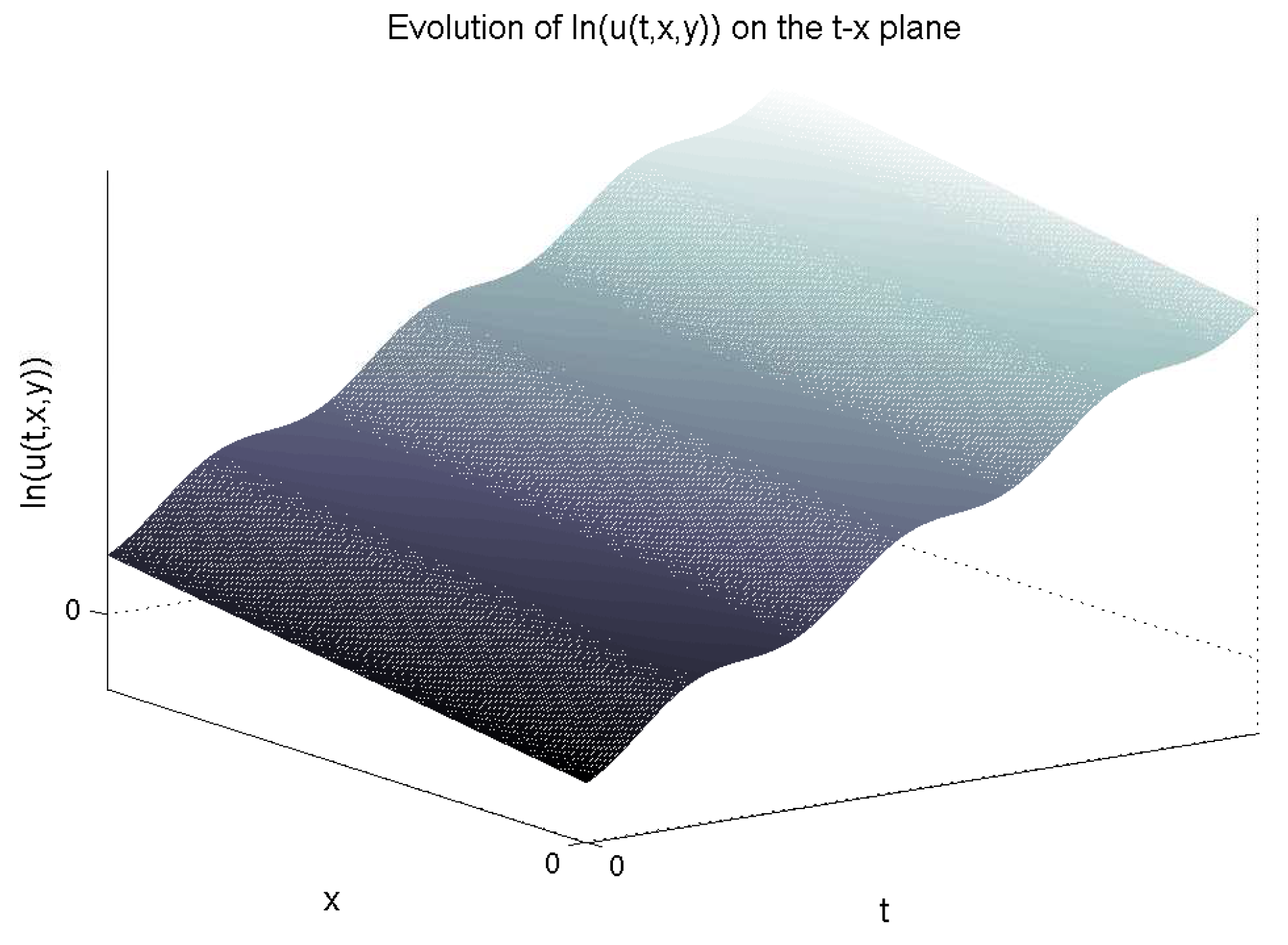
As a final application consider the nonautonomous two-dimensional BS Equation (53). From the application of the invariant functions of the Lie symmetries $\left\{Z_1+c_1{X}_u,Z_3+c_2{X}_u\right\}$ we have the solution $u\left(t,x,y\right)=w\left(t\right)exp\left(c_{1}x+c_{2}y\right)$, where

$$w\left(t\right)=exp\left(\frac{1}{2}\int \left(2k\left(t\right)-\left(c_1^2+c_2^2\right)+{\mathsf{\Lambda }}_1\left(t\right)c_1+{\mathsf{\Lambda }}_2\left(t\right)c_2\right)dt\right)$$

(68)

In the case for which ${\mu }_1\left(t\right)={\mu }_2\left(t\right)=k\left(t\right)=r\left(t\right)$ and $r\left(t\right)=r_0+\epsilon sin\left(\omega t\right)$, ω, ε and $r_0$ are constants, the solution of the nonautonomous two-dimensional BS equation for the “$t-x$” plane is given in Figure 1. We observe that in the $t-$direction, function $u\left(t,x,y\right)$ has periodic behavior along the line $f\left(t\right)\simeq t$ with period ω.

The implication of the results of the present analysis is that for the two-factor model of commodities, the autonomous and the nonautonomous problem share the same static solutions, that is, the differences follow only from the time-dependent terms of the solution. However, that is not true for the two-dimensional Black-Scholes Equation in which the nonautonomous equation in general is not maximally symmetric and does not share the same number of static solutions with that of the autonomous equation. On the other hand we found that if and only if the time-dependence of the two volatilities ${\sigma }_1\left(t\right),{\sigma }_2\left(t\right)$ are the same, i.e., $\frac{{\sigma }_1\left(t\right)}{{\sigma }_2\left(t\right)}=const$, and if the correlation factor ρ is constant then the nonautonomous Black-Scholes shares the same static solutions, i.e., static evolution, with the autonomous equation.

The results of this analysis are important in the sense that by starting from the autonomous equation and with the use of coordinate transformations and only someone can analyse models with time-varying constants. On the other hand starting from real data and with the use of coordinate transformations to see if the data are well described from the autonomous system, and vice verca. The situation is not different from that which one finds on the relation between the free particle and harmonic oscillator. In order to demonstrate that, if we plot the time-position diagram of the mathematical pendulum, where we measure the distance and the time with nonlinear instruments, the graph will be a straight line, which describes the motion of the free particle.

In a forthcoming work we intend to extend our analysis to the case where the free parameters of the models are space-dependent. Such an analysis is in progress and will be published elsewhere.