Lie Symmetry Analysis of the Black-Scholes-Merton Model for European Options with Stochastic Volatility

Abstract

We perform a classification of the Lie point symmetries for the Black-Scholes-Merton Model for European options with stochastic volatility, σ, in which the last is defined by a stochastic differential equation with an Orstein-Uhlenbeck term. In this model, the value of the option is given by a linear (1 + 2) evolution partial differential equation in which the price of the option depends upon two independent variables, the value of the underlying asset, S, and a new variable, y. We find that for arbitrary functional form of the volatility, $\sigma \left(y\right)$, the (1 + 2) evolution equation always admits two Lie point symmetries in addition to the automatic linear symmetry and the infinite number of solution symmetries. However, when $\sigma \left(y\right)={\sigma }_0$ and as the price of the option depends upon the second Brownian motion in which the volatility is defined, the (1 + 2) evolution is not reduced to the Black-Scholes-Merton Equation, the model admits five Lie point symmetries in addition to the linear symmetry and the infinite number of solution symmetries. We apply the zeroth-order invariants of the Lie symmetries and we reduce the (1 + 2) evolution equation to a linear second-order ordinary differential equation. Finally, we study two models of special interest, the Heston model and the Stein-Stein model.

1. Introduction

The Black-Scholes-Merton Model for European options is based upon some Ansatz for the stock price. Specifically, the process for the stock price is characterized by continuity, and it has the ability to hedge continuously with transaction costs and has constant volatility [1,2,3].

In the Black-Scholes-Merton Model, the price of a financial asset is given by the soluton of the stochastic differential equation

$$d{S}_t=r{S}_{t}dt+\sigma S_{t}d{W}_t$$

(1)

where $W_t$ is a Brownian motion, and the value $u=u\left(t,S\right)$ of the option is given by the solution of the $(1+1)$ evolution equation,

$$\frac{1}{2}{\sigma }^2{S}^2{u}_{,SS}+rS{u}_{,S}-ru+u_{,t}=0$$

(2)

in which t is time, S is the current value of the underlying asset, for example a stock price, and r is the rate of return on a safe investment. The value of the option is subject to the satisfaction of the terminal condition, $u\left(T,S\right)=U\left(S\right)$, when $t=T$. Finally, σ is the volatility of the model.

The Black-Scholes-Merton Model assumes constant volatility σ. However, in real problems, σ is not a constant. One possible generalisation of the model, Equation (2), is to consider that the volatility depends upon the time, t, and on the value of the stock, S, i.e., $\sigma =\sigma \left(t,S\right)$. It has been proposed that σ is a function of a mean Orstein–Uhlenbeck process [4].

Consider that $\sigma =f\left(y\right)$, where y is given by the stochastic differential equation with the Orstein–Uhlenbeck term [5,6,7]:

$$d{y}_t=\alpha \left(m-y_t\right)dt+\beta d{\widehat{Z}}_t$$

(3)

The new Brownian motion ${\widehat{Z}}_t$ can be correlated with $W_t$ and be expressed as follows:

$${\widehat{Z}}_t=\rho W_t+\sqrt{1-{\rho }^2}{Z}_t$$

(4)

in which $Z_t$ describes a Brownian motion independent of $W_t$ and ρ is the correlation factor with values $\left|\rho \right|\le 1$.

Hence, the Black-Scholes Equation (2) in the case of stochastic volatility is modified and the value u of the option is given by the $(1+2)$ evolution equation

$$\left({\widehat{M}}_1+{\widehat{M}}_2+{\widehat{M}}_3+{\widehat{M}}_4\right)u\left(t,S,y\right)=0$$

(5)

where the operators, ${\widehat{M}}_1,$ ${\widehat{M}}_2,{\widehat{M}}_3,{\widehat{M}}_4,$ are defined as follows:

$${\widehat{M}}_1=\frac{1}{2}{f}^2\left(y\right)S^2\frac{{\partial }^2}{\partial S^2}+rS\frac{\partial }{\partial S}-r+\frac{\partial }{\partial t}$$

(6)

$${\widehat{M}}_2=\rho \beta Sf\left(y\right)\frac{{\partial }^2}{\partial S\partial y},{\widehat{M}}_3=-\beta \Lambda \left(t,S,y\right)\frac{\partial }{\partial y},\mathrm{and}$$

(7)

$${\widehat{M}}_4=\frac{1}{2}{\beta }^2\frac{{\partial }^2}{\partial y^2}+\alpha \left(m-y\right)\frac{\partial }{\partial y}$$

(8)

The function $\Lambda \left(t,S,y\right)$ is

$$\Lambda \left(t,S,y\right)=\rho \frac{\mu -r}{f\left(y\right)}+\gamma \left(t,S,y\right)\sqrt{1-{\rho }^2}$$

(9)

and $u\left(t,S,y\right)$ satisfies the terminal condition $u\left(T,S,y\right)=U\left(S\right)$ at time $t=T$.

The operator ${\widehat{M}}_1$ gives the Black-Scholes-Merton Equation (2) with volatility $\sigma =f\left(y\right)$, ${\widehat{M}}_2$ expresses the correlation term between the two Brownian motions, $W_t$ and ${\widehat{Z}}_t$, of the European option and of the volatility, respectively, and ${\widehat{M}}_4$ is the Orstein-Uhlenbeck process term. Finally. the term ${\widehat{M}}_3$, the so called premium term, expresses the market price of the volatility risk [6]. The function $\gamma \left(t,S,y\right)$ in Equation (9) is the risk-premium factor which drives the volatility and follows from the second Brownian motion, $Z_t$, where in the case of absolute correlation, i.e., $\left|\rho \right|=1$, $\gamma \left(t,S,y\right)$ does not play any role in the model. The first term of the rhs side of Equation (9) is called the excess return-to-risk ratio [6]. The statistical importance of stochastic volatility has been confirmed in [8].

The purpose of this work is the study of the Black-Scholes-Merton Model with stochastic volatility, Equation (5), by using the method of group invariant transformations, specifically the Lie (point) symmetries of the equation. The importance of Lie symmetries is that they provide a systematic method to facilitate the solution of differential equations because they provide first-order invariants which can be used to reduce the differential equations. Moreover, Lie symmetries can be used for the classification of differential equations. Furthermore, we can extract important information for the differential equation, consequently for the model, from the group of invariant transformations admitted.

The first application of the Lie symmetries in financial modeling was performed by Gazizov & Ibragimov in [9]. They studied the admitted group of invariant transformations for the Black-Scholes-Merton Equation (2), with constant volatility and they proved that Equation (2) admits as Lie symmetries the elements of Lie algebra, $\left\{A_{3,8}{\oplus }_s{A}_{3,1}\right\}{\oplus }_s\infty A_1$ ( In the Mubarakzyanov Classification Scheme [10,11,12,13]). This means that Equation (2) is maximally symmetric and according to the Theorem of Sophus Lie [14] there exists a transformation on the space of variables $\left\{t,S,u\right\}$ in which Equation (2) can be written in the form of the heat equation. The last was an important result because the mathematical methods from physical science can be used for the study of differential equations in financial mathematics. A similar result has been found for the one-factor model of commodities [15], which means that the three different equations, the heat equation, the Black-Scholes-Merton equation and the one-factor model of commodities equation, are equivalent at the mathematical level even if they describe different subjects.

In recent years, Lie symmetries have covered a big range of applications in financial mathematics. For instance, the group invariants of the Cox-Ingersoll-Ross Pricing Equation have been studied in [16] and the nonlinear Merton model in [17]. As far as concerns the Asian option, a Lie symmetry classification has been performed in [18]. As for generalisations of the Black-Scholes-Merton Model, the Lie symmetries and the reduction process of the nonautonomous model can be found in [19,20], while another generalisation of Equation (2) with a “source” was studied in [21].

Furthermore, in [22,23], the symmetry analysis of the space- and time-dependent one-factor model of commodities and of the nonautonomous two-dimensional Black-Scholes-Merton Equations were performed. For other applications of Lie symmetries in financial mathematics, see, for instance, [24,25,26], and references therein.

The stochastic volatility model, Equation (5), is a $(1+2)$ evolution equation. Below, we perform a symmetry analysis and we determine the group invariant solutions. In particular, we restrict our analysis to the model in which the risk premium factor vanishes without necessarily $\left|\rho \right|=1$ and from Equation (9), only the term which expresses the return-to-risk ratio survives. Moreover, we study two models for European options with stochastic volatility, the Heston model [27] and the Stein–Stein model [28]. The latter is a model without correlation between the two Brownian motions, $W_t$ and ${\widehat{Z}}_t,$ i.e., $\rho =0$ in Equation (4). The plan of the paper is as follows.

In Section 2, we give the basic properties and definitions for the Lie point symmetries of differential equations and we perform the symmetry classification for our model. We find that Equation (5) without the risk premium factor is always invariant under the $\left\{3A_1\right\}oplu{s}_s\infty A_1$ Lie algebra. However, when $f\left(y\right)$ is constant, Equation (5) is invariant under a larger Lie algebra. The application of the Lie symmetries to Equation (5) can be found in Section 3, in which we reduce the $\left(1+2\right)$ evolution equation by using the zeroth-order invariants provided by the Lie symmetries and we derive invariant solutions. In Section 4 and Section 5 we study two models of stochastic volatility for European options, the Heston model and the Stein-Stein model, respectively. For these two models, we find that both are invariant under the Lie algebra $\left\{3A_1\right\}{\oplus }_s\infty A_1$, and we apply the Lie symmetries to solve the equations of the two models. For the Heston model, the closed-form solution is expressed in terms of Kummer Functions, whereas for the Stein–Stein model, the closed-form solution is expressed in terms of Hypergeometric Functions. Furthermore, we give some numerical solutions for the two models. Finally, in Section 6, we discuss our results and draw our conclusions

2. Lie Symmetry Analysis

We consider the Black-Scholes-Merton Equation with stochastic volatility governed by the evolution Equation (5) for which the premium term depends only upon the return-to-risk ratio. For a time-independent rate-of-return, Equation (5) becomes

$$\begin{array}{ccc}\mathcal{H}& :& 0=\frac{1}{2}{f}^2\left(y\right)S^2{u}_{,SS}+\rho \beta Sf\left(y\right)u_{,Sy}+\frac{1}{2}{\beta }^2{u}_{,yy}\hfill \\ & & +rS{u}_{,S}+\left[\alpha \left(m-y\right)-\beta \rho \frac{\mu -r}{f\left(y\right)}\right]u_{,y}-ru+u_{,t}\hfill \end{array}$$

(10)

Let Φ be the map of an one-parameter point transformation such as

$$\Phi \left(u\left(t,S,y\right)\right)=u^{\prime }\left(t^{\prime },S^{\prime },y^{\prime }\right)$$

(11)

with infinitesimal transformation (ε is the parameter of smallness.)

$$\begin{array}{ccc}{t}^{\prime }& =& t+\epsilon {\xi }^1\left(t,S,y,u\right)\hfill \end{array}$$

(12)

$$\begin{array}{ccc}{S}^{\prime }& =& S+\epsilon {\xi }^2\left(t,S,y,u\right)\hfill \end{array}$$

(13)

$$\begin{array}{ccc}{y}^{\prime }& =& y+\epsilon {\xi }^3\left(t,S,y,u\right)\hfill \end{array}$$

(14)

$$\begin{array}{ccc}{u}^{\prime }& =& u+\epsilon \eta \left(t,S,y,u\right)\hfill \end{array}$$

(15)

and generator

$$X=\frac{\partial t^{\prime }}{\partial \epsilon }{\partial }_t+\frac{\partial S^{\prime }}{\partial \epsilon }{\partial }_S+\frac{\partial y^{\prime }}{\partial \epsilon }{\partial }_y+\frac{\partial u^{\prime }}{\partial \epsilon }{\partial }_u$$

(16)

Consider now that $u\left(t,S,y\right)$ is a solution of Equation (10) and under the map Φ, Equation (11), $u^{\prime }\left(t^{\prime },S^{\prime },y^{\prime }\right)$ is also a solution of Equation (10). Then, we say that the generator $X,$ of the infinitessimal transformation of the one-parameter point transformation, Φ, is a Lie (point) symmetry of (Equation 10) and Equation (10) is invariant under the action of the map Φ. That means that there exists a function ψ such that the following condition holds [29]

$$X^{\left[2\right]}\left(\mathcal{H}\right)=\psi \mathcal{H},mod\left(\mathcal{H}\right)=0$$

(17)

or, equivalently,

$$X^{\left[2\right]}\left(\mathcal{H}\right)=0$$

(18)

where $X^{\left[2\right]}$ is the second prologation/extension of X in the space of variables $\left\{t,S,y,u,u_{,S},u_{,y},u_{,SS},u_{,Sy},u_{yy}\right\}$. Specifically $X^{\left[2\right]}$ is defined from the following formula

$$X^{\left[2\right]}=X+{\eta }_i^A{\partial }_{u^A}+{\eta }_{ij}^A{\partial }_{u_{ij}^A}$$

(19)

where ${\eta }_i^A,{\eta }_{ij}^A$ are given by the relations

$${\eta }_i^A={\eta }_{,i}^A+u_{,i}^B{\eta }_{,B}^A-{\xi }_{,i}^j{u}_{,j}^A-u_{,i}^A{u}_{,j}^B{\xi }_{,B}^j$$

(20)

and

$$\begin{array}{cc}{\eta }_{ij}^A& ={\eta }_{,ij}^A+2{\eta }_{,B(i}^A{u}_{,j)}^B-{\xi }_{,ij}^k{u}_{,k}^A+{\eta }_{,BC}^A{u}_{,i}^B{u}_{,j}^C-2{\xi }_{,\left(i\right|B|}^k{u}_{j)}^B{u}_{,k}^A\hfill \\ & -{\xi }_{,BC}^k{u}_{,i}^B{u}_{,j}^C{u}_{,k}^A+{\eta }_{,B}^A{u}_{,ij}^B-2{\xi }_{,(j}^k{u}_{,i)k}^A-{\xi }_{,B}^k\left(u_{,k}^A{u}_{,ij}^B+2u_{(,j}^B{u}_{,i)k}^A\right)\hfill \end{array}$$

(21)

The importance of the existence of a Lie symmetry for a partial differential equation is that from the associated Lagrange’s system,

$$\frac{d{x}^i}{{\xi }^i}=\frac{d{u}^A}{{\eta }^A}$$

(22)

Zeroth-order invariants, $U^{\left[0\right]}\left(x^k,u^A\right)$, can be determined which can be used to reduce the number of the independent variables of the differential equation.

In the following, we perform a classification of the Lie symmetries of Equation (10). Function $f\left(y\right)$ is defined by the requirement that Equation (10) admit Lie symmetries. The latter requirement can be seen as a geometric selection rule as the Lie symmetries are generated from the elements of the Homothetic Algebra [30] of the (pseudo)Riemannian space, which defines the Laplace operator in the $(1+2)$ evolution Equation (10). In our case, the (pseudo)Riemannian manifold is defined by the Brownian motions, $W_t,{\widehat{Z}}_t,$ of the stock price, S, and of the volatility, $\sigma$, respectively.

Before we proceed with the symmetry analysis, we remark that Equation (10) is a linear equation which means that it always admits the linear symmetry, $X_u=u{\partial }_u$ and the infinite-dinensional abelian subalgebra of solutions, $X_b=b\left(t,S,y\right){\partial }_u$, where function $b\left(t,S,y\right),$ is a solution of the original Equation (10) [31].

2.1. Classification

From the symmetry condition Equation (17), we get a system of thirty-one equations ( for the derivation of the system, we used the symbolic package SYM of Mathematica [32,33]) in which the solution of the system gives the form of the generator Equation (16) of the transformation Equation (11), that transforms solutions into solutions. From the latter system, we have the following results.

For arbitrary function, $f\left(y\right)$, Equation (10) admits the Lie symmetries

$$X_1={\partial }_t,X_2=S{\partial }_S$$

(23)

plus the vector fields $X_u,X_b$. The algebra in which the Lie symmetries form is the $\left\{3A_1\right\}{\oplus }_s\infty A_1$.

When $f\left(y\right)=f_0$, Equation (10) admits the Lie symmetries

$${\overline{X}}_1={\partial }_t,{\overline{X}}_2=S{\partial }_S,{\overline{X}}_3=e^{-\alpha t}{\partial }_y$$

(24)

$${\overline{X}}_4=2f_{0}tS{\partial }_S+2\frac{\beta }{\alpha }{f}_0\rho {\partial }_y+\left(\left(f_0^2-2r\right)t+2lnS\right)u{\partial }_u$$

(25)

$${\overline{X}}_5=e^{\alpha t}\left(2f_0^2\beta \rho S{\partial }_S+{\beta }^2{f}_0{\partial }_y\right)+\left(2\alpha f_0\left(y-m\right)+2\beta \left(\mu -r\right)\right)u{\partial }_u$$

(26)

plus the vector fields $X_u,X_b$. The Lie Brackets of the Lie algebra are given in

Table 1. Lie brackets of the Lie symmetries of Equation (10) for $f\left(y\right)=f_0$.

$\left[{\overline{\mathbf{X}}}_I,{\overline{\mathbf{X}}}_J\right]$	${\overline{\mathbf{X}}}_1$	${\overline{\mathbf{X}}}_2$	${\overline{\mathbf{X}}}_3$	${\overline{\mathbf{X}}}_4$	${\overline{\mathbf{X}}}_5$	${\mathbf{X}}_u$
${\overline{\mathbf{X}}}_1$	0	0	$-a{\overline{X}}_3$	$2f_0^2{\overline{X}}_2+\left(f_0^2-2r\right)X_u$	$\alpha {\overline{X}}_5$	0
${\overline{\mathbf{X}}}_2$	0	0	0	$2X_u$	0	0
${\overline{\mathbf{X}}}_3$	$\alpha {\overline{X}}_3$	0	0	0	$2\alpha f_0{X}_u$	0
${\overline{\mathbf{X}}}_4$	$-2f_0^2{\overline{X}}_2-\left(f_0^2-2r\right)X_u$	$2X_u$	0	0	0	0
${\overline{\mathbf{X}}}_5$	$-a{\overline{X}}_5$	0	$-2\alpha f_0{X}_u$	0	0	0
${\mathbf{X}}_u$	0	0	0	0	0	0

.

We remark that the two-factor model of commodities is invariant under the same algebra of point transformations [15,23]. That is an expected result because the two-factor model of commodities follows from the one-factor model in which the second factor, product, follows an Orstein-Uhlenbeck process. Moreover, as we discussed in the Introduction, the one-factor model is maximally symmetric just like the Black-Scholes-Merton Equation.

On the other hand $f\left(y\right)=f_0$ means that the volatility σ is constant. However, the second Brownian motion, ${\widehat{Z}}_t,$ in the space wherein σ is defined, interacts with the Brownian motion $W_t$ and modifies the Black-Scholes-Merton Model. However, in the case for which the correlation ρ vanishes, i.e., $\rho =0$, Equation (10) is not reduced to Equation (2) but only when the Orstein-Uhlenbeck process is identically zero, that is, $\beta =0,\alpha =0$. Otherwise, the price u depends upon the Orstein-Uhlenbeck process.

We continue with the reduction of Equation (10) by applying the zeroth-order Lie invariants. Furthermore for every reduced equation we study the Lie symmetries.

3. Group Invariant Solutions

In this section, we apply the Lie symmetries in order to reduce Equation (10). We study the two cases, $f\left(y\right)=f_0,$ and $f\left(y\right)$ to be an arbitrary function. In order to perform the reduction and the later equation to give a solution of the original problem, there should be a constraint between the Lie symmetry vector and the terminal condition. However, we perform the reduction without considering the terminal condition at the moment because the initial conditions can be modified from different options. As far as the invariant solutions of the Black-Scholes-Merton Equation (2) are concerned, see [34].

3.1. Arbitrary Function $f\left(y\right)$

For an arbitrary functional form of $f\left(y\right)$, as we saw above, Equation (10) admits three Lie point symmetries in addition to the infinite number of solution symmetries. The last cannot be used for the reduction. Hence, we do not consider them. Moreover, a solution in which u does not depend upon one of the independent variables is not an acceptable solution, that is, the static solution is of no interest. Therefore, we perform reductions with the symmetry vectors $Y_1=X_1+{\kappa }_1{X}_u$,$Y_2=X_1+{\kappa }_2{X}_u$ and $Y_{12}=X_1+c{X}_2+{\kappa }_3{X}_u$.

Reduction with respect to the Lie invariants of the symmetry vector $Y_1$ gives

$$u\left(t,S,y\right)=exp\left[{\kappa }_{1}t\right]v\left(S,y\right)$$

(27)

where $v\left(S,y\right)$ satisfies the equation

$$\begin{array}{ccc}0& =& \frac{1}{2}{f}^2\left(y\right)S^2{v}_{,SS}+\rho \beta Sf\left(y\right)v_{,Sy}+\frac{1}{2}{\beta }^2{v}_{,yy}\hfill \\ & & +rS{v}_{,S}+\left[\alpha \left(m-y\right)-\beta \rho \frac{\mu -r}{f\left(y\right)}\right]v_{,y}-\left(r-{\kappa }_1\right)v\hfill \end{array}$$

(28)

For this equation, we have that except the linear symmetry and the infinite number of solution symmetries (we call them trivial symmetries) the equation admits the vector field $Y_2=S{\partial }_S$, which is a reduced symmetry. Therefore, the application of $Y_2$ to Equation (28) gives the second-order ordinary differential equation

$${\beta }^2{w}_{,yy}+\left[2\alpha \left(m-y\right)+\frac{2\beta }{f\left(y\right)}\left(\rho {\kappa }_2{f}^2\left(y\right)-\mu +r\right)\right]w_{,y}+\left[\left({\kappa }_2^2-1\right)f^2\left(y\right)+2\left(r{\kappa }_2-r+{\kappa }_1\right)\right]w=0$$

(29)

where $w=w\left(y\right)$ and

$$u\left(t,S,y\right)=S^{{\kappa }_2}exp\left[{\kappa }_{1}t\right]w\left(y\right)$$

(30)

Equation (29) is a linear second-order differential equation, and it is well known that it is maximally symmetric and is invariant under the special linear (sl) algebra $sl\left(3,R\right)$ Lie algebra.

Similarly, if we perform a reduction with $Y_2$, the reduced equation admits the Lie Symmetries $X_1$, $X_v,X_b$, and finally the solution is again given by Equation (30) with the constraint Equation (29).

Consider the application of the Lie symmetry vector $Y_{12}$ to Equation (29). We have that

$$u\left(t,S,y\right)=exp\left[k_{3}t\right]v\left(z,y\right),z=Sexp[-ct]$$

(31)

where

$$\begin{array}{ccc}0& =& z^{2}f\left(y\right)v_{,zz}+2\rho \beta f\left(y\right)v_{,zy}+{\beta }^2{v}_{,yy}+2\left(r-c\right)z{v}_{,z}\hfill \\ & & +2\left[\alpha \left(m-y\right)-\beta \rho \frac{\mu -r}{f\left(y\right)}\right]v_{,y}-\left(r-{\kappa }_3\right)v\hfill \end{array}$$

(32)

One can easily find that this equation only admits the Lie symmetry, $z{\partial }_z$, except the trivial symmetries, which is a reduced symmetry. Therefore, the application of the zeroth-order invariants of the symmetry vector $\left(z{\partial }_z+{\kappa }_{4}v{\partial }_v\right)$ in Equation (32) gives solution of the form Equation (30) with the constraint Equation (29).

We continue with the determination of the group invariant solutions for constant $f\left(y\right)$.

3.2. Constant Volatility

For $f\left(y\right)=f_0$, Equation (10) admits six Lie point symmetries, plus the infinite number of solution symmetries. Moreover, Equation (10) is an $(1+2)$ evolution equation, and, in order to reduce it to an ordinary differential equation, we have to apply the zeroth-order invariants of two Lie symmetries. From Table 1, we select reducing Equation (10) by using the following two-dimensional subalgebras $A_I=\left\{Y_1,Y_2\right\}$, $B_I=\left\{Y_2,{\overline{X}}_3+\kappa X_u\right\}$, $B_{II}=\left\{Y_2,{\overline{X}}_5+\kappa X_u\right\}$, $C_I=\left\{{\overline{X}}_3+\kappa X_u,{\overline{X}}_4\right\}$ and $C_{II}=\left\{{\overline{X}}_4,{\overline{X}}_5\right\}.$

The reduction with the subalgebra $A_I$ we studied in the previous subsection and the solution is Equation (30), where now from Equation (29) we have

$$w\left(y\right)=w_1\mathbf{K}\left(-\frac{c_2}{4\alpha },\frac{1}{2},\frac{{\left(\alpha \left(m-y\right)+\frac{c_1}{2}\right)}^2}{\alpha }\right)+w_2\Lambda \left(-\frac{c_2}{4\alpha },\frac{1}{2},\frac{{\left(\alpha \left(m-y\right)+\frac{c_1}{2}\right)}^2}{\alpha }\right)$$

We have that $w_1$ and $w_2$ are constants,

$$c_1=\frac{2\beta }{f_0}\left(\rho {\kappa }_2{f}_0^2-\mu +r\right),c_2=\left[\left({\kappa }^2-1\right)f_0^2+2\left(r{\kappa }_2-r+{\kappa }_1\right)\right]$$

and $\mathbf{K},\Lambda$ are Kummer Functions.

We continue with the application of the remaining subalgebras.

The application of $B_I$ gives

$$u\left(t,S,y\right)=S^{{\kappa }_2}exp\left(\kappa e^{\alpha t}y\right){\varphi }_I\left(t\right)$$

(33)

where ${\varphi }_I\left(t\right)$ is given by the first-order ordinary differential equation

$$2f_0{\varphi }_{I,t}+\left[\left(f_0^3{\kappa }_2+2f_{0}r\right)\left({\kappa }_2-1\right)+2\kappa \beta \left(f_0^2\rho {\kappa }_2-\mu +r+\frac{\alpha \mu f_0}{\beta }\right)e^{\alpha t}+f_0{\beta }^2{\kappa }^2{e}^{2\alpha t}\right]{\varphi }_I=0$$

(34)

with solution

$$ln\left(\frac{{\varphi }_I\left(t\right)}{{\varphi }_{I0}}\right)=-\frac{\left(f_0^2{\kappa }_2+2r\right)}{2}\left({\kappa }_2-1\right)t-\frac{2\kappa \beta }{2\alpha f_0}\left(f_0^2\rho {\kappa }_2-\mu +r+\frac{\alpha \mu f_0}{\beta }\right)e^{\alpha t}-\frac{{\beta }^2{\kappa }^2}{4\alpha }{e}^{2\alpha t}$$

(35)

From the subalgebra $B_{II}$, we find the solution

$$u\left(t,S,y\right)={\varphi }_{II}\left(t\right)S^{{\kappa }_2}exp\left(\frac{\alpha }{{\beta }^2}{y}^2+\left(\frac{\left(\kappa e^{-\alpha t}-2\alpha m\right)}{{\beta }^2{f}_0}-\frac{2\left(r-\mu +\rho {\kappa }_2{f}_0^2\right)}{\beta f_0}\right)y\right)$$

(36)

where ${\varphi }_{II}\left(t\right)$ is given by the expression

$$\begin{array}{ccc}ln\left(\frac{{\varphi }_{II}\left(t\right)}{{\varphi }_{II0}}\right)& =& -\frac{1}{2}\left[\left(f_0^2{\kappa }_2+2r\right)\left({\kappa }_2-1\right)+2\alpha \right]t\hfill \\ & & +\left[-\frac{\kappa }{\alpha {\beta }^2{f}_0^2}\left(\beta \left(r-\mu +\rho {\kappa }_2{f}_0^2\right)+\alpha m{f}_0\right)e^{-\alpha t}+\frac{{\kappa }^2}{4\alpha f_0^2{\beta }^2}{e}^{-2\alpha t}\right]\hfill \end{array}$$

(37)

For the subalgebra $C_I$, we have the invariant solution

$$u\left(t,S,y\right)=S^{\psi \left(t\right)}exp\left(\kappa e^{\alpha t}y\right){\varphi }_{III}\left(t\right)$$

where

$$\psi \left(t\right)=-\frac{\kappa \beta \rho }{\alpha f_{0}t}-\frac{r}{f_0^2}+\frac{1}{2}+\frac{2}{4f_0^{2}t}$$

(38)

and ${\varphi }_{III}\left(t\right)$ is given by the expression

$$\begin{array}{ccc}ln\left(\frac{{\varphi }_{III}\left(t\right)}{{\varphi }_{III0}}\right)& =& -\frac{1}{2}lnt+\frac{\left(2{\rho }^2-\alpha t\right)}{{\alpha }^{2}t}{\beta }^2{\kappa }^2{e}^{2\alpha t}\hfill \\ & & -\frac{\kappa }{2\alpha f_0}{e}^{\alpha t}\left(2\alpha mf+2\beta \left(r-\mu -2\rho r+\frac{\rho }{2}{f}_0^2\right)+\frac{{\left(2r+f_0^2\right)}^2}{8f_0^2}t\right)\hfill \end{array}$$

(39)

Finally, from the subalgebra $C_{II}$, we find the invariant solution

$$u\left(t,S,y\right)=\frac{{\varphi }_{IV}\left(t\right)}{\sqrt{at-2{\rho }^2}}{S}^{\overline{\psi }\left(t,y\right)}exp\left(V\left(t,y\right)\right)$$

(40)

where

$$\overline{\psi }\left(t,y\right)=\frac{4\rho f_{0}a\left(m-y\right)+\beta \left(\alpha \left(f_0^2-2r\right)t-4\rho \left(\mu -r\right)\right)+\alpha {\beta }^2}{2\beta f_0^2\left(\alpha t-2{\rho }^2\right)}$$

(41)

$$V\left(t,y\right)=\left[\frac{{\alpha }^2}{{\beta }^2\left(\alpha t-2{\rho }^2\right)}y-a\frac{2\beta \left(r-\mu +\frac{f_0^2}{2}\rho -2r\rho \right)+2f_0\alpha m}{{\beta }^2{f}_0^2\left(\alpha t-2{\rho }^2\right)}\right]ty$$

(42)

and function ${\varphi }_{IV}\left(t\right)$ is given by the expression

$$\begin{array}{ccc}ln\left(\frac{{\varphi }_{IV}\left(t\right)}{{\varphi }_{IV0}}\right)& =& -\frac{f_0^2\left(8\alpha -4r-f_0^2\right)-4r^2}{8f_0^2\left(\alpha t-2{\rho }^2\right)}\left(\alpha t^2-2{\rho }^{2}t\right)+\frac{{\left(f_0^2-2r\right)}^2}{2f_0^2\alpha \left(\alpha t-2{\rho }^2\right)}{\rho }^4\hfill \\ & & +\frac{2\left(f_0^2-2r^2\right)\left(f_0\alpha m-\beta \left(\mu -r\right)\right)}{f_0^2\alpha \beta \left(\alpha t-2{\rho }^2\right)}{\rho }^3+\frac{\left(4\beta \left(r-\mu \right)+2f_0\alpha m\right)}{{\beta }^2{f}_0\left(\alpha t-2{\rho }^2\right)}m{\rho }^2\hfill \\ & & +\frac{2{\left(\mu -r\right)}^2}{f_0^2\alpha \left(\alpha t-2{\rho }^2\right)}{\rho }^2\hfill \end{array}$$

(43)

In the following section, we study a special model for stochastic volatility which has been proposed by Heston [27].

4. Heston Model

In the Heston model for stochastic volatility the stock price, S, and the volatility, $\sigma =f\left(y\right)$, satisfy the stochastic differential equation given below

$$\begin{array}{ccc}d{S}_t& =& r{S}_{t}dt+S_t\sqrt{Y_t}d{W}_t\mathrm{and},\hfill \end{array}$$

(44)

$$\begin{array}{ccc}d{Y}_t& =& \theta \left(\overline{m}-Y_t\right)dt+\delta \sqrt{Y_t}d{\widehat{Z}}_t\hfill \end{array}$$

(45)

where, in comparison with Equation (1) and Equation (3), we observe that $f\left(y\right)=\sqrt{y}$ and $\beta =\delta \sqrt{y}$. The differential equation which corresponds to that model is

$$\begin{array}{ccc}0& =& \frac{1}{2}Y{S}^2{u}_{,SS}+\rho \delta YS{u}_{,SY}+\frac{1}{2}{\delta }^{2}Y{u}_{,YY}+rS{u}_{,S}\hfill \\ & & +\left(\theta \left(\overline{m}-Y\right)-\lambda Y\right)u_{,Y}-ru+u_{,t}\hfill \end{array}$$

(46)

Before we proceed with the symmetry analysis of Equation (46), we perform the coordinate transformation $Y=y^2$. Then, Equation (46) becomes

$$\begin{array}{ccc}0& =& \frac{1}{2}{y}^2{S}^2{u}_{,SS}+\beta \rho yS{u}_{,Sy}+\frac{1}{2}{\beta }^2{u}_{,yy}+rS{u}_{,S}\hfill \\ & & +\frac{1}{2}\left[c_{1}y+\left(\frac{c_2}{y}\right)\right]u_{,y}-ru+u_{,t}\hfill \end{array}$$

(47)

in which we have made the replacements $\frac{\delta }{2}\to \beta ,c_1=\left(\theta -\lambda \right)$ and $c_2=\theta m-{\beta }^2$. Equation (47) can be compared with Equation (5) for $f\left(y\right)=y$. However, the risk premium factor of Equation (9) is not zero and has absorbed the term of the Orstein–Uhlenbeck process.

From the Lie symmetry condition, Equation (17) for Equation (47) we find that this equation admits the Lie symmetries

$$X_1={\partial }_t,X_2=S{\partial }_S$$

(48)

plus the $X_u,X_b$, that is, Equation (47) is invariant under the Lie algebra $\left\{3A_1\right\}{\oplus }_s\infty A_1$.

We continue with the application of the Lie symmetries in order to reduce Equation (48). We follow the results of Section 3.1, that is, we apply the group invariants of the subalgebra $\left\{Y_1,Y_2\right\}$.

We find that the corresponding invariant solution of Equation (47) is

$$u\left(t,S,y\right)=S^{{\kappa }_2}{e}^{{\kappa }_{1}t}W\left(y\right)$$

(49)

where $W\left(y\right)$ satisfies the linear second-order differential equation:

$${\beta }^2{W}_{,yy}+\left(2{\kappa }_2\beta \rho +c_{1}y+\frac{c_2}{y}\right)W_{,y}+\left(2{\kappa }_1-2r\left(1-{\kappa }_2\right)+y^2\left({\kappa }_2^2-{\kappa }_1^2\right)\right)W=0$$

(50)

the solution in closed form of which is expressed in terms of Kummer Functions.

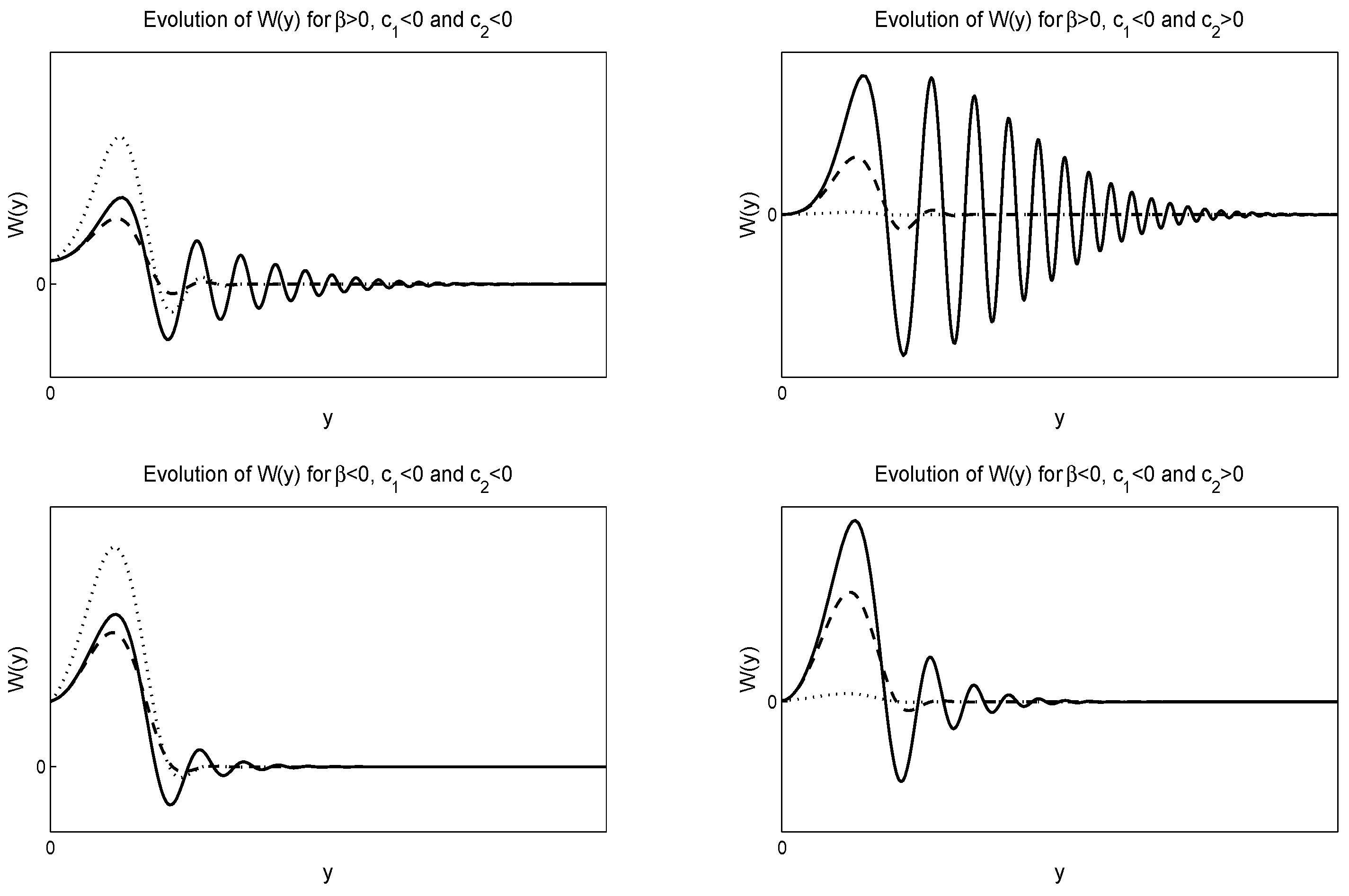
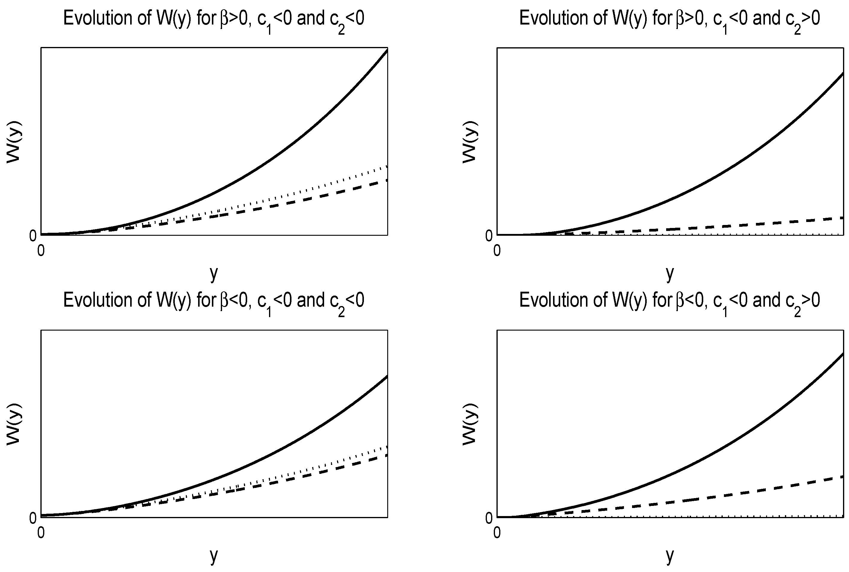
In Figure 1 and Figure 2, we give numerical solutions of Equation (50). Figure 1 is for negative value of $\Delta \kappa ,$whereas Figure 2 is for positive value of $\Delta \kappa$, where $\Delta \kappa ={\kappa }_2-{\kappa }_1$.

5. Stein-Stein Model

The model which has been proposed by Elias M. Stein and Jeremy C. Stein [28] describes an European option with stochastic volatility for which the correlation among the two Brownian motions vanishes, i.e., $\rho =0$, in Equation (4). Moreover, they considered that the risk premium factor is constant, i.e., $\gamma \left(t,S,y\right)={\gamma }_0$ and the volatility is $f\left(y\right)=y$, while the stochastic differential equation is

$$\begin{array}{ccc}d{S}_t& =& r{S}_{t}dt+S_t{Y}_{t}d{W}_t\mathrm{and}\hfill \end{array}$$

(51)

$$\begin{array}{ccc}d{Y}_t& =& \theta \left(\overline{m}-Y_t\right)dt+\delta d{\widehat{Z}}_t\hfill \end{array}$$

(52)

Therefore, from Equation (5), we have that the $(1+2)$ evolution differential equation of the Stein-Stein model is

$$\frac{1}{2}{y}^2{S}^2{u}_{,SS}+\frac{1}{2}{\beta }^2{u}_{,yy}+rS{u}_{,S}+\left[\alpha \left(m-y\right)-\beta {\gamma }_0\right]v_{,y}-ru+u_{,t}=0$$

(53)

From the Lie symmetry condition Equation (17), we find that Equation (53) admits the Lie symmetries

$$X_1={\partial }_t,X_2=S{\partial }_S,X_u=u{\partial }_u,X_b=b\left(t,S,y\right){\partial }_u$$

(54)

which form the Lie algebra $\left\{3A_1\right\}{\oplus }_s\infty A_1$, and it is the admitted algebra of the Heston model and of Equation (10) for the arbitrary function $f\left(y\right)$.

Following the steps of the previous sections, we find that the invariant solution of the Stein–Stein model with respect to the Lie algebra $\left\{Y_1,Y_2\right\}$ is

$$u\left(t,S,y\right)=S^{{\kappa }_2}{e}^{{\kappa }_{1}t}Y\left(y\right)$$

(55)

where $Y\left(y\right)$ is given by the linear second-order differential equation

$${\beta }^2{Y}_{,yy}+\left(2\omega -2ay\right)Y_{,y}+\left(2r\left({\kappa }_2-1\right)+2{\kappa }_1+y^2\left({\kappa }_2^2-{\kappa }_1^2\right)\right)Y=0$$

(56)

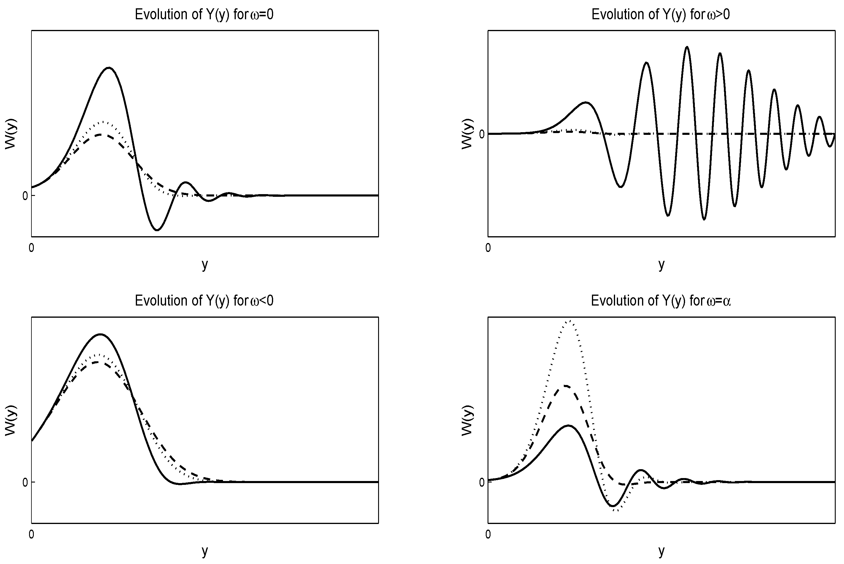
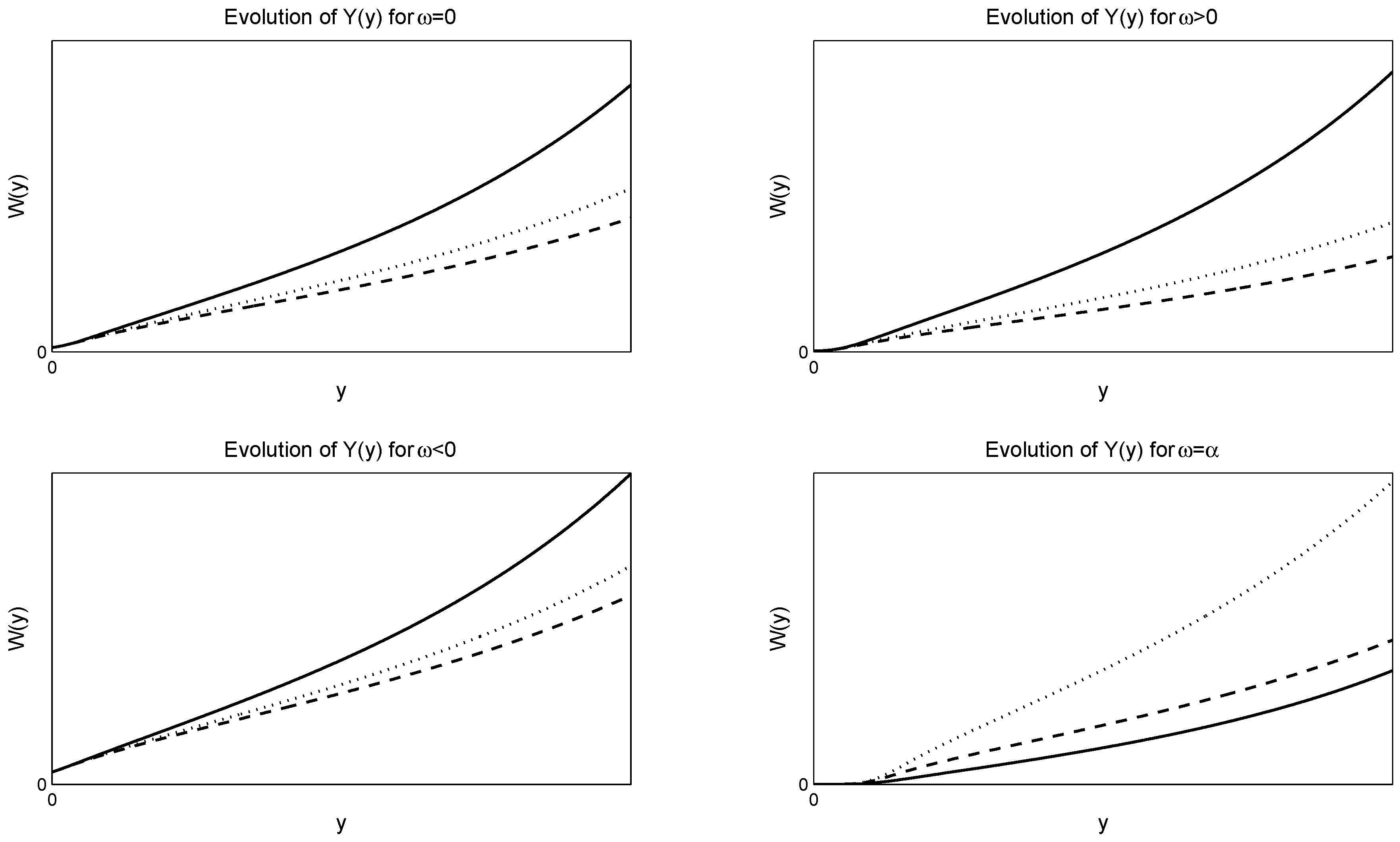
The closed-form solution of this equation can be expressed in terms of the Hypergeometric Functions, where $\omega =\alpha m-\beta {\gamma }_0$. In Figure 3 and Figure 4, we give the numerical evolution of $Y\left(y\right)$ for various values of the parameters, $\omega$and α, for negative $\Delta \kappa$and positive $\Delta \kappa ,$respectively, where $\Delta \kappa ={\kappa }_2-{\kappa }_1$.

6. Conclusions

Volatility with a stochastic process has been shown to be essential for Financial Mathematics. In this work, we studied the algebraic properties, i.e., the Lie symmetries, of the modified Black-Scholes-Merton Equation for European options with a stochastic volatility. We have shown that the autonomous model without the risk premium factor is invariant under a group of point transformations which form the $\left\{3A_1\right\}{\oplus }_s\infty A_1$ Lie Algebra for an arbitrary functional form of the volatility, σ. Moreover, when the volatility is constant but the price of the option depends on the second Brownian motion, in which the volatility is defined, the modified Black-Scholes-Merton Model is invariant under six, plus the infinity, Lie point symmetries and it is not maximally symmetric as theBlack-Scholes-Merton Equation with nonstochastic volatility is.

Furthermore, we showed that the Black-Scholes-Merton Model, in which the volatility is constant, but is defined by an Orstein-Uhlenbeck process, is invariant under the same group of point transformations as that of the two-factor model of commodities. The reason for that is that the two models have in common the terms which follow from the Orstein-Uhlenbeck process.

Moreover, we applied the zeroth-order invariants of the Lie symmetries, and we reduced the model to a linear second-order differential equation. As far as the case of constant volatility is concerned, we found the closed forms of the group invariant solutions.

Finally, we studied the algebraic properties and the invariant solutions of two models, the Heston model and the Stein-Stein model, with stochastic volatility of special interest. For each model, we found the invariant solution and we gave some figures for the evolution of the models. Of course because Equation (5) is a linear equation, the general solution is given by the linear combination of the invariant solutions that we have found, while the latter are constrained by the initial conditions and the boundary conditions of the model.

A general consideration of Equation (5), in which the risk premium factor plays a role is still in progress, and the results will be published elsewhere.

References

1. Black, F.; Scholes, M. The valuation of option contracts and a test of market efficiency. J. Financ. 1972, 27, 399–417. [Google Scholar] [CrossRef]
2. Black, F.; Scholes, M. The pricing of options and corporate liabilities. J. Polit. Econ. 1973, 81, 637–659. [Google Scholar] [CrossRef]
3. Merton, R.C. On the pricing of corporate data: The risk structure of interest rates. J. Financ. 1974, 29, 449–470. [Google Scholar]
4. Sophocleous, C.; O’Hara, J.G.; Leach, P.G.L. Alegbraic solution of the Stein-Stein Model for stochastic volatility. Commun. Nonlinear Sci. Numer. Simul. 2010, 16, 1752–1759. [Google Scholar] [CrossRef]
5. Achdou, Y.; Pironneau, O. Computational Methods for Option Pricing; SIAM USA Philadelphia: Seattle, WA, USA, 2005. [Google Scholar]
6. Fouque, J.P.; Papanicolaou, G.; Sircar, K.R. Derivatives in Financial Markets with Stochastic Volatility; Cambridge University Press: Cambridge, UK, 2000. [Google Scholar]
7. Hull, J.; White, A. The pricing of options on assets with stochastic volatilities. J. Financ. 1987, 42, 281–300. [Google Scholar] [CrossRef]
8. Andersen, T.G.; Benzoni, L.; Lund, J. An empirical investigation of continuous-time equity return models. J. Financ. 2002, 57, 1239–1284. [Google Scholar] [CrossRef]
9. Gazizov, R.K.; Ibragimov, N.H. Lie symmetry analysis of differential equations in Finance. Nonlinear Dyn. 1997, 17, 387–407. [Google Scholar] [CrossRef]
10. Morozov, V.V. Classification of six-dimensional nilpotent Lie algebras. Izv. Vyss. Uchebn Zavendeniĭ Mat. 1958, 5, 161–171. [Google Scholar]
11. Mubarakzyanov, G.M. On solvable Lie algebras. Izv. Vyss. Uchebn Zavendeniĭ Mat. 1963, 32, 114–123. [Google Scholar]
12. Mubarakzyanov, G.M. Classification of real structures of five-dimensional Lie algebras. Izv. Vyss. Uchebn Zavendeniĭ Mat. 1963, 34, 99–106. [Google Scholar]
13. Mubarakzyanov, G.M. Classification of solvable six-dimensional Lie algebras with one nilpotent base element. Izv. Vyss. Uchebn Zavendeniĭ Mat. 1963, 35, 104–116. [Google Scholar]
14. Lie, S. Lectures on Differential Equations with Known Infinitesimal Transformations; Bibliotheca Teubneriana: Leipzig, Germany, 1891. [Google Scholar]
15. Sophocleuous, C.; Leach, P.G.L.; Andriopoulos, K. Algebraic properties of evolution partial differential equations modelling prices of commodities. Math. Methods Appl. Sci. 2008, 31, 679–694. [Google Scholar] [CrossRef]
16. Sinkala, W.; Leach, P.G.L.; O’Hara, J.G. An optimal system and group-invariant solutions of the Cox-Ingersoll-Ross pricing equation. Appl. Math. Comput. 2008, 201, 95–107. [Google Scholar] [CrossRef]
17. Naicker, V.; O’Hara, J.G.; Leach, P.G.L. A note on the integrability of the classical portfolio selection model. Appl. Math. Lett. 2010, 23, 1114–1119. [Google Scholar] [CrossRef]
18. Caister, N.C.; O’Hara, J.G.; Govinder, K.S. Solving the Asian option PDE using Lie symmetry methods. Int. J. Theor. Appl. Financ. 2010, 13, 1256–1277. [Google Scholar] [CrossRef]
19. Sophocleous, C.; Leach, P.G.L. Algebraic aspects of evolution partial differential equations arising in financial mathematics. Appl. Math. Inf. Sci. 2010, 4, 289–305. [Google Scholar]
20. Tamizhmani, K.M.; Krishnakumar, K.; Leach, P.G.L. Algebraic resolution of equations of the Black-Scholes type with arbitrary time-dependent parameters. Appl. Math. Comput. 2014, 247, 115–124. [Google Scholar] [CrossRef]
21. Bozhkov, Y.; Dimas, S. Group classification of a generalized Black-Scholes-Merton equation. Commun. Nonlinear Sci. Numer. Simul. 2014, 19, 2200–2211. [Google Scholar] [CrossRef]
22. Paliathanasis, A.; Morris, R.M.; Leach, P.G.L. The algebraic properties of the space- and time-dependent one-factor problem of commodities. Quaest. Math. 2016. submitted. [Google Scholar]
23. Paliathanasis, A.; Morris, R.M.; Leach, P.G.L. Lie symmetries of (1 + 2) nonautonomous evolution equations in Financial Mathematics. Mathematics 2016. submitted. [Google Scholar]
24. Bozhkov, Y.; Dimas, S. Group classification of a generalization of the Heath equation. Appl. Math. Comput. 2014, 243, 121–131. [Google Scholar] [CrossRef]
25. Okelola, M.O.; Govinder, K.S.; O’Hara, J.G. Solving a partial differential equation associated with the pricing of power options with time-dependent parameters. Math. Methods Appl. Sci. 2015, 38, 2901–2910. [Google Scholar] [CrossRef]
26. Motsepa, T.; Khalique, C.M.; Molati, M. Group classification of a general bond-option pricing equation of mathematical finance. Abstr. Appl. Anal. 2014, 2014, 709871. [Google Scholar] [CrossRef]
27. Heston, S. A closed form solution for options with stochastic volatility with application to bond and currency options. Rev. Financ. Stud. 1993, 6, 327–343. [Google Scholar] [CrossRef]
28. Stein, E.M.; Stein, J.C. Stock-price distributions with stochastic volatility: An analytic approach. Rev. Financ. Stud. 1991, 4, 727–752. [Google Scholar] [CrossRef]
29. Bluman, G.W.; Kumei, S. Symmetries of Differential Equations; Springer-Verlag: New York, NY, USA, 1989. [Google Scholar]
30. Paliathanasis, A.; Tsamparlis, M. Lie point symmetries of a general class of PDEs: The heat equation. J. Geom. Phys. 2012, 62, 2443–2456. [Google Scholar] [CrossRef]
31. Bluman, G.W. Simplifying the form of Lie groups admitted by a given differential equation. J. Math. Anal. Appl. 1990, 145, 52–62. [Google Scholar] [CrossRef]
32. Dimas, S.; Tsoubelis, D. SYM: A new symmetry-finding package for mathematica. In Group Analysis of Differential Equations; Ibragimov, N.H., Sophocleous, C., Damianou, P.A., Eds.; University of Cyprus: Nicosia, Cyprus, 2005; pp. 64–70. [Google Scholar]
33. Dimas, S.; Tsoubelis, D. A new mathematica-based program for solving overdetermined systems of PDEs. In Proceedings of the 8th International Mathematica Symposium, Avignon, France, 19–23 June 2006.
34. Pooe, C.A.; Mahomed, F.M.; Soh, C.W. Invariant solutions of the Black-Scholes equation. Math. Comput. Appl. 2003, 8, 63–70. [Google Scholar]
Figure 1. Evolution of the solution Equation (50) of the Heston model. For the numerical solutions, we select ρ = 0 . 5 , β = 0 . 7 , r = 0 . 5 , κ 1 = 1 and κ 2 = 0 . 5 . The left figures are for negative c 1 , c 2 , while the right figures are for negative c 1 and positive c 2 . The solid lines are for c 2 = 5 c 1 , the dotted lines are for c 2 = 0 . 2 c 1 , and the dash-dash lines are for c 2 = c 1 . The top figures are for β > 0 , while the lower figures for β < 0 .
Mathematics 04 00028 g001
Figure 2. Evolution of the solution Equation (50) of the Heston model. For the numerical solutions, we select ρ = 0 . 5 , β = 0 . 7 , r = 0 . 5 , κ 1 = 1 and κ 2 = 1 . 01 . The left figures are for negative c 1 , c 2 , while the right figures are for negative c 1 and positive c 2 . The solid lines are for c 2 = 3 2 c 1 , the dotted lines are for c 2 = 2 3 c 1 , and the dash-dash lines are for c 2 = c 1 . The top figures are for β > 0 , while the lower figures for β < 0 .
Mathematics 04 00028 g002
Figure 3. Evolution of the solution Equation (56) of the Stein–Stein model. For the numerical solutions, we select β = 0 . 5 , r = 0 . 5 , κ 1 = 1 and κ 2 = 0 . 5 . The figures are for ω = 0 , ω = 0 . 5 , ω = - 0 . 5 and ω = α , respectively. The solid lines are for α = 0 . 1 , the dotted lines are for α = 0 . 3 and the dash-dash lines are for α = 0 . 4 .
Mathematics 04 00028 g003
Figure 4. Evolution of the solution Equation (56) of the Stein–Stein model. For the numerical solutions, we select β = 0 . 5 , r = 0 . 5 , κ 1 = 1 and κ 2 = 1 . 01 . The figures are for ω = 0 , ω = 0 . 5 , ω = - 0 . 5 and ω = α , respectively. The solid lines are for α = 1 . 1 , the dotted lines are for α = 1 . 3 and the dash-dash lines are for α = 1 . 4 .
Mathematics 04 00028 g004