POD-Based Constrained Sensor Placement and Field Reconstruction from Noisy Wind Measurements: A Perturbation Study

Abstract

It is shown in literature that sensor placement at the extrema of Proper Orthogonal Decomposition (POD) modes is efficient and leads to accurate reconstruction of the field of quantity of interest (velocity, pressure, salinity, etc.) from a limited number of measurements in the oceanography study. In this paper, we extend this approach of sensor placement and take into account measurement errors and detect possible malfunctioning sensors. We use the 24 hourly spatial wind field simulation data sets simulated using the Weather Research and Forecasting (WRF) model applied to the Maine Bay to evaluate the performances of our methods. Specifically, we use an exclusion disk strategy to distribute sensors when the extrema of POD modes are close. We demonstrate that this strategy can improve the accuracy of the reconstruction of the velocity field. It is also capable of reducing the standard deviation of the reconstruction from noisy measurements. Moreover, by a cross-validation technique, we successfully locate the malfunctioning sensors.

1. Introduction

Recently, a great effort has been carried out by scientists in developing efficient methods for sensor placement and ocean state reconstruction based on limited measurements that can be used to improve ocean forecasting, at least for regional modelling. One of the efficient methods is the Proper Orthogonal Decomposition (POD), see [1,2,3,4,5], also known as the method of Empirical Orthogonal Functions (EOFs), which have been applied to analyze the measurement data and to develop reconstruction procedures for gappy data sets, see [6,7,8,9,10,11,12,13,14,15,16].

The success of POD approaches depends on a low-dimensional representation of the ocean processes, given the wide spatio-temporal scales, from 1 mm for molecular processes to more than 10 km for fronts, eddies and filaments, and corresponding characteristic times from 1 s to several months ([17]). In [18], the authors showed that only a few spatio-temporal POD modes are sufficient to describe the most energetic ocean dynamics. In particular, they demonstrated that the extrema of the POD spatial modes are very good locations for sensor placement and accurate field reconstruction given a limited number of observing stations and assuming perfect measurements. In [19], the authors proposed to place sensors at extrema but away from each other within a given distance as they found that the extrema of POD spatial modes can be very close and thus produce redundant measurements. See also [20] for a similar approach.

The objective of this paper is to extend the method developed in [19] by investigating the effect of noisy/bad measurements as well as detecting malfunctioning sensors, when POD basis is known. As in [19], we will also impose “declustering” constraints on the sensors as we have observed to avoid redundant measurements at near-by points. Because we use the extrema of the first few modes, empirically, the condition number of the matrix in the linear system of gappy pod method is reduced as shown in [18,19]. We find that this strategy also helps to reduce the reconstruction error. We will consider realistic scenarios, such as measurement uncertainty and bad data from malfunctioning sensor(s). In order to demonstrate the new ideas, we will test our method with the 24 hourly spatial wind field simulation data sets for the Maine Bay. For simplicity, we assume that the noisy measurement data is perturbed by some Gaussian processes. When the perturbation is at the magnitude of the measurements, we assume that the sensor is malfunctioning and thus will be excluded from reconstruction. With a heuristic cross-validation technique, we can locate the malfunctioning sensor effectively.

We remark that there are many other ways to accommodate noise into models and predict the state space from reconstruction—for example, Kalman filtering [21], empirical interpolation method [22,23], and proper generalized decomposition [24,25]. The purpose of our paper is to understand the effect of noisy and bad measurements within the POD framework. Here, we first obtain POD modes from exact complete field and use these POD modes to perform a least square fitting of limited data with the noise in the measurement. This procedure of reconstructing missing or gappy data with POD basis was developed by Everson and Sirovich [26]. While not discussed here, we also note that if the original snapshot ensemble has incomplete data, the POD basis vectors can be computed using an iterative gappy approach [19,27,28]. For bad measurements, we do not perform a Gappy-POD analysis. Instead, we still use the POD modes obtained from the exact field. We alter some measurements of a certain sensor which is regarded as malfunctioning. This is definitely an ideal case for the POD analysis since the bad measurements may significantly change the POD basis. Nevertheless, this ideal testbed provides a basic understanding of the robustness of POD analysis for functioning sensor measurements.

The rest of the paper is organized as follows. In Section 2, we first review the sensor placement strategy based on POD and introduce how to apply an exclusion disk approach to avoid redundant measurements. We discuss in Section 3 the effects of noisy measurements and the effects of exclusion disk approach. In Section 4, we show how to detect a malfunctioning sensor before we summarize and end the paper.

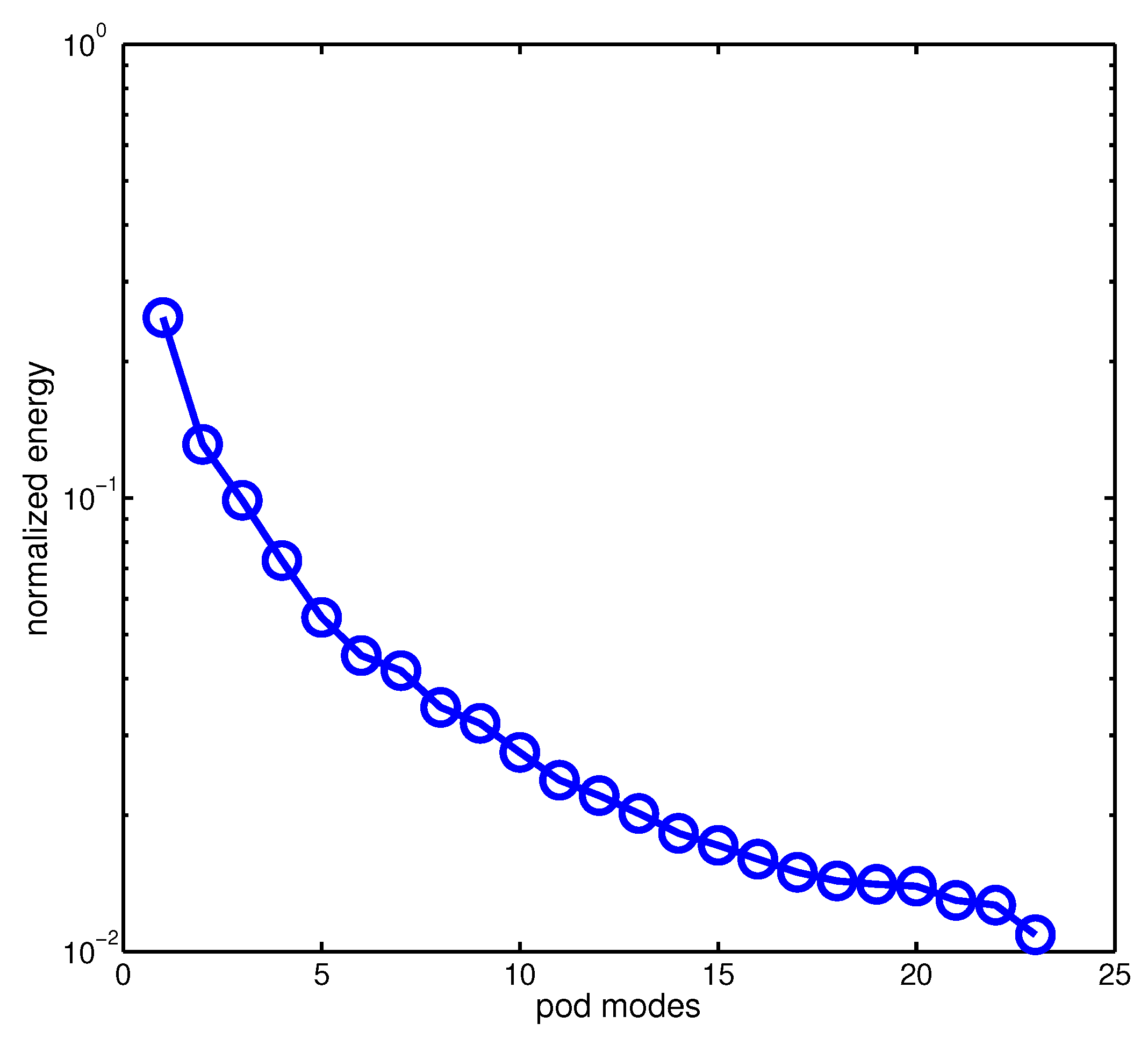
2. A POD-Based Sensor Placement Strategy

The key idea of the POD method is to expand a state variable $u(x,t)$ at certain time t in a spatial domain X as an orthogonal series

$$u\left(x,t\right)=\sum _{k=1}^{\infty }{a}_k\left(t\right){\mathsf{\Phi }}_k\left(x\right),$$

(1)

where ${\mathsf{\Phi }}_k\left(x\right)$’s are orthonormal spatial modes in $L^2\left(X\right)$. Expansion (1) is normally truncated after K terms, which represents the dimensionality of the system. Then, number K is usually small so that we have a low dimensional representation of the process $u(x,t)$ while $\left|\right|u(·,t)-{\sum }_{k=1}^K{a}_k\left(t\right){\mathsf{\Phi }}_k\left|\right|\le ϵ\left|\right|u(·,t)\left|\right|$ and ϵ is small, say $ϵ=0.1$.

In this paper, we will use POD modes obtained from the exact complete field and hence they are “perfect” POD modes. We first review the Gappy-POD before we discuss our sensor placement strategy and the effect of noisy measurements.

2.1. A Review of Gappy-POD

In practice, $u\left(x,t\right)$ may be only obtained at limited locations. To deal with such data (called gappy data), a so-called Gappy-POD was proposed in [7] in order to reconstruct gappy flow fields from a limited number of measurements. As a brief review, we adopt the introduction in [19,27]. Consider a scalar gappy field $\tilde{u}\left(x,t\right)$ as a point-wise product of an indicator function $m\left(x,t\right)$ and a complete field $u\left(x,t\right)$, i.e.,

$$\tilde{u}\left(x,t\right)\stackrel{\mathrm{def}}{=}m\left(x,t\right)u\left(x,t\right).$$

(2)

The indicator function $m\left(x,t\right)$ has values 0 or 1 depending on whether we have data at the corresponding space-time location or not. The goal is to construct a reliable estimator $\widehat{u}\left(x,t\right)$ of $u\left(x,t\right)$ in the space-time regions where $m\left(x,t\right)=0$. In the Gappy-POD framework, it is done applying the method of least-squares: we look for a representation of $\widehat{u}$ in the form

$$\widehat{u}\left(x,t\right)=\sum _{k=1}^K{b}_k\left(t\right){\mathsf{\Phi }}_k\left(x\right),$$

(3)

where ${\mathsf{\Phi }}_k$ are normalized POD spatial modes of $\widehat{u}$ and $b_k$ are unknown coefficients. Note that in practice, ${\mathsf{\Phi }}_k$’s, are extracted from simulation or data assimilation results, and in this paper they are from the perfect model (1). Then, for each snapshot (e.g., each time t), we minimize the approximation error between u and $\widehat{u}$ in the gappy norm

$${∥u-\widehat{u}∥}_m^2\stackrel{\mathrm{def}}{=}{(u-\widehat{u},u-\widehat{u})}_m={\left(u,u\right)}_m-2\sum _{k=1}^K{b}_k{(u,{\mathsf{\Phi }}_k)}_m+\sum _{k=1}^K\sum _{j=1}^K{b}_k{b}_j{({\mathsf{\Phi }}_k,{\mathsf{\Phi }}_j)}_m,$$

(4)

where the (gappy) inner product ${(·,·)}_m$ is defined as

$${\left(a,b\right)}_m\stackrel{\mathrm{def}}{=}{\int }_{X}m\left(x,t\right)a\left(x\right)b\left(x\right)dX,\forall a,b\in L^2\left(X\right).$$

(5)

Minimizing Equation (4) with respect to $b_k$ yields the linear system

$$\mathbf{M}b=f,$$

(6)

where ${\mathsf{M}}_{kj}\stackrel{\mathrm{def}}{=}{({\mathsf{\Phi }}_k,{\mathsf{\Phi }}_j)}_m$ and $f_j\stackrel{\mathrm{def}}{=}{(u,{\mathsf{\Phi }}_j)}_m$. Then, we can obtain time-coefficient vector $b=[b_1\left(t\right),...,b_K\left(t\right)]$ from Equation (6).

Remark 1. 

One should be careful to solve Equation (6) efficiently as the condition number of $\mathbf{M}$ varies with $m(x,t)$. The matrix $\mathbf{M}$ reduces to a $K\times K$ identity matrix in case of complete data, i.e., $m(x,t)=1$. For gappy data, the condition number of $\mathbf{M}$ can be small or large depending on the $m(x,t)$. When the condition number of $\mathbf{M}$ is large, we still formally write Equation (6), but we will solve its corresponding overdetermined system rather than Equation (6). If $\mathbf{M}$ is singular, we seek the pseudoinverse. From now on, we keep this notation and will not state it explicitly.

Based on the aforementioned POD modes and the reconstruction procedure, the authors in [27,29] demonstrated that effective sensor placement strategies can be designed. In this case, the indicator function $m(x,t)$ is defined through sensor locations, i.e., $m(l_j,t)=1$ if there is a (working) sensor at position $l_j$—zero otherwise. The only difference is that the complete field u is now substituted by sensor measurements $d\left(l_j,t\right)$ ($j=1,...,N_s$), where $l_j$ denotes the position of the j-th sensor and $N_s$ is the total number of sensors. The resulting linear system will be also denoted by Equation (6).

In this work, we use the 24 hourly spatial wind field simulation data sets in Maine Bay simulated from the Weather Research and Forecasting (WRF) model. The data we use contain 24 snapshots of the wind field within an area of about 35 km × 25 km from 13 July 2004 00:00 a.m. to 14 July 2004 00:00 a.m. The computation domain and grid are illustrated in Figure 1. The time difference between two successive snapshots is 1 h, namely, snapshot 1 corresponds to data on 13 July 2004 at 0:00 a.m., snapshot 2 corresponds to the data on 13 July 2004 at 1:00 a.m., etc. The temporal average of the window field is subtracted from the field, hence we concentrate on the fluctuation. By cross-correlating different snapshots obtained from the wind simulations, we construct the covariance matrix and its eigen-decomposition. From the eigen-decomposition, we obtain the POD eigenvalues and corresponding hierarchical modes. Here, we use Equations (2)–(6) to obtain Gappy-POD modes. We note that in [27], the procedure Equations (2)–(6) is iterated when the measurement data is incomplete. Here, we focus on complete data but with noise.

In Figure 2, we show the normalized POD eigenvalue spectra of total velocity. For illustration, in Figure 3, we show the contour plots of the first and second POD spatial modes for total velocity.

In case of complete data, e.g., $m(x,t)=\mathbf{1}$, the $L_2$ error of the truncated approximation for each snapshot in Equation (4) is:

$${ϵ}_c\stackrel{\mathrm{def}}{=}{\parallel u-\widehat{u}\parallel }^2={∥\sum _{k=1}^N{a}_k{\mathsf{\Phi }}_k-\sum _{k=1}^K{a}_k{\mathsf{\Phi }}_k∥}^2={∥\sum _{k=K+1}^N{a}_k{\mathsf{\Phi }}_k∥}^2=\sum _{k=K+1}^N{a}_k^2,$$

(7)

due to the orthogonality of ${\mathsf{\Phi }}_k$ and N is the total number of snapshots, i.e., $N=24$. We note that the ${ϵ}_c$ is the lower bound of the error by Gappy-POD method. Since we use gappy data to reconstruct the entire field, the coefficients for the POD models may not be optimal, the coefficients $b_k$’s in Equation (3) are not equal to $a_k$’s in Equation (1). Therefore, the reconstruction error for a fixed snapshot (fixed t) is:

$${ϵ}_g\stackrel{\mathrm{def}}{=}{∥\sum _{k=1}^N{a}_k{\mathsf{\Phi }}_k-\sum _{k=1}^K{b}_k{\mathsf{\Phi }}_k∥}^2={∥\sum _{k=1}^K{a}_k{\mathsf{\Phi }}_k-\sum _{k=1}^K{b}_k{\mathsf{\Phi }}_k∥}^2+{∥\sum _{k=K+1}^N{a}_k{\mathsf{\Phi }}_k∥}^2=\sum _{k=1}^K{(a_k-b_k)}^2+\sum _{k=K+1}^N{a}_k^2.$$

(8)

In [18,19], the authors demonstrate numerically the convergence of the reconstruction error of the Gappy-POD method: ${ϵ}_g$ becomes closer to ${ϵ}_c$ as the number of sensors increases. More specifically, ${\sum }_{k=1}^K{(a_k-b_k)}^2\to 0$ as number of sensors increases. In our data, the first six POD modes ($K=6$) capture more than $90\%$ percent of the total energy. Throughout the paper, we set $K=6$ and we select locations for sensors based on these six modes.

2.2. Constrained Sensor Placement

We first consider the problem of finding the best possible locations where to deploy a limited number of sensors to reconstruct the entire field with existing exact POD modes. Authors in [18,30] demonstrate that the extrema of POD modes are very good locations, when examining reconstruction error in $l_2$ norm, see Equations (10) and (11), to place the sensors for regional ocean forecasting. Yang et al. [19] further introduced the exclusion cylinder to further increase the accuracy of the reconstruction by reducing the redundancy as locations of extrema of different POD modes can be very close. As shown in [19], the exclusion cylinder also helps to reduce the variance of the reconstructed field if the measurement is polluted by the noise. In this paper we employ the exclusion disk instead of the exclusion cylinder for a 2D model. Specially, we impose the following constraint that the distances between each two sensors are larger than R. That is, if we place two sensors at the point $(x_1,y_1)$ and another point $(x_2,y_2)$, then the following restraint is imposed:

$$\sqrt{{(x_1-x_2)}^2+{(y_1-y_2)}^2}>R.$$

(9)

In our wind model, the radius R will be expressed in kilometers. This is achieved by a greedy algorithm: we start with a empty set $F=\varnothing$, then for the next candidate location $(x^{*},y^{*})$ of the sensor (an extrema of a specific mode), we examine whether $\sqrt{{(x^{*}-x_i)}^2+{(y^{*}-y_i)}^2}>R$ holds for each point $(x_i,y_i)$ in F. If not, we neglect this location and examine the next candidate. When a qualified new sensor location $(\tilde{x},\tilde{y})$ is found, we expand F as $F\leftarrow F\cup (\tilde{x},\tilde{y})$.

We distribute the sensors evenly according to the extrema of the POD modes we use to reconstruct the field. In

Table 1. Sensor network configurations in modal space with a fixed number of sensors. A configuration denoted as “4s-4s-4s-4s-4s-4s” with $s=2$ means that we are using 8 sensors in connection with each POD mode from 1 to 6.

Four Modes	Six Modes	Eight Modes
6s-6s-6s-6s	4s-4s-4s-4s-4s-4s	3s-3s-3s-3s-3s-3s-3s-3s

, we provide examples of sensor distribution for a fixed number of sensors with different numbers of POD modes reconstructing the field. With a configuration denoted as “2s-2s-2s-2s” with $s=1$, we distribute 2, 2, 2 and 2 sensors associated with the POD modes 1, 2, 3 and 4, respectively. Similarly a configuration denoted as “4s-4s-4s-4s-4s-4s” with $s=2$ means that we use eight sensors in connection with each POD mode from 1 to 6. Here, we employ this even distribution to demonstrate our idea. The numerical results in [18,19] demonstrate that different configuration of sensor placement will not induce significant difference in the reconstruction.

In our numerical tests, we fix the number of sensors to 24 and use six modes (hence the configuration is “4-4-4-4-4-4”) to reconstruct the entire field to see the effect of the exclusion disk size in reconstructing the total velocity. Figure 4 presents the locations of the sensors with different sizes of the exclusion disk. The contour is for the first POD mode. With larger R, the radius of the disk, the sensors are distributed further away from each other.

Remark 2. 

To avoid redundant measurements, the authors [25] suggested an approach without using the exclusion disk strategy. However, the approach therein only allows one sensor per mode.

To determine the effect of the different exclusion disk size, we define the reconstruction error as (for each flow snapshot)

$$e_i^2\stackrel{\mathrm{def}}{=}\frac{{\displaystyle {\int }_X{({\widehat{U}}_i-U_i)}^{2}dX}}{{\displaystyle {\int }_X{\left(U\right)}_i^{2}dX}},$$

(10)

where $U_i$ is the measurement of total velocity at the i-th snapshot and ${\widehat{U}}_i$ denotes the estimator of the i-th snapshot obtained by solving Equation (6). Here, the integration is performed on the computational domain in physical space. To measure the reconstruction error within the whole period of interest, we also define the time-averaged error as

$$e_{avg}^2\stackrel{\mathrm{def}}{=}\frac{1}{S}\sum _{i=1}^S{e}_i^2,$$

(11)

where S denotes the total number of available snapshots within the considered time interval. The time-averaged error for $R=0,0.5,1,2$ are presented in

Table 2. $e_{avg}^2$ and condition number of M (Cond(M)) for different exclusion disk size R.

R Value	$R=0$	$R=0.5$	$R=1$	$R=2$
$e_{avg}^2$	$17.27\%$	$10.11\%$	$9.26\%$	$9.02\%$
Cond(M)	$83.34$	$22.01$	$16.45$	$10.10$

. Similar to the cases studied in [19] a proper selection of the size of exclusion disk helps to improve the accuracy of the reconstruction. In addition, the size of the exclusion disk need not be very large as we can observe that the error for $R=0.5,1,2$ are quite close. In addition, the condition number of matrix M in Equation (6) decreases as R increases, which is consistent with the results reported in [18,19]. As an illustration, we compare the exact velocity field of the first snapshot (13 July 2004 00:00 a.m.) with those reconstructed with $R=0$ and $R=2$, respectively in Figure 5. It is demonstrated in Figure 5 that the reconstruction of the wind field at the first snapshot is more accurate with the exclusion disk than that without the exclusion disk.

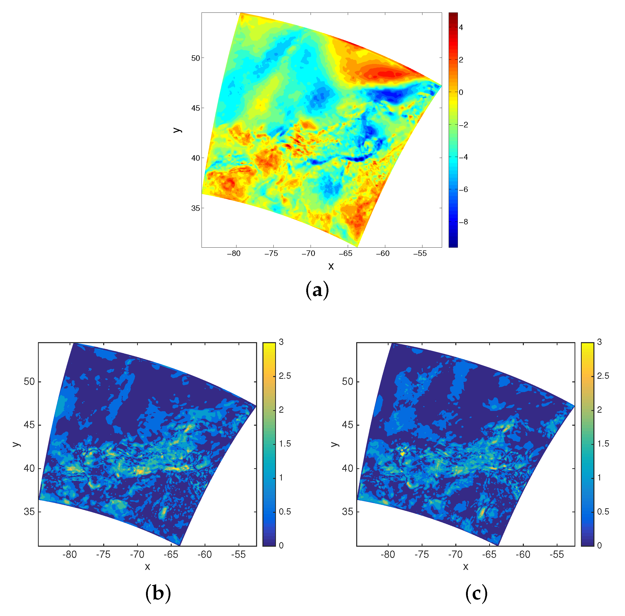
3. Uncertainty in Measurements

In this section, we investigate the uncertainty of the reconstructed field assuming that the sensor signals are perturbed by random noise. Specifically, we assume that the total velocity detected by the sensors has the form

$$d(l_i,t;\xi )=U(l_i,t)+\xi (l_i,t),$$

(12)

where $U(l_i,t)$ is a total velocity to be evaluated and $\xi (l_i,t)$ are $N_s$ i.i.d. zero-mean Gaussian processes with standard deviation ${\sigma }_{\xi }(l_i,t)$. To accommodate the measurement uncertainty, we look for an estimation of the total velocity by random temporal modes and deterministic spatial modes [19,31,32] as:

$$U_{\mathrm{est}}(x,t_j;\xi )=\sum _{k=1}^K{\eta }_k\left(t_j;\xi \right){\mathsf{\Phi }}_k\left(x\right).$$

(13)

Here, ${\mathsf{\Phi }}_k$ are obtained by decomposing full wind field perfect data from Equation (3). The notation $U_{\mathrm{est}}(x,t_j;\xi )$ emphasizes that the stochastic total velocity Equation (13) depends on all random variables

$$\xi \stackrel{\mathrm{def}}{=}[\xi (l_1,t_1),...,\xi (l_{N_s},t_S)],$$

(14)

characterizing the measurement errors. Now, let us consider the following functional (more general data assimilation schemes based on quadratic regularization functionals can be considered).

$$\mathcal{J}\left[{\eta }_k\right]=\langle \sum _{i=1}^{N_s}{[d(l_i,t;\xi )-\sum _{j=1}^K{\eta }_j(t;\xi ){\mathsf{\Phi }}_j\left(l_i\right)]}^2\rangle ,$$

(15)

where $\langle ·\rangle$ denotes an average with respect to the joint probability density of the random vector ξ. Minimization of Equation (15) with respect to ${\eta }_k\left(t;\xi \right)$ yields the following Euler-Lagrange equations

$$\sum _{k=1}^K{\eta }_k(t;\xi )\sum _{i=1}^{N_s}{\mathsf{\Phi }}_k\left(l_i\right){\mathsf{\Phi }}_m\left(l_i\right)=\sum _{i=1}^{N_s}d(l_i,t;\xi ){\mathsf{\Phi }}_m\left(l_i\right).$$

(16)

This system can be recast in same form as Equation (6), i.e.,

$$\sum _{j=1}^K{({\mathsf{\Phi }}_i,{\mathsf{\Phi }}_j)}_m{\eta }_j={(d,{\mathsf{\Phi }}_i)}_m,$$

(17)

provided the gappy inner product Equation (5) is defined in terms of the sensor locations; that is, $m(x,t)=1$ if $x=l_j$—zero otherwise. Denote by ${\mathbf{M}}^{-1}$ the (pseudo)inverse of $\mathbf{M}$, then we obtain a unique solution to Equation (17) in the form

$${\eta }_i(t;\xi )=\sum _{j=1}^K{\left({\mathsf{M}}^{-1}\right)}_{ij}{(d,{\mathsf{\Phi }}_j)}_m.$$

(18)

Next, we calculate the standard deviation of the estimate Equation (13) based statistical assumption of the measurements errors. Specifically, by using the independence hypothesis of the measurement errors, we obtain

$${\sigma }_{U_{\mathrm{est}}}(x,t)\stackrel{\mathrm{def}}{=}\sqrt{\sum _{i=1}^K\sum _{k=1}^K(\langle ({\eta }_i-\langle {\eta }_i\rangle )({\eta }_k-\langle {\eta }_k\rangle )\rangle {\mathsf{\Phi }}_i\left(x\right){\mathsf{\Phi }}_k\left(x\right)},$$

(19)

where we have from Equations (6), (18) and (12) that

$$\begin{array}{ccc}\hfill \langle {\eta }_i\rangle & =& \sum _{j=1}^K{\left({\mathsf{M}}^{-1}\right)}_{ij}{(\langle d\rangle ,{\mathsf{\Phi }}_j)}_m,{\eta }_i-\langle {\eta }_i\rangle =\sum _{j=1}^K{\left({\mathsf{M}}^{-1}\right)}_{ij}{(\xi (l_i,t),{\mathsf{\Phi }}_j\left(x\right))}_m.\hfill \end{array}$$

(20)

Substituting Equations (20) into (19) yields the following final formula

$${\sigma }_{U_{\mathrm{est}}}(x,t)=\sqrt{\sum _{i=1}^K\sum _{k=1}^K\sum _{l=1}^K\sum _{n=1}^K\sum _{j=1}^{N_s}{\sigma }_{\xi }^2(l_j,t){\left({\mathsf{M}}^{-1}\right)}_{il}{\left({\mathsf{M}}^{-1}\right)}_{kn}{\mathsf{\Phi }}_l\left(l_j\right){\mathsf{\Phi }}_n\left(l_j\right){\mathsf{\Phi }}_i\left(x\right){\mathsf{\Phi }}_k\left(x\right)}.$$

(21)

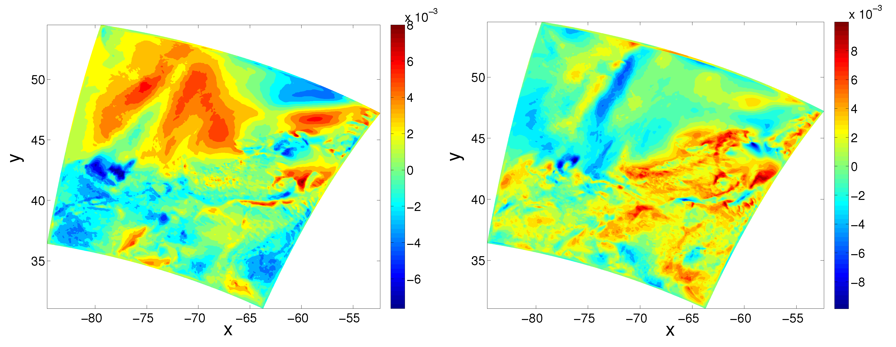
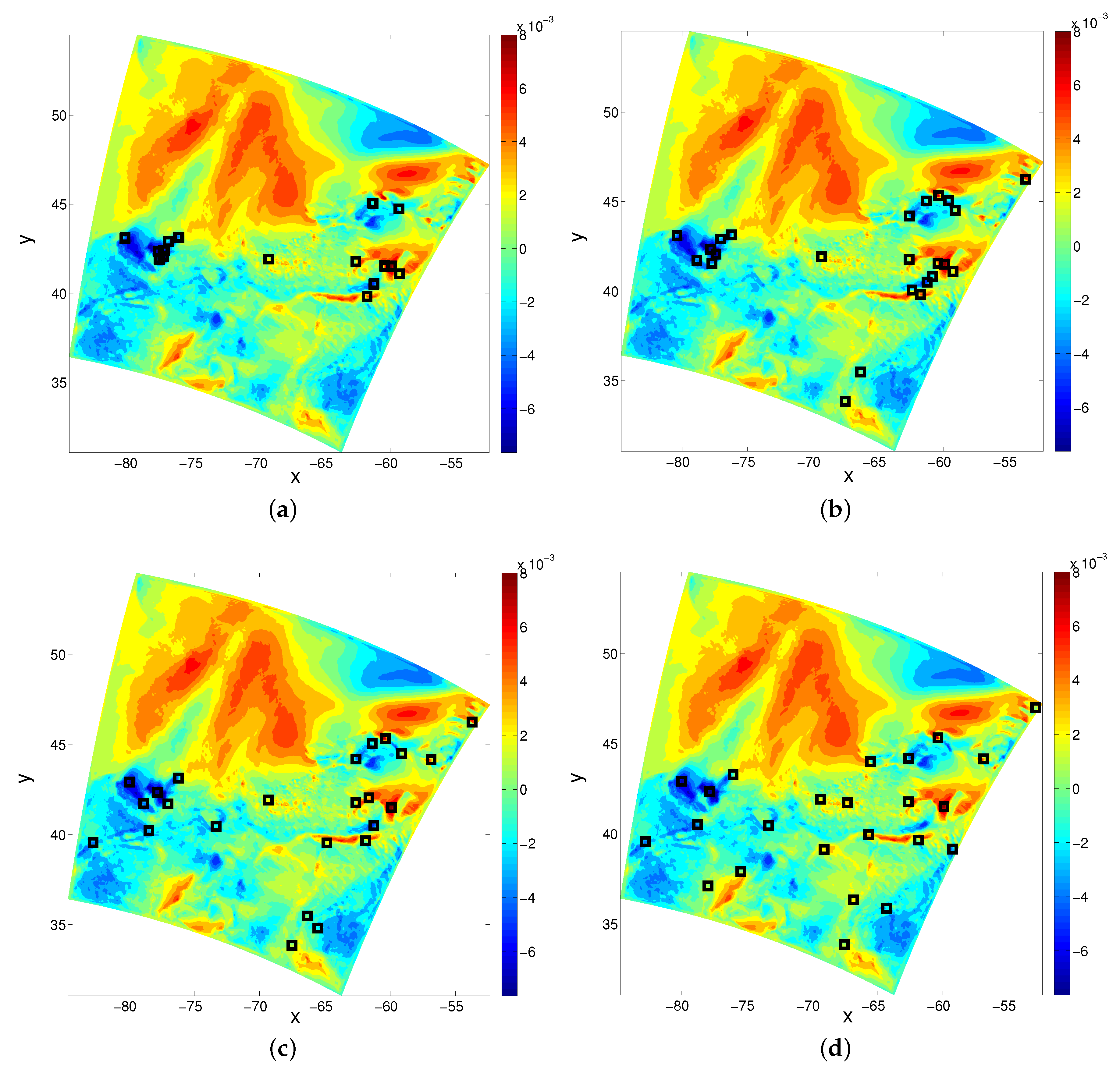
3.1. Results for Uniform Measurement Errors

Let us assume that the standard deviation of the measurement errors is a constant, i.e., ${\sigma }_{\xi }(x,t)={\sigma }_{\xi }$. In this case, Equation (21) simplifies to

$${\sigma }_{U_{\mathrm{est}}}\left(x\right)={\sigma }_{\xi }\sqrt{\sum _{j=1}^{N_s}{\left(\sum _{n=1}^K\sum _{k=1}^K{\left({\mathsf{M}}^{-1}\right)}_{kn}{\mathsf{\Phi }}_n\left(l_j\right){\mathsf{\Phi }}_k\left(x\right)\right)}^2},$$

(22)

yielding to a time-independent standard deviation of the estimate Equation (13).

Figure 6 reports on results of standard deviation calculations given ${\sigma }_{\xi }=1.0$ for different sensor placement strategies. In particular, we fix the POD modes used to reconstruct the field and compare the standard deviation of the reconstructed field with different sizes of exclusion disks. The results of reconstructing the first snapshot are presented. As the reconstructions of all snapshots are similar, we will not present the corresponding results here.

In

Table 3. Average and maximum of ${\sigma }_{U_{\mathrm{est}}}(x,t)$ over all snapshots given ${\sigma }_{\xi }=1$ for different R.

R Value	$R=0$	$R=0.5$	$R=1$	$R=2$
maximum of ${\sigma }_{U_{\mathrm{est}}}(x,t)$	$1.383$	$0.9868$	$0.9305$	$0.6744$
average of ${\sigma }_{U_{\mathrm{est}}}(x,t)$	$0.1781$	$0.1104$	$0.1100$	$0.1031$

, we compare the averages and the maximum of ${\sigma }_{U_{\mathrm{est}}}\left(x\right)$ over all $x$. Numerical results indicate that the exclusion disk method indeed yields smaller standard deviations of the reconstructed field. Clearly, a suitable R helps to reduce the standard deviation Equation (22) in the prediction.

3.2. Results for Non-Uniform Measurement Errors

Next, we study a more realistic case in which the standard deviation of $\xi (x,t)$ is functionally dependent on the total velocity $U(x,t)$. The simplest case is ${\sigma }_{\xi }(x,t)=\alpha U(x,t)$, where α is a positive constant ($U\ge 0$ by construction). From Equation (21), we readily derive the following analytical expression for the standard deviation of $U_{\mathrm{est}}$

$${\sigma }_{U_{\mathrm{est}}}(x,t)=\alpha \sqrt{\sum _{j=1}^{N_s}{U}^2(l_j,t){\left(\sum _{n=1}^K\sum _{k=1}^K{\left({\mathsf{M}}^{-1}\right)}_{kn}{\mathsf{\Phi }}_n\left(l_j\right){\mathsf{\Phi }}_k\left(x\right)\right)}^2}.$$

(23)

Here, we obtain numerical results with a typical value $\alpha =1.0$ corresponding to $100\%$ errors in measuring velocity. We can then compute the average and maximum standard deviation of the estimate $U_{\mathrm{est}}$. As an illustration, the results of these calculations are summarized in Figure 7 for the snapshot 1.

Similarly, the exclusion disk indeed yields smaller standard deviations of the reconstructed as the results shown in

Table 4. Average and maximum of ${\sigma }_{U_{\mathrm{est}}}(x,t)$ over all snapshots given ${\sigma }_{\xi }(l_i,t)=U(l_i,t)$ for different R.

R Value	$R=0$	$R=0.5$	$R=1$	$R=2$
maximum of ${\sigma }_{U_{\mathrm{est}}}(x,t)$	$9.147$	$7.756$	$5.929$	$5.820$
average of ${\sigma }_{U_{\mathrm{est}}}(x,t)$	$1.694$	$1.296$	$1.294$	$1.098$

. Here, the results indicate that suitable R also helps to reduce the standard deviation in the prediction. We note that here ${\sigma }_{U_{\mathrm{est}}}(x,t)$ is linearly dependent on α. For smaller α, the results can be obtained by simply scaling the numbers in Table 4 and the patterns of the distribution of the deviation is the same as those shown in Figure 7. In the next section, we discuss the case that the measurement error from a sensor is considerably large which means the sensor is malfunctioning.

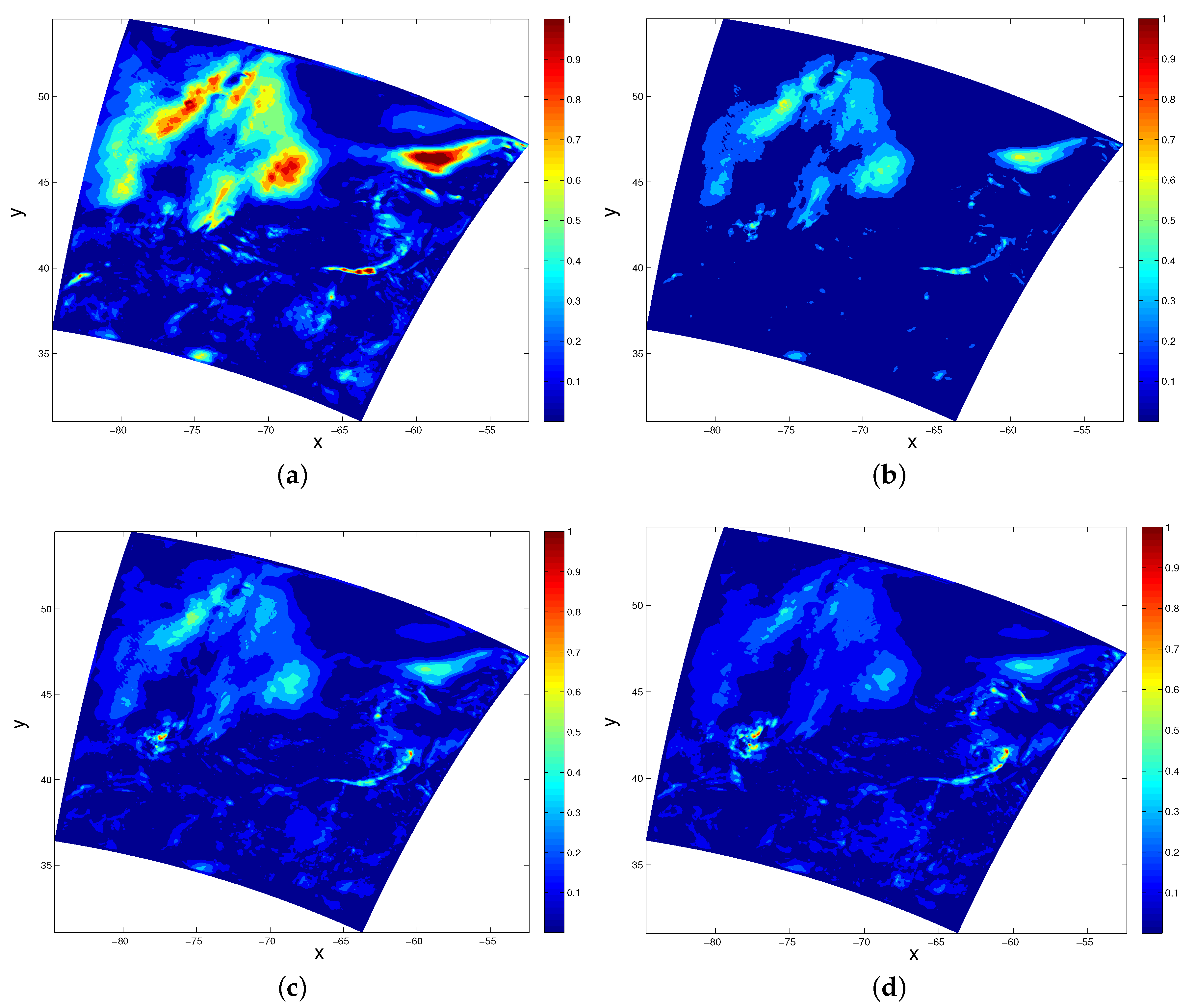
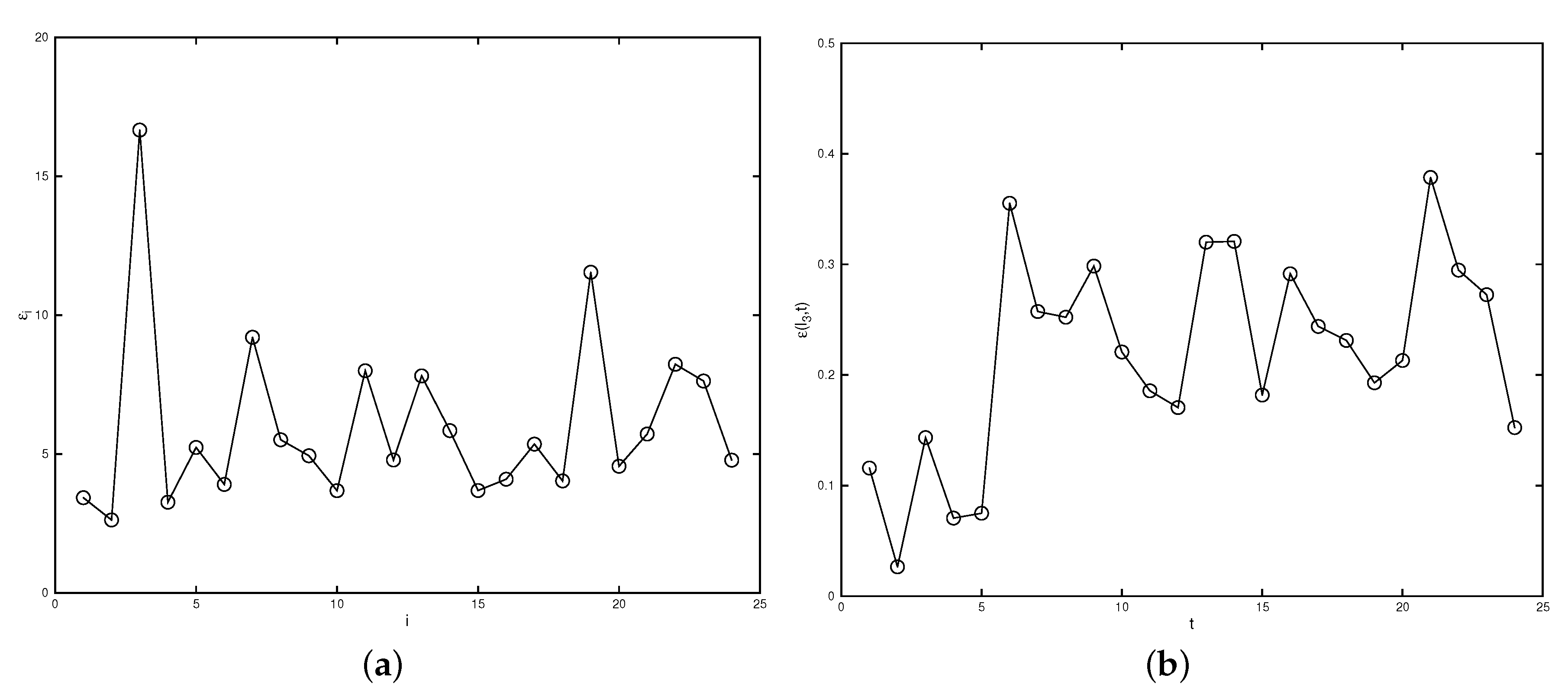
4. Detecting the Malfunctioning Sensor

In this section, we assume that one sensor is not functioning correctly, and all the other sensors provide accurate data. Specifically, we assume that the observed gappy field for each snapshot is $\tilde{u}\left(t\right)=u\left(t\right)+{\delta }_{l^{*}}u\left(t\right)$, where ${\delta }_{l^{*}}u\left(t\right)$ has only one non-zeros entry corresponding to the contaminated sensor at location $l^{*}$. The coefficients $\tilde{b}$ for the POD modes minimize the gappy norm $\parallel \tilde{u}-\tilde{\widehat{u}}{\parallel }_m$, where $\tilde{\widehat{u}}$ is the reconstruction from the Gappy-POD. For each snapshot, given sufficient number of sensors as well as appropriate exclusive disk radius, we have that at each sensor location $l_j$, $|u\left(l_j\right)-\widehat{u}\left(l_j\right){|}^2\sim \mathcal{O}\left({\displaystyle \frac{1}{N_g}}{\sum }_{k=K+1}^N{a}_k^2\right)$, where $N_g$ is the number of grid on the computational domain. Hence, if $|{\delta }_{l^{*}}{u|}^2$ is much larger than $\mathcal{O}\left({\displaystyle \frac{1}{N_g}}{\sum }_{k=K+1}^N{a}_k^2\right)$, we can expect big discrepancy between u and $\widehat{u}$ at $l^{*}$. We thus propose the following heuristic cross-validation method to detect the malfunctioning sensor :

• For each sensor location $l_i$, we use the data from $l_1$, $l_2$, …, $l_{i-1}$, $l_{i+1}$, …, $l_{N_s}$ to reconstruct the field and denote the reconstructed valued at this point as $\widehat{U}(l_i,t)$. Here, we take $N_s=24$ as we consider only the first 24 snapshot from our data.
• Compute the difference between the reconstructed value and the observed value at each $l_i$: $\epsilon (l_i,t_j)=|\widehat{U}(l_i,t_j)-U(l_i,t_j)|$, $j=1,2,\cdots ,N_s$.
• Compare the sum of $\epsilon (l_i,t)$ over all snapshots at each $l_i$. When ${\epsilon }_i=\sqrt{{\sum }_{j=1}^{N_s}{\epsilon }^2(l_i,t_j)}$ is large, we claim that the i-th sensor is not functioning well.

Remark 3. 

The sensors identified by the aforementioned method are candidates for erroneous sensors. Even if only one of the sensors is not working, we can select more than one sensors as candidates for further check. In addition, this method can be applied to the case when more than one sensors are not working.

As a demonstration, we consider a case when $N_s=24$ sensors are located based on the extrema of the first six POD modes with the exclusion disk of radius $R=2.0$. To test our cross-validation method, we perturb the measurement from the third sensor with noise and keep the measurements from the rest of sensors unaltered. Moreover, we consider a scenario that this third sensor is working properly from $t=1$ until $t=5$, then for the remaining time, the error of this sensor is (1) $25\%$ and (2) $50\%$ for our perturbation. We intend to examine whether our method is capable of identifying the malfunctioning sensor. Figure 8a demonstrates that when the error of the sensor is $25\%$, ${\epsilon }_3$ is apparently much larger than other ${\epsilon }_i$, which implies that the third sensor may be malfunctioning (after certain snapshot). By examining $\epsilon (l_3,t)$ for each t as in Figure 8b, we are also able to identify the time when this sensor starts to malfunction. Figure 9 demonstrates similar results when the error of the sensor is $50\%$. Comparing Figure 8 and Figure 9, we observe that when the error becomes larger, the anomaly of this third sensor becomes easier to detect with our approach. Notice that more numerical results (not shown here) imply that the cross-validation method works when any of the sensor is malfunctioning. We select the third sensor to be anomaly only for demonstration purpose.

5. Conclusions

In this work, we extended the exclusion cylinder strategy to sensor placements for reconstructing two-dimensional wind fields. Our numerical tests suggested that a proper size of area exclusion could improve the quality of the field reconstruction from measurements. We addressed the issue of uncertainty in the measurements by adding Gaussian noise in the 24 hourly spatial wind field simulation data sets in Maine Bay simulated from the WRF model that provided the testbed for our work. In particular, we considered two cases: the uncertainty in the measurements is constant everywhere or is varying in space and time. We checked the standard deviation of the reconstructed field and found proper exclusion disk sizes can reduce the errors of the reconstruction filed. With cross-validation techniques, we located a malfunctioning sensor that provides large measurement errors. The numerical results in this paper suggest that the exclusion disk strategy within the Gappy-POD framework can be applied to optimize sensor placements in two-dimensional problems. As future work, we expect to work towards our ultimate goal to develop real-time adaptive sampling for wind forecasting, which helps to find optimal locations for wind turbines with measurements from functioning sensors.

References

1. Venturi, D. On Proper Orthogonal Decomposition of Randomly Perturbed Fields with Applications to Flow past a Cylinder and Natural Convection over a Horizontal Plate. J. Fluid Mech 2006, 559, 215–254. [Google Scholar] [CrossRef]
2. Rempfer, D. Low-dimensional modeling and numerical simulation of transition in simple shear flow. Ann. Rev. Fluid Mech. 2003, 35, 229–265. [Google Scholar] [CrossRef]
3. Bekooz, G.; Holmes, P.; Lumley, J. The proper orthogonal decomposition in the analysis of turbulent flows. Ann. Rev. Fluid Mech. 1993, 25, 539–575. [Google Scholar] [CrossRef]
4. Aubry, N.; Guyonnet, R.; Stone, E. Spatio-temporal analysis of complex signals: Theory and applications. J. Stat. Phys. 1991, 64, 683–739. [Google Scholar] [CrossRef]
5. Sirovich, L. Turbulence and the dynamics of coherent structures, Parts I, II and III. Quart. Appl. Math. 1987, XLV, 561–590. [Google Scholar]
6. Zhang, Y.; Bellingham, J. An efficient method of selecting ocean observing locations for capturing the leading modes and reconstructing the full field. J. Geophys. Res. 2008, 113, C04005. [Google Scholar] [CrossRef]
7. Venturi, D.; Karniadakis, G. Gappy Data and Reconstruction Procedures for Flow Past a Cylinder. J. Fluid Mech. 2004, 519, 315–336. [Google Scholar] [CrossRef]
8. Alvera-Azcárate, A.; Barth, A.; Rixen, M.; Beckers, J.M. Reconstruction of incomplete oceanographic data sets using empirical orthogonal functions: Application to the Adriatic Sea surface temperature. Ocean Modelling 2005, 9, 325–346. [Google Scholar] [CrossRef] [Green Version]
9. Beckers, J.; Rixen, M. EOF Calculations and Data Filling from Incomplete Oceanographic datasets. J. Atmos. Ocean Tech. 2003, 20, 1839–1856. [Google Scholar] [CrossRef]
10. D’Andrea, F.; Vautard, R. Extratropical low-frequency variability as a low dimensional problem. Part I: A simplified model. Quart. J. Roy. Meteor. Soc. 2001, 127, 1357–1375. [Google Scholar] [CrossRef]
11. Hendricks, J.; Leben, R.; Born, G.; Koblinsky, C. Empirical orthogonal function analysis of global TOPEX/POSEIDON altimeter data and implications for detection of global sea rise. J. Geophys. Res. 1996, 101, 14131–14145. [Google Scholar] [CrossRef]
12. Everson, R.; Cornillon, P.; Sirovich, L.; Webber, A. An empirical eigenfunction analysis of sea surface temperatures in the North Atlantic. J. Phys. Ocean. 1995, 27, 468–479. [Google Scholar] [CrossRef]
13. Wilkin, J.; Zhang, W. Modes of mesoscale sea surface height and temperature variability in the East Australian Current. J. Geophys. Res. 2006, 112, C01013. [Google Scholar] [CrossRef]
14. Pedder, M.; Gomis, D. Application of EOF Analysis to the spatial estimation of circulation features in the ocean sampled by high-resolution CTD samplings. J. Atmos. Ocean Tech. 1998, 15, 959–978. [Google Scholar] [CrossRef]
15. Houseago-Stokes, R. Using optimal interpolation and EOF analysis on North Atlantic satellite data. International WOCE Newsletter 2000, 28, 26–28. [Google Scholar]
16. Preisendorfer, W.; Mobley, C.D. Principal component analysis in meteorology and oceanography; Elsevier: Amsterdam, The Netherlands, 1988. [Google Scholar]
17. Dickey, T. Emerging ocean observations for interdisciplinary data assimilation systems. J. Mar. Syst. 2003, 40–41, 5–48. [Google Scholar] [CrossRef]
18. Yildirim, B.; Chryssostomidis, C.; Karniadakis, G.E. Efficient sensor placement for ocean measurement using low-dimensional concepts. Ocean Modelling 2009, 27, 160–173. [Google Scholar] [CrossRef]
19. Yang, X.; Venturi, D.; Chen, C.; Chryssostomidis, C.; Karniadakis, G.E. EOF-based constrained sensor placement and field reconstruction from noisy ocean measurements: Application to Nantucket Sound. J. Geophys. Res. 2010, 115. [Google Scholar] [CrossRef]
20. Xue, P.; Chen, C.; Beardsley, R.C.; Limeburner, R. Observing system simulation experiments with ensemble Kalman filters in Nantucket Sound, Massachusetts. J. Geophys. Res. Oceans 2011, 116. [Google Scholar] [CrossRef]
21. Li, W.; Sun, S.; Jia, Y.; Du, J. Robust unscented Kalman filter with adaptation of process and measurement noise covariances. Digit. Signal Process. 2016, 48, 93–103. [Google Scholar] [CrossRef]
22. Barrault, M.; Maday, Y.; Nguyen, N.C.; Patera, A.T. An ’empirical interpolation’ method: Application to efficient reduced-basis discretization of partial differential equations. Comptes Rendus Mathematique 2004, 339, 667–672. [Google Scholar] [CrossRef]
23. Chaturantabut, S.; Sorensen, D.C. Nonlinear model reduction via discrete empirical interpolation. SIAM J. Sci. Comput. 2010, 32, 2737–2764. [Google Scholar] [CrossRef]
24. Chinesta, F.; Leygue, A.; Bordeu, F.; Aguado, J.; Cueto, E.; González, D.; Alfaro, I.; Ammar, A.; Huerta, A. PGD-based computational vademecum for efficient design, optimization and control. Arch. Comput. Methods Eng. 2013, 20, 31–59. [Google Scholar] [CrossRef]
25. Nadal, E.; Chinesta, F.; Díez, P.; Fuenmayor, F.; Denia, F. Real time parameter identification and solution reconstruction from experimental data using the Proper Generalized Decomposition. Comput. Methods in Appl. Mech. Eng. 2015, 296, 113–128. [Google Scholar] [CrossRef]
26. Everson, R.; Sirovich, L. The Karhunen-Loève procedure for gappy data. J. Opt. Soc. Am., A 1995, 12, 1657–1664. [Google Scholar] [CrossRef]
27. Willcox, K. Unsteady flow sensing and estimation via the gappy proper orthogonal decomposition. Comput. Fluids 2006, 35, 208–226. [Google Scholar] [CrossRef]
28. Bui-Thanh, T.; Damodaran, M.; Willcox, K.E. Aerodynamic data reconstruction and inverse design using proper orthogonal decomposition. AIAA J. 2004, 42, 1505–1516. [Google Scholar] [CrossRef]
29. Mokhasi, P.; Rempferm, D. Optimized sensor placement for urban flow measurement. Phys. Fluids 2004, 16, 1758–1764. [Google Scholar] [CrossRef]
30. Cohen, K.; Siegel, S.; McLaughlin, T. Sensor placement based on proper orthogonal decomposition modeling of a cylinder wake. AIAA Paper 2003-4259. In Proceedings of the 33rd AIAA Fluid Dynamics Conference and Exhibit, Fluid Dynamics and Co-located Conferences, Orlando, FL, USA, 23–26 June 2003.
31. Mathelin, L.; Maître, O.L. Robust control of uncertain cylinder wake flows based on robust reduced order models. Comput. Fluids 2009, 38, 1168–1182. [Google Scholar] [CrossRef]
32. Venturi, D.; Wan, X.; Karniadakis, G.E. Stochastic low-dimensional modelling of a random laminar wake past a circular cylinder. J. Fluid Mech. 2008, 606, 339–367. [Google Scholar] [CrossRef]
Figure 1. Computation domain and discretization mesh.
Mathematics 04 00026 g001
Figure 2. Normalized POD spectra of total velocity.
Mathematics 04 00026 g002
Figure 3. Contour plots of the first (left) and second (right) POD mode.
Mathematics 04 00026 g003
Figure 4. Location of 24 sensors placed on the extrema of the first six modes superimposed on the contour of the first mode with different size of the exclusion disk. (a) R = 0 ; (b) R = 0 . 5 ; (c) R = 1 ; (d) R = 2 .
Mathematics 04 00026 g004
Figure 5. Comparison of the reconstructed field of the first snapshot with different sizes of exclusion disks. (a) exact; (b) R = 0 , absolute errors; (c) R = 2 , absolute errors.
Mathematics 04 00026 g005
Figure 6. Standard deviation of the reconstructed snapshot 1 based on noisy measurement which does not depends on the wind field. (a) R = 0 ; (b) R = 0 . 5 ; (c) R = 1 ; (d) R = 2 .
Mathematics 04 00026 g006
Figure 7. Standard deviation of the reconstructed snapshot 1 based on noisy measurement which depends on the wind field. (a) R = 0 ; (b) R = 0 . 5 ; (c) R = 1 ; (d) R = 2 .
Mathematics 04 00026 g007
Figure 8. Detecting the malfunctioning sensor by examining ε ( l i , t ) when the error of the sensor is 25 % . (a) ε i for all i; (b) ε ( l 3 , t ) for all t.
Mathematics 04 00026 g008
Figure 9. Detecting the malfunctioning sensor by examining ε ( l i , t ) when the error of the sensor is 50 % . (a) ε i for all i; (b) ε ( l 3 , t ) for all t.
Mathematics 04 00026 g009