Article

A Cohomology Theory for Commutative Monoids

by
María Calvo-Cervera
and
Antonio M. Cegarra
*
Departamento de Álgebra, Universidad de Granada, 18071 Granada, Spain
*
Author to whom correspondence should be addressed.
Mathematics 2015, 3(4), 1001-1031; https://doi.org/10.3390/math3041001
Submission received: 21 September 2015 / Revised: 15 October 2015 / Accepted: 16 October 2015 / Published: 27 October 2015
(This article belongs to the Special Issue Homological and Homotopical Algebra and Category Theory)

Abstract

:
Extending Eilenberg–Mac Lane’s cohomology of abelian groups, a cohomology theory is introduced for commutative monoids. The cohomology groups in this theory agree with the pre-existing ones by Grillet in low dimensions, but they differ beyond dimension two. A natural interpretation is given for the three-cohomology classes in terms of braided monoidal groupoids.
MSC classification:
20M14; 20M50; 18B40; 18D10

1. Introduction and Summary

The lower Leech cohomology groups of monoids [1], denoted here by H L n ( M , A ) , have been proven useful for the classification of interesting monoidal structures. Thus, abelian-group co-extensions of monoids are classified by means of Leech two-cohomology classes [1] (§2.4.9), whereas Leech three-cohomology classes classify monoidal abelian groupoids ( M , ) [2] (Theorem 4.2), that is (Brandt) groupoids M , whose vertex groups Aut M ( x ) are all abelian, endowed with a monoidal structure by a tensor functor : M × M M , a unit object I and coherent associativity and unit constraints a : ( x y ) z x ( y z ) , and l : I x x and r : x I x [3,4].
On commutative monoids, nevertheless, Leech cohomology groups do not properly take into account their commutativity, in contrast to what happens with Grillet’s symmetric cohomology groups [5,6,7,8], which we denote by H s n ( M , A ) . For instance, symmetric two-cohomology classes classify abelian-group commutative co-extensions of commutative monoids [8] (§V.4), whereas symmetric three-cohomology classes classify strictly symmetric monoidal abelian groupoids ( M , , c ) [9] (Theorem 3.1), that is monoidal abelian groupoids ( M , ) , as above, but now endowed with coherent symmetry constraints c x , y : x y y x , satisfying c x , y c y , x = i d x y and c x , x = i d x x [3,4,10,11].
To some extent, however, Grillet’s symmetric cohomology theory at degrees greater than two seems to be a little too “strict” (for example, when M = G is any abelian group, its symmetric three-cohomology groups H s 3 ( G , A ) are all zero). Therefore, in this paper, we present a different approach for a cohomology theory of commutative monoids, which is inspired in the (first-level) cohomology of abelian groups by Eilenberg and Mac Lane [12,13,14,15] and based on the cohomology theory of simplicial sets by Gabriel and Zisman [16] (Appendix II).
In the same manner that every monoid M, regarded as a constant simplicial monoid, has associated a classifying simplicial set W ¯ M [17] satisfying that, for any Leech system of coefficients A on M, H L n ( M , A ) = H n ( W ¯ M , A ) [2] (§4.1.1), when the monoid M is commutative, it also has associated an iterated classifying simplicial set W ¯ ( W ¯ M ) . Gabriel–Zisman’s cohomology groups of this simplicial set are used to define, for any Grillet system of coefficients A on M (or, equivalently, any abelian group object in the comma category of commutative monoids over M), the commutative cohomology groups of M, denoted H c n ( M , A ) , by
H c n ( M , A ) = H n + 1 ( W ¯ 2 M , A ) .
For instance, when M = G is an abelian group, as the simplicial set W ¯ 2 G is an Eilenberg–Mac Lane minimal complex K ( G , 2 ) , for any abelian group A (regarded as a constant coefficient system on G), the commutative cohomology groups H c n ( G , A ) are precisely the Eilenberg–Mac Lane cohomology groups of the abelian group G with coefficients in A [12,13,14,15] (also denoted by H ab n ( G , A ) in [18,19]).
In this paper, we are mainly interested in the lower cohomology groups H c n ( M , A ) , for n 3 . Hence, in Section 2, most of our work is dedicated to showing how these commutative cohomology groups can be defined “concretely” by manageable and computable commutative cocycles, such as Grillet did for the cohomology groups H s n ( M , A ) by using symmetric cocycles. Thus, for any Grillet system of coefficients A on a commutative monoid M, we exhibit a four-truncated complex of commutative cochains C c ( M , A ) , such that
H c n ( M , A ) H n C c ( M , A ) , n 3 ,
whose construction is based on the construction of the reduced complexes A ( G , 2 ) by Eilenberg and Mac Lane [17] to compute the (co)homology groups of the spaces K ( G , 2 ) . Furthermore, the existence of a cochain complex monomorphism C s ( M , A ) C c ( M , A ) , where the first is Grillet’s four-truncated complex of symmetric cochains, easily allows one to state the relationships among the symmetric, commutative and Leech low-dimensional cohomology groups of commutative monoids (see Theorem 3.5):
H s 1 ( M , A ) H c 1 ( M , A ) H L 1 ( M , A ) , H s 2 ( M , A ) H c 2 ( M , A ) H L 2 ( M , A ) , H s 3 ( M , A ) H c 3 ( M , A ) H L 3 ( M , A ) ,
where, in general, the inclusions H c 2 ( M , A ) H L 2 ( M , A ) and H s 3 ( M , A ) H c 3 ( M , A ) are strict, whereas the homomorphism H c 3 ( M , A ) H L 3 ( M , A ) is neither injective nor surjective.
For n = 1 , 2 , because of the the isomorphisms H s n ( M , A ) H c n ( M , A ) , there is nothing new to say about how to interpret these latter ones: elements of H c 1 ( M , A ) are derivations, and elements of H c 2 ( M , A ) are iso-classes of (abelian-group) commutative monoid co-extensions.
Then, in Section 4 of the paper, we focus our attention on the commutative cohomology groups H c 3 ( M , A ) , to whose elements we give a natural interpretation in terms of equivalence classes of braided monoidal abelian groupoids ( M , , c ) , that is monoidal abelian groupoids ( M , ) endowed with coherent and natural isomorphisms (the braidings) c x , y : x y y x [19], defined as for strictly-symmetric abelian monoids, but now not necessarily satisfying the symmetry condition c x , y c y , x = i d x y nor the strictness condition c x , x = i d x x . The result, which was in fact our main motivation to seek the cohomology theory we present, can be summarized as follows (see Theorem 4.5 for details): stating that two triples ( M , A , k ) and ( M , A , k ) , where k H c 3 ( M , A ) and k H c 3 ( M , A ) , are isomorphic whenever there are isomorphisms i : M M and ψ : A A i , such that ψ * 1 i * k = k , then
“There is a one-to-one correspondence between equivalence classes of braided monoidal abelian groupoids ( M , , c ) and iso-classes of triples ( M , A , k ) , with k H c 3 ( M , A ) .”
This classification theorem, which extends that given by Joyal and Street in [19] (§3) for braided categorical groups, leads to bijections
H c 3 ( M , A ) Ext c 2 ( M , A )
expressing a natural interpretation of commutative three-cohomology classes as equivalence classes of certain commutative two-dimensional co-extensions of M by A .

2. Preliminaries on Cohomology of Monoids and Simplicial Sets

This section aims to make this paper as self-contained as possible; hence, at the same time as fixing notations and terminology, we also review some necessary aspects and results about the cohomology of monoids and simplicial sets used throughout the paper. However, the material in this preliminary section is perfectly standard by now, so the expert reader may skip most of it.

2.1. Grillet Cohomology of Commutative Monoids: Symmetric Cocycles

The category of commutative monoids is monadic (or tripleable) over the category of sets [20], and so, it is natural to specialize Barr–Beck cotriple cohomology [21] to define a cohomology theory for commutative monoids. This was done in the 1990s by Grillet, to whose papers [5,6,7] and book [8] (Chapters XII, XIII, XIV) we refer the reader interested in a detailed study of these symmetric cohomology groups for commutative monoids M, which we denote here by H s n ( M , A ) . For the needs of this paper, it suffices to point out the following basic facts about how to compute them.
For any given commutative monoid M, the coefficients for its cohomology, that is the abelian group objects in the comma category of commutative monoids over M, are provided by abelian group valued functors on the Leech category H M . This is the category with object set M and arrow set M × M , where ( a , b ) : a a b ; the composition is given by ( a b , c ) ( a , b ) = ( a , b c ) , and the identity of an object a is ( a , 1 ) . An abelian group valued functor, A : H M Ab , thus consists of abelian groups A a , a M and homomorphisms b * : A a A a b , a , b M , such that, for any a , b , c M , b * c * = ( b c ) * : A a A a b c , and for any a M , 1 * = i d A a . To compute the lower cohomology groups H s n ( M , A ) , there is a truncated cochain complex
C s ( M , A ) : 0 C s 1 ( M , A ) C s 2 ( M , A ) C s 3 ( M , A ) C s 4 ( M , A ) ,
called the complex of (normalized on 1 M ) symmetric cochains on M with values in A , which is defined as follows:
A symmetric one-cochain, f C s 1 ( M , A ) , is a function f : M a M A a with f ( a ) A a , such that f ( 1 ) = 0 .
A symmetric two-cochain, g C s 2 ( M , A ) , is a function g : M 2 a M A a , with g ( a , b ) A a b , such that
g ( a , b ) = g ( b , a ) , g ( a , 1 ) = 0 .
A symmetric three-cochain, h C s 3 ( M , A ) , is a function h : M 3 a M A a with h ( a , b , c ) A a b c , such that
h ( a , b , c ) + h ( c , b , a ) = 0 , h ( a , b , c ) + h ( b , c , a ) + h ( c , a , b ) = 0 , h ( a , b , 1 ) = 0 .
A symmetric four-cochain, t C s 4 ( M , A ) , is a function t : M 4 a M A a with t ( a , b , c , d ) A a b c d , such that
t ( a , b , b , a ) = 0 , t ( d , c , b , a ) + t ( a , b , c , d ) = 0 , t ( a , b , c , 1 ) = 0 t ( a , b , c , d ) t ( b , c , d , a ) + t ( c , d , a , b ) t ( d , a , b , c ) = 0 , t ( a , b , c , d ) t ( b , a , c , d ) + t ( b , c , a , d ) t ( b , c , d , a ) = 0 .
Under pointwise addition, these symmetric n-cochains constitute the abelian groups C s n ( M , A ) , 1 n 4 . The coboundary homomorphisms are defined by
( 1 f ) ( a , b ) = a * f ( b ) + f ( a b ) b * f ( a ) , ( 2 g ) ( a , b , c ) = a * g ( b , c ) + g ( a b , c ) g ( a , b c ) + c * g ( a , b ) , ( 3 h ) ( a , b , c , d ) = a * h ( b , c , d ) + h ( a b , c , d ) h ( a , b c , d ) + h ( a , b , c d ) d * h ( a , b , c ) .
The groups
Z s n ( M , A ) = Ker n : C s n ( M , A ) C s n + 1 ( M , A ) , B s n ( M , A ) = Im n 1 : C s n 1 ( M , A ) C s n ( M , A ) ,
are respectively called the groups of symmetric n-cocycles and symmetric n-coboundaries on M with values in A . By [7] (Theorems 1.3 and 2.11), there are natural isomorphisms
H s n ( M , A ) Z s n ( M , A ) / B s n ( M , A ) , n = 1 , 2 , 3 .

2.2. Cohomology of Categories and Simplicial Sets: Leech Cohomology of Monoids

If C is any small category, the category of abelian group valued functors A : C Ab is abelian, and it has enough injective and projective objects. There is a “global sections” functor given by
A lim C ( A ) = ( a u ) u Ob C A u | σ * a u = a v for every σ : u v i n C ,
where we write A ( u ) = A u and σ * a for A ( σ ) ( a ) . Then, we can form the right derived functors of lim C . These are the cohomology groups of the category C with coefficients in A ,
H n ( C , A ) = ( R n lim C ) ( A ) ,
studied by Roos [22], among other authors.
Example 2.1 (Leech cohomology of monoids). Any monoid M gives rise to a category D M , whose set of objects is M and set of arrows M × M × M , with ( a , b , c ) : b a b c . Composition is given by ( d , a b c , e ) ( a , b , c ) = ( d a , b , c e ) , and the identity morphism of any object a is ( 1 , a , 1 ) . If we say that an abelian group valued functor A : D M Ab carries the morphism ( a , b , c ) to the group homomorphism a * c * : A b A a b c , then we see that such a functor is a system of data consisting of abelian groups A a , a M , and homomorphisms A b a * A a b b * A a , a , b M , such that, for any a , b , c M ,
( a b ) * = a * b * : A c A a b c , c * a * = a * c * : A b A a b c , c * b * = ( b c ) * : A a A a b c ,
and for any a M , 1 * = i d A a = 1 * : A a A a . Leech cohomology groups of a monoid M with coefficients in an abelian group valued functor A : D M Ab [1], denoted here by H L n ( M , A ) , are defined to be those of its associated category D M , that is,
H L n ( M , A ) = H n ( D M , A ) .
Let us remark that the category of monoids is monadic over the category of sets. In [23], Wells proves that, for any monoid M, a functor A : D M Ab can be identified with an abelian group object in the comma category of monoids over M and that, with a dimension shift, both the Barr–Beck cotriple cohomology theory [21] and the Leech cohomology theory of monoids are the same.
The cohomology theory of small categories is in itself a basis for other cohomology theories, in particular for the cohomology theory of simplicial sets with twisted coefficients defined by Gabriel and Zisman in [16]. Briefly, recall that the simplicial category, Δ, consists of the finite ordered sets [ n ] = { 0 , 1 , , n } , n 0 , with weakly order-preserving maps between them, and that the category of simplicial sets is the category of functors X : Δ o p Set , where Set is the category of sets, with morphisms the natural transformations. The category Δ is generated by the injections d i : [ n 1 ] [ n ] (cofaces), which omit the i-th element, and the surjections s i : [ n + 1 ] [ n ] (codegeneracies), which repeat the i-th element, 0 i n , subject to the well-known cosimplicial identities: d j d i = d i d j 1 if i < j , etc. (see [20]). Hence, in order to define a simplicial set, it suffices to give the sets of its n-simplices X n = X ( [ n ] ) together with maps
d i = ( d i ) * : X n X n 1 , 0 i n ( the   face   maps ) , s i = ( s i ) * : X n X n + 1 , 0 i n ( the   degeneracy   maps ) ,
satisfying the well-known basic simplicial identities: d i d j = d j 1 d i if i < j , etc. The category of simplices of a simplicial set X, Δ / X , has as objects the pairs ( x , n ) with x X n , and a morphism ( α , x ) : ( α * x , m ) ( x , n ) consists of a map α : [ m ] [ n ] in Δ together with a simplex x X n . A coefficient system on X is a functor A : Δ / X Ab , and the cohomology groups of the simplicial set X with coefficients in A are, by definition,
H n ( X , A ) = H n ( Δ / X , A ) .
We point out below two useful facts. The first of them is an easy consequence of being the maps d i , s j and the cosimplicial identities a set of generators and relations for Δ, and the second one is the dual of Theorem 4.2 in [16] (Appendix II) and takes into account the normalization theorem.
Fact 2.2. Let X be a simplicial set. In order to define a functor π : Δ / X C , it suffices to give objects π x C , x X n , n 0 , together with morphisms:
π d i x π ( d i , x ) π x π ( s i , x ) π s i x , x X n , 0 i n ,
satisfying the equations
π ( d j , x ) π ( d i , d j x ) = π ( d i , x ) π ( d j 1 , d i x ) : π d i d j x π x , i < j , π ( s j , x ) π ( d i , s j x ) = π ( d i , x ) π ( s j 1 , d i x ) : π d i s j x π x , i < j , π ( s i , x ) π ( d i , s i x ) = i d π x = π ( s i , x ) π ( d i + 1 , s i x ) : π d i s i x π x , π ( s j , x ) π ( d i , s j x ) = π ( d i 1 , x ) π ( s j , d i 1 x ) : π d i s j x π x , i > j + 1 , π ( s j , x ) π ( s i , s j x ) = π ( s i , x ) π ( s j + 1 , s i x ) : π s i s j x π x , i j .
If A : Δ / X Ab is any coefficient system on a simplicial set X, then, for any simplex x X n , we denote by A x the abelian group A ( x ) and by ( α , x ) * : A α * x A x the homomorphism A ( α , x ) associated with any morphism ( α , x ) in Δ / X .
Fact 2.3. Let A : Δ / X Ab be a coefficient system on a simplicial set X. A n-cochain of X with coefficients in A is a map λ : X n x X n A x , such that λ ( x ) A x for each x X n . Thus, x X n A x is the abelian group of such n-cochains. As n 0 varies, these define a cosimplicial abelian group Δ Ab , [ n ] x X n A x , whose cosimplicial operators
x X n 1 A x d * i x X n A x s * i x X n + 1 A x ,
0 i n , are respectively given by the formulas
d * i ( λ ) ( x ) = ( d i , x ) * ( λ ( d i x ) ) , s * i ( λ ) ( x ) = ( s i , x ) * ( λ ( s i x ) ) .
Then, if
C ( X , A ) : 0 C 0 ( X , A ) C n ( X , A ) C n + 1 ( X , A )
denotes its associated normalized cochain complex, where
C n ( X , A ) = i = 0 n 1 ker ( s * i : x X n A x x X n 1 A x ) ,
is the abelian group of normalized n-cochains, with coboundary = ( 1 ) i d * i ; there is a natural isomorphism
H n ( X , A ) H n ( C ( X , A ) ) .
Many cohomology theories for algebraic systems find fundament in the cohomology of simplicial sets; in particular, Leech cohomology theory for monoids, as we explain below. Previously, recall that a simplicial monoid is a contravariant functor from the simplicial category to the category of monoids, X : Δ o p Mon . Thus, each X n is a monoid and the face and degeneracy operators in (2) are homomorphisms. Every simplicial monoid X has associated a classifying simplicial set
W ¯ X : Δ o p Set ,
which is defined as follows (this is W X in [17]): ( W ¯ X ) 0 = { 1 } , the unitary set, and
( W ¯ X ) n + 1 = X n × X n 1 × × X 0 .
Write the elements of ( W ¯ X ) n + 1 in the form ( x n , , x 0 ) . The face and degeneracy maps are defined by s 0 ( 1 ) = ( 1 ) , by d i ( x 0 ) = 1 , i = 0 , 1 and for n > 0 by
d 0 ( x n , , x 0 ) = ( x n 1 , , x 0 ) , d i + 1 ( x n , , x 0 ) = ( d i x n , , d 1 x n i + 1 , d 0 x n i · x n i 1 , x n i 2 , , x 0 ) , i < n , d n + 1 ( x n , , x 0 ) = ( d n x n , , d 1 x 1 ) , s 0 ( x n , , x 0 ) = ( 1 , x n , , x 0 ) , s i + 1 ( x n , , x 0 ) = ( s i x n , , s 0 x n i , 1 , x n i 1 , , x 0 ) , i < n , s n + 1 ( x n , , x 0 ) = ( s n x n , , s 0 x 0 , 1 ) .
For example, given any monoid M, let M : Δ o p Mon denote the constant M simplicial monoid, that is the simplicial monoid given by M n = M , n 0 , and by letting each d i and s i on M n be the identity map on M. Then, the W ¯ -construction on it produces the so-called classifying simplicial set of the monoid
W ¯ M : Δ o p Set , [ n ] M n ,
whose face and degeneracy maps are given by the familiar formulas
d i ( a 1 , , a n ) = ( a 2 , , a n ) i = 0 , ( a 1 , , a i 1 , a i a i + 1 , a i + 2 , , a n ) 0 < i < n , ( a 1 , , a n 1 ) i = n , s i ( a 1 , , a n ) = ( a 1 , , a i 1 , 1 , a i , , a n ) 0 i n .
There is a functor π : Δ / W ¯ M D M , such that π ( a 1 , , a n ) = a 1 a n , and
π ( d i , ( a 1 , , a n ) ) = ( a 1 , a 2 a n , 1 ) : a 2 a n a 1 a n , i = 0 , i d : a 1 a n a 1 a n , 0 < i < n , ( 1 , a 1 a n 1 , a n ) : a 1 a n 1 a 1 a n , i = n , π ( s i , ( a 1 , , a n ) ) = i d : a 1 a n a 1 a n , 0 i n .
Then, by composition with π, any functor A : D M Ab defines a coefficient system on W ¯ M , also denoted by A : Δ / W ¯ M Ab , and therefore, the cohomology groups H n ( W ¯ M , A ) are defined. By Fact 2.3, these cohomology groups can be computed from the cochain complex C ( W ¯ M , A ) , which is given in degree n > 0 by
C n ( W ¯ M , A ) = λ ( a 1 , , a n ) M n A a 1 a n λ ( a 1 , , a n ) = 0 whenever some a i = 1
and C 0 ( W ¯ M , A ) = A 1 . The coboundary n : C n ( W ¯ M , A ) C n + 1 ( W ¯ M , A ) is given, for n = 0 , by ( 0 λ ) ( a ) = a * λ a * λ , while, for n > 0 ,
( n λ ) ( a 1 , , a n + 1 ) = ( a 1 ) * λ ( a 2 , , a n ) + i = 1 n ( 1 ) i λ ( a 1 , , a i a i + 1 , , a n + 1 ) + ( 1 ) n + 1 ( a n + 1 ) * λ ( a 1 , , a n ) .
As Leech proved in [1] (Chapter II, 2.3, 2-9) that the cohomology groups H L n ( M , A ) can be just computed as those of this cochain complex C ( W ¯ M , A ) , it follows that there are natural isomorphisms
H L n ( M , A ) H n ( W ¯ M , A ) .

3. A Cohomology Theory for Commutative Monoids

Let us return now to the case where M is a commutative monoid. Under this hypothesis, the simplicial set W ¯ M in (4) is again a simplicial monoid, with the product monoid structure on each M n . We can then perform the W ¯ -construction (3) on it, which gives the simplicial set (actually, a commutative simplicial monoid)
W ¯ 2 M : Δ o p Set ,
whose set of n-simplices is
( W ¯ 2 M ) n = { 1 } i = 0 , 1 , M n 1 × M n 2 × × M i 2 .
Writing an n + 1 -simplex x of W ¯ 2 M in the form
x = x j k 1 j k n = ( ( x 1 n , , x n n ) , , ( x 1 2 , x 2 2 ) , x 1 1 ) ,
where each ( x 1 k , , x k k ) M k is a k-simplex of W ¯ M , its faces and degeneracies are respectively defined by d i ( x ) = y l m and s i ( x ) = z u v , where
y l m = x l m m < n i , x l + 1 m + 1 x l m m = n i , x l m + 1 m > n i , l < m n + i , x l m + 1 x l + 1 m + 1 m > n i , l = m n + i , x l + 1 m + 1 m > n i , l > m n + i , z u v = x u v v n i , 1 v = n i + 1 , x u v 1 v > n i + 1 , u < v n + i 1 , 1 v > n i + 1 , u = v n + i 1 , x u 1 v 1 v > n i + 1 , u > v n + i 1 .
Recall now, from Subsection 2.1, that abelian group valued functors on the Leech category H M provide the coefficients for Grillet’s cohomology groups of a commutative monoid M. There is a functor π : Δ / W ¯ 2 M H M , which, taking into account Fact 2.2, is determined by π x = x j k , for each n + 1 -simplex x = x j k 1 j k n of W ¯ 2 M as in (5), where the product x j k is in the monoid M over all 0 j k n , together with the homomorphisms
π ( d i , x ) = ( π d 0 x , x 1 n x 2 n x n n ) : π d 0 x π x , i = 0 , ( π d i x , x 1 n + 1 i ) : π d i x π x , 0 < i n , ( π d n + 1 x , x n n x n 1 n 1 x 1 1 ) : π d n + 1 x π x , i = n + 1 , π ( s i , x ) = i d : π s i x = π x π x , 0 i n .
Therefore, by composition with π, any functor A : H M Ab gives rise to a coefficient system on the simplicial set W ¯ 2 M , equally denoted by
A : Δ / W ¯ 2 M Ab ,
whence the cohomology groups of W ¯ 2 M with coefficients in A are defined. Note that these cohomology groups are trivial at dimensions zero and one. Then, making a dimensional shift, we state the following definition.
Definition 3.1. Let M be a commutative monoid. For any abelian group valued functor A : H M Ab , the commutative cohomology groups of M with coefficients in A , denoted H c n ( M , A ) , are defined by
H c n ( M , A ) = H n + 1 ( W ¯ 2 M , A ) , n 1 .
Example 3.2. Let M = G be an abelian group. Then, the simplicial set W ¯ 2 G is an Eilenberg–Mac Lane minimal complex K ( G , 2 ) [17,24] (Theorem 17.4), [24] (Theorem 23.2). For any abelian group A, regarded as a constant functor A : H G Ab , the commutative cohomology groups H c n ( G , A ) = H n + 1 ( K ( G , 2 ) , A ) define the first level or abelian Eilenberg–Mac Lane cohomology theory of the abelian group G [12,13,14,15,17] (these are denoted also by H ab n ( G , A ) in [18,19] and by H 1 n ( G , A ) in [25]). Although these cohomology groups arise from algebraic topology, they come with algebraic interest. Briefly, recall that there are natural isomorphisms [26] (26.1), (26.3), (26.4))
H c 1 ( G , A ) Hom ( G , A ) , H c 2 ( G , A ) Ext ( G , A ) , H c 3 ( G , A ) Quad ( G , A ) ,
where Hom ( G , A ) is the group of homomorphisms from G to A, Ext ( G , A ) is the group of abelian group extensions of G by A and Quad ( G , A ) is the abelian group of quadratic maps from G to A, that is functions q : G A , such that f ( x , y ) = q ( x + y ) q ( x ) q ( y ) is a bilinear function of x , y G . A precise classification theorem for braided categorical groups [19] (Definition 3.1)in terms of cohomology classes k H c 3 ( G , A ) was proven by Joyal and Street in [19] (Theorem 3.3) (see Corollary 4.6 for an approach here to that issue).
Let us stress that, among the Ext n groups in the category of abelian groups, only Ext 0 ( G , A ) H c 1 ( G , A ) and Ext 1 ( G , A ) H c 2 ( G , A ) are relevant, since all groups Ext n ( G , A ) vanish for n 2 . However, for example, it holds that H c 3 ( Z / 2 Z , Z / 2 Z ) Z / 2 Z 0 .
In this paper, we are only interested in the cohomology groups H c n ( M , A ) for n 3 . Both for theoretical and computational interests, it is appropriate to have a more manageable cochain complex than C ( W ¯ 2 M , A ) to compute the lower commutative cohomology groups H c n ( M , A ) , such as Grillet did for computing the cohomology groups H s n ( M , A ) by means of symmetric cochains (see Subsection 2.1). We shall exhibit below such a (truncated) complex, denoted by
C c ( M , A ) : 0 C c 1 ( M , A ) 1 C c 2 ( M , A ) 2 C c 3 ( M , A ) 3 C c 4 ( M , A ) ,
and referred to as the complex of (normalized) commutative cochains on M with values in A . The construction of this complex is heavily inspired by that given by Eilenberg and Mac Lane of the complexes A ( G , 2 ) [17] for computing the (co)homology groups of the spaces K ( G , 2 ) , and it is as follows:
A commutative one-cochain f C c 1 ( M , A ) is a function f : M a M A a with f ( a ) A a , such that f ( 1 ) = 0 .
A commutative two-cochain g C c 2 ( M , A ) is a function g : M 2 a M A a with g ( a , b ) A a b , such that g ( a , b ) = 0 if a or b are equal to one.
A commutative three-cochain ( h , μ ) C c 2 ( M , A ) is a pair of functions
h : M 3 a M A a , μ : M 2 a M A a
with h ( a , b , c ) A a b c and μ ( a , b ) A a b , such that h ( a , b , c ) = 0 whenever some of a , b or c are equal to one and μ ( a , b ) = 0 if a or b are equal to one.
A commutative four-cochain ( t , γ , δ ) C c 2 ( M , A ) is a triple of functions
t : M 4 a M A a , γ , δ : M 3 a M A a
with t ( a , b , c , d ) A a b c d and γ ( a , b , c ) , δ ( a , b , c ) A a b c , such that t ( a , b , c , d ) = 0 whenever some of a , b , c or d are equal to one and γ ( a , b , c ) = 0 = δ ( a , b , c ) if some of a , b , or c are equal to one.
Under pointwise addition, these commutative n-cochains form the abelian groups C c n ( M , A ) in (6), 1 n 4 . The coboundary homomorphisms are defined by
1 f = g , where
g ( a , b ) = a * f ( b ) + f ( a b ) b * f ( a ) ,
2 g = ( h , μ ) , where
h ( a , b , c ) = a * g ( b , c ) + g ( a b , c ) g ( a , b c ) + c * g ( a , b ) , μ ( a , b ) = g ( a , b ) g ( b , a ) ,
3 ( h , μ ) = ( t , γ , δ ) , where
t ( a , b , c , d ) = a * h ( b , c , d ) + h ( a b , c , d ) h ( a , b c , d ) + h ( a , b , c d ) d * h ( a , b , c ) , γ ( a , b , c ) = b * μ ( a , c ) + μ ( a , b c ) c * μ ( a , b ) + h ( a , b , c ) h ( b , a , c ) + h ( b , c , a ) , δ ( a , b , c ) = a * μ ( b , c ) + μ ( a b , c ) b * μ ( a , c ) h ( a , b , c ) + h ( a , c , b ) h ( c , a , b ) .
A quite straightforward verification shows that (6) is actually a truncated cochain complex, that is the equalities 2 1 = 0 and 3 2 = 0 hold.
A basic result here is the following, whose proof is quite long and technical, and we give it in Subsection 3.1, so as not to obstruct the natural flow of the paper.
Theorem 3.3. Let M be any commutative monoid, and let A : H M Ab be a functor. For each n 3 , there is a natural isomorphism:
H c n ( M , A ) H n C c ( M , A ) .
From this theorem, for n 3 , we have isomorphisms
H c n ( M , A ) Z c n ( M , A ) / B c n ( M , A )
where
Z c n ( M , A ) = Ker n : C c n ( M , A ) C c n + 1 ( M , A ) , B c n ( M , A ) = Im n 1 : C c n 1 ( M , A ) C c n ( M , A ) ,
are referred as the groups of commutative n-cocycles and commutative n-coboundaries on M with values in A , respectively.
After Theorem 3.3 and the isomorphisms in (1), Grillet symmetric cohomology groups H s n ( M , A ) and the commutative ones H c n ( M , A ) are closely related, for n 3 through the natural injective cochain map
Mathematics 03 01001 i001
which is the identity map, i 1 ( f ) = f , on one-cochains, the inclusion map, i 2 ( g ) = g , on two-cochains, and on three- and four-cochains is defined by the simple formulas i 3 ( h ) = ( h , 0 ) and i 4 ( t ) = ( t , 0 , 0 ) , respectively. The only non-trivial verification here concerns the equality 3 i 3 = i 4 3 , that is, 3 ( h , 0 ) = ( 3 h , 0 , 0 ) , for any h C s 3 ( M , A ) , but it easily follows from Lemma 3.4 below.
From now on, we shall regard the complex of symmetric cochains as a subcomplex of the complex of commutative cochains, via the above injective cochain map. Thus,
C s ( M , A ) C c ( M , A ) .
Lemma 3.4. Let A : H M Ab be a functor, where M is any commutative monoid, and let h : M 3 a M A a be a function with h ( a , b , c ) A a b c . Then, h satisfies the symmetry conditions
h ( a , b , c ) + h ( c , b , a ) = 0 , h ( a , b , c ) + h ( b , c , a ) + h ( c , a , b ) = 0 ,
if and only if it satisfies either (11) or (12) below.
h ( a , b , c ) h ( b , a , c ) + h ( b , c , a ) = 0
h ( a , b , c ) h ( a , c , b ) + h ( c , a , b ) = 0
Proof. The implication (10)⇒(11) and (10)⇒(12) are easily seen. To see that (11)⇒(10), observe that, making the permutation ( a , b , c ) ( c , b , a ) , equation (11) is written as h ( b , c , a ) = h ( c , b , a ) + h ( b , a , c ) . If we carry this to equation (11), we obtain
h ( a , b , c ) h ( b , a , c ) + h ( c , b , a ) + h ( b , a , c ) = h ( a , b , c ) + h ( c , b , a ) = 0 ,
that is the first condition in (10) holds. However, then, we get also the second one simply by replacing the term h ( b , a , c ) with h ( c , a , b ) in (11). The proof that (12)⇒(10) is parallel. □
Theorem 3.5. For any commutative monoid M and any functor A : H M Ab , there are natural isomorphisms
H s 1 ( M , A ) H c 1 ( M , A ) ,
H s 2 ( M , A ) H c 2 ( M , A ) ,
and a natural monomorphism
H s 3 ( M , A ) H c 3 ( M , A ) .
Proof. The equalities Z s 1 ( M , A ) = Z c 1 ( M , A ) and B s 2 ( M , A ) = B c 2 ( M , A ) are clear. Further Z s 2 ( M , A ) = Z c 2 ( M , A ) , since the cocycle condition on a commutative two-cochain g implies the symmetry condition g ( a , b ) = g ( b , a ) . Hence, the isomorphisms (13) and (14) follow from those in (1) and (8), for n = 1 and n = 2 , respectively.
The homomorphism in (15) is the composite of
H s 3 ( M , A ) ( 1 ) H 3 C s ( M , A ) ( 9 ) H 3 C c ( M , A ) ( 8 ) H c 3 ( M , A ) ,
so it suffices to prove that the homomorphism induced by (9) on the third cohomology groups is injective. To do so, suppose h C s 3 ( M , A ) is a symmetric three-cochain, such that i 3 ( h ) = ( h , 0 ) B c 2 ( M , A ) is a commutative three-coboundary, that is ( h , 0 ) = 2 g for some g C c 2 ( M , A ) . This means that the equalities:
h ( a , b , c ) = a * g ( b , c ) + g ( a b , c ) g ( a , b c ) + c * g ( a , b ) , 0 = g ( a , b ) g ( b , a ) ,
hold, whence g C s 2 ( M , A ) is a symmetric two-cochain and h = 2 g B s 2 ( M , A ) is actually a symmetric two-coboundary. It follows that the inclusion map i 3 : Z s 3 ( M , A ) Z c 3 ( M , A ) induces an injective map in cohomology H 3 C s ( M , A ) ) H 3 C c ( M , A ) , as required. □
Remark 3.6. The inclusion H s 3 ( M , A ) H c 3 ( M , A ) is, in general, strict. Let G be any abelian group, and let A : H G Ab be the constant functor defined by any other abelian group A, as in Example 3.2. Then, by Lemma 3.4 and a result by Mac Lane [15] (Theorem 4), we have that H c 3 ( G , A ) = 0 . However, for instance, it holds that H s 3 ( Z / 2 Z , Z / 2 Z ) Z / 2 Z 0 .
If M is any commutative monoid and A : H M Ab is a functor, then a function f : M a M A a , such that f ( a ) A a and f ( a b ) = a * f ( b ) + b * f ( a ) , is called a derivation of M in A , written as f : M A . Let
Der ( M , A )
denote the abelian group, under pointwise addition, of derivations f : M A .
Corollary 3.7. For any commutative monoid M and any functor A : H M Ab , there is a natural isomorphism
H c 1 ( M , A ) Der ( M , A ) .
Proof. The equality Z c 1 ( M , A ) = Der ( M , A ) holds, since any derivation f : M A satisfies the normalization condition f ( 1 ) = 0 . Hence, the result follows from the isomorphisms (7) in Theorem 3.3 for n = 1 . □
For the next corollary, let us recall that a commutative (group) coextension of a commutative monoid M by a functor A : H M Ab is a surjective monoid homomorphism p : E M , such that, for each a M , it is given a simply transitive group action of the group A a on the fiber set p 1 ( a ) , ( u a , x a ) u a · x a , satisfying the equations below.
( u a · x a ) ( u b · x b ) = ( a * u b + b * u a ) · ( x a x b )
Let Ext c ( M , A ) denote the set of equivalence classes of such commutative co-extensions of M by A , where two of them, say p : E M and p : E M , are equivalent whenever there is a monoid isomorphism φ : E E , such that p φ = p and φ ( u · x ) = u · φ ( x ) , for any x E and u A p ( x ) .
Corollary 3.8. For any commutative monoid M and any functor A : H M Ab , there is a natural bijection
H c 2 ( M , A ) Ext c ( M , A ) .
Proof. After the isomorphism (14) in Theorem 3.5, this is the classification result by Grillet [8] (§V.4). We are not going to bring Grillet’s proof here, but we recall that in the correspondence between commutative (= symmetric) two-cohomology classes and iso-classes of co-extensions, each g Z c 2 ( M , A ) is taken to the commutative coextension π : A g M M , where
A g M = a M A a ,
is the crossed product commutative monoid whose elements are pairs ( u a , a ) where a M and u a A a and whose multiplication is given by
( u a , a ) ( u b , b ) = ( a * u b + b * u a + g ( a , b ) , a b ) .
This multiplication is unitary ( ( 0 , 1 ) is the unit) since g is normalized, that is g ( a , 1 ) = 0 = g ( 1 , a ) ; and it is associative and commutative due to g being a symmetric two-cocycle, that is because of the equalities a * g ( b , c ) + g ( a , b c ) = g ( a b , c ) + c * g ( a , b ) and g ( a , b ) = g ( b , a ) . The homomorphism π : A g M M is the projection, ( u a , a ) a , and for each a M , the action of A a on π 1 ( a ) is given by addition in A a , v a · ( u a , a ) = ( v a + u a , a ) . □

Proof of Theorem 3.3

We start by specifying the relevant truncation of the cochain complex C ( W ¯ 2 M , A ) that, by Fact 2.3, yields cocycles and coboundaries on the commutative monoid M at dimensions 3 . To do so, we need to pay attention to the six-dimensional truncated part of W ¯ 2 M
Mathematics 03 01001 i002
whose face and degeneracy operators are given by
d i ( b 1 , b 2 , a 1 ) = a 1 i = 0 , b 2 a 1 i = 1 , b 1 b 2 i = 2 , b 1 i = 3 ; d i ( c 1 , c 2 , c 3 , b 1 , b 2 , a 1 ) = ( b 1 , b 2 , a 1 ) i = 0 , ( c 2 b 1 , c 3 b 2 , a 1 ) i = 1 , ( c 1 c 2 , c 3 , b 2 a 1 ) i = 2 , ( c 1 , c 2 c 3 , b 1 b 2 ) i = 3 , ( c 1 , c 2 , b 1 ) i = 4 ;
d i ( d 1 , d 2 , d 3 , d 4 , c 1 , c 2 , c 3 , b 1 , b 2 , a 1 ) = ( c 1 , c 2 , c 3 , b 1 , b 2 , a 1 ) i = 0 , ( d 2 c 1 , d 3 c 2 , d 4 c 3 , b 1 , b 2 , a 1 ) i = 1 , ( d 1 d 2 , d 3 , d 4 , c 2 b 1 , c 3 b 2 , a 1 ) i = 2 , ( d 1 , d 2 d 3 , d 4 , c 1 c 2 , c 3 , b 2 a 1 ) i = 3 , ( d 1 , d 2 , d 3 d 4 , c 1 , c 2 c 3 , b 1 b 2 ) i = 4 , ( d 1 , d 2 , d 3 , c 1 , c 2 , b 1 ) i = 5 ;
s i ( a 1 ) = ( 1 , 1 , a 1 ) i = 0 , ( 1 , a 1 , 1 ) i = 1 , ( a 1 , 1 , 1 ) i = 2 ; s i ( b 1 , b 2 , a 1 ) = ( 1 , 1 , 1 , b 1 , b 2 , a 1 ) i = 0 , ( 1 , b 1 , b 2 , 1 , 1 , a 1 ) i = 1 , ( b 1 , 1 , b 2 , 1 , a 1 , 1 ) i = 2 , ( b 1 , b 2 , 1 , a 1 , 1 , 1 ) i = 3 ;
s i ( c 1 , c 2 , c 3 , b 1 , b 2 , a 1 ) = ( 1 , 1 , 1 , 1 , c 1 , c 2 , c 3 , b 1 , b 2 , a 1 ) i = 0 , ( 1 , c 1 , c 2 , c 3 , 1 , 1 , 1 , b 1 , b 2 , a 1 ) i = 1 , ( c 1 , 1 , c 2 , c 3 , 1 , b 1 , b 2 , 1 , 1 , a 1 ) i = 2 , ( c 1 , c 2 , 1 , c 3 , b 1 , 1 , b 2 , 1 , a 1 , 1 ) i = 3 , ( c 1 , c 2 , c 3 , 1 , b 1 , b 2 , 1 , a 1 , 1 , 1 ) i = 4 .
Hence, (with a dimensional shift) the cochain complex C ( W ¯ 2 M , A ) for low degrees is
0 C 1 ( W ¯ 2 M , A ) C 2 ( W ¯ 2 M , A ) C 3 ( W ¯ 2 M , A ) C 4 ( W ¯ 2 M , A ) ,
where
A one-cochain λ C 1 ( W ¯ 2 M , A ) is a function λ : M a M A a with λ ( a ) A a , such that λ ( 1 ) = 0 .
A two-cochain λ C 2 ( W ¯ 2 M , A ) is a function
λ : M 2 × M a M A a ,
with λ ( b 1 , b 2 , a 1 ) A b 1 b 2 a 1 , such that λ ( 1 , 1 , a 1 ) = 0 = λ ( 1 , a 1 , 1 ) = λ ( a 1 , 1 , 1 ) .
A three-cochain λ C 3 ( W ¯ 2 M , A ) is a function
λ : M 3 × M 2 × M a M A a ,
with λ ( c 1 , c 2 , c 3 , b 1 , b 2 , a 1 ) A c 1 c 2 c 3 b 1 b 2 a 1 , such that
λ ( 1 , 1 , 1 , b 1 , b 2 , a 1 ) = 0 = λ ( 1 , b 1 , b 2 , 1 , 1 , a 1 ) = λ ( b 1 , 1 , b 2 , 1 , a 1 , 1 ) = λ ( b 1 , b 2 , 1 , a 1 , 1 , 1 ) .
A four-cochain λ C 4 ( W ¯ 2 M , A ) is a function
λ : M 4 × M 3 × M 2 × M a M A a ,
such that λ ( d 1 , d 2 , d 3 , d 4 , c 1 , c 2 , c 3 , b 1 , b 2 , a 1 ) A d 1 d 2 d 3 d 4 c 1 c 2 c 3 b 1 b 2 a 1 and:
0 = λ ( 1 , 1 , 1 , 1 , c 1 , c 2 , c 3 , b 1 , b 2 , a 1 ) = λ ( 1 , c 1 , c 2 , c 3 , 1 , 1 , 1 , b 1 , b 2 , a 1 ) = λ ( c 1 , 1 , c 2 , c 3 , 1 , b 1 , b 2 , 1 , 1 , a 1 ) = λ ( c 1 , c 2 , 1 , c 3 , b 1 , 1 , b 2 , 1 , a 1 , 1 ) = λ ( c 1 , c 2 , c 3 , 1 , b 1 , b 2 , 1 , a 1 , 1 , 1 ) .
The coboundary homomorphisms are given by
( 1 λ ) ( b 1 , b 2 , a 1 ) = ( b 1 b 2 ) * λ ( a 1 ) ( b 1 ) * λ ( b 2 a 1 ) + ( a 1 ) * λ ( b 1 b 2 ) ( b 2 a 1 ) * λ ( b 1 ) ,
( 2 λ ) ( c 1 , c 2 , c 3 , b 1 , b 2 , a 1 ) = ( c 1 c 2 c 3 ) * λ ( b 1 , b 2 , a 1 ) ( c 1 ) * λ ( c 2 b 1 , c 3 b 2 , a 1 ) + ( b 1 ) * λ ( c 1 c 2 , c 3 , b 2 a 1 ) ( a 1 ) * λ ( c 1 , c 2 c 3 , b 1 b 2 ) + ( c 3 b 2 a 1 ) * λ ( c 1 , c 2 , b 1 ) ,
( 3 λ ) ( d 1 , d 2 , d 3 , d 4 , c 1 , c 2 , c 3 , b 1 , b 2 , a 1 ) = ( d 1 d 2 d 3 d 4 ) * λ ( c 1 , c 2 , c 3 , b 1 , b 2 , a 1 ) ( d 1 ) * λ ( d 2 c 1 , d 3 c 2 , d 4 c 3 , b 1 , b 2 , a 1 ) + ( c 1 ) * λ ( d 1 d 2 , d 3 , d 4 , c 2 b 1 , c 3 b 2 , a 1 ) ( b 1 ) * λ ( d 1 , d 2 d 3 , d 4 , c 1 c 2 , c 3 , b 2 a 1 ) + ( a 1 ) * λ ( d 1 , d 2 , d 3 d 4 , c 1 , c 2 c 3 , b 1 b 2 ) ( d 4 c 3 b 2 a 1 ) * λ ( d 1 , d 2 , d 3 , c 1 , c 2 , b 1 ) .
Then, the claimed isomorphisms (7) follows from the existence of the following diagram of abelian group homomorphisms
Mathematics 03 01001 i003
which satisfy the equalities n ϕ n = ϕ n + 1 n and n ψ n = ψ n + 1 n , for 1 n 3 ; ϕ n ψ n = i d , for 0 n 4 ; ψ 1 ϕ 1 = i d ; ψ 2 ϕ 2 = Γ 2 2 + i d ; and ψ 3 ϕ 3 = Γ 3 3 + 2 Γ 2 + i d .
These homomorphisms are defined as follows
  • ϕ 1 = ψ 1 = i d ;
  • ϕ 2 ( λ ) = g , where g ( a , b ) = λ ( a , b , 1 ) ;
  • ψ 2 ( g ) = λ , where λ ( b 1 , b 2 , a 1 ) = ( a 1 ) * g ( b 1 , b 2 ) ( b 1 ) * g ( b 2 , a 1 ) ;
  • Γ 2 ( λ ) = λ , where λ ( b 1 , b 2 , a 1 ) = λ ( b 1 , b 2 , 1 , 1 , a 1 , 1 ) λ ( b 1 b 2 , 1 , 1 , 1 , 1 , a 1 ) ;
  • ϕ 3 ( λ ) = ( h , μ ) , where:
    h ( a , b , c ) = λ ( a , b , c , 1 , 1 , 1 ) , μ ( a , b ) = λ ( a , 1 , 1 , 1 , 1 , b ) λ ( 1 , a , 1 , 1 , b , 1 ) + λ ( 1 , 1 , a , b , 1 , 1 ) ;
  • ψ 3 ( h , μ ) = λ , where
    λ ( c 1 , c 2 , c 3 , b 1 , b 2 , a 1 ) = ( b 1 b 2 a 1 ) * h ( c 1 , c 2 , c 3 ) + ( c 1 c 2 b 1 ) * h ( c 3 , b 2 , a 1 ) ( c 1 c 2 a 1 ) * h ( c 3 , b 1 , b 2 ) + ( c 1 c 2 a 1 ) * h ( b 1 , c 3 , b 2 ) ( c 1 a 1 ) * h ( c 2 , b 1 , c 3 b 2 ) + ( c 1 a 1 ) * h ( c 2 , c 3 , b 1 b 2 ) + ( c 1 c 2 b 2 a 1 ) * μ ( c 3 , b 1 ) ;
  • Γ 3 ( λ ) = λ , where
    λ ( c 1 , c 2 , c 3 , b 1 , b 2 , a 1 ) = λ ( c 1 c 2 , 1 , 1 , c 3 , 1 , 1 , 1 , b 1 , b 2 , a 1 ) + λ ( c 1 , c 2 , 1 , c 3 , 1 , b 1 , b 2 , 1 , 1 , a 1 ) ( a 1 ) * λ ( c 1 , c 2 , c 3 , 1 , 1 , 1 , b 1 b 2 , 1 , 1 , 1 ) + ( a 1 ) * λ ( c 1 c 2 , 1 , c 3 , 1 , 1 , 1 , 1 , 1 , b 1 b 2 , 1 ) ( a 1 ) * λ ( c 1 c 2 , c 3 , 1 , 1 , 1 , 1 , 1 , 1 , 1 , b 1 b 2 ) + ( b 1 ) * λ ( c 1 c 2 , c 3 , 1 , 1 , 1 , 1 , 1 , 1 , 1 , b 2 a 1 ) ( b 1 ) * λ ( c 1 c 2 , 1 , c 3 , 1 , 1 , 1 , 1 , 1 , b 2 a 1 , 1 ) + ( c 1 ) * λ ( c 2 , b 1 , c 3 b 2 , 1 , 1 , 1 , 1 , 1 , a 1 , 1 ) ( c 1 ) * λ ( c 2 , c 3 b 1 b 2 , 1 , 1 , 1 , 1 , 1 , 1 , 1 , a 1 ) + ( c 1 c 2 ) * λ ( 1 , c 3 , 1 , 1 , b 1 b 2 , 1 , 1 , 1 , 1 , a 1 ) ( c 1 c 2 ) * λ ( 1 , 1 , c 3 , 1 , b 1 , b 2 , 1 , 1 , a 1 , 1 ) + ( c 1 c 2 b 1 ) * λ ( c 3 , 1 , 1 , 1 , 1 , 1 , 1 , b 2 , a 1 , 1 ) ( c 1 c 2 b 1 ) * λ ( 1 , c 3 , 1 , 1 , 1 , b 2 , a 1 , 1 , 1 , 1 ) + ( c 1 c 2 a 1 ) * λ ( 1 , c 3 , 1 , 1 , 1 , b 1 , b 2 , 1 , 1 , 1 ) ( c 1 c 2 a 1 ) * λ ( c 3 , 1 , 1 , 1 , 1 , 1 , 1 , b 1 , b 2 , 1 ) ( c 1 c 2 a 1 ) * λ ( 1 , 1 , c 3 , 1 , b 1 , 1 , b 2 , 1 , 1 , 1 ) ;
  • ϕ 4 ( λ ) = ( t , γ , δ ) , where
    t ( a , b , c , d ) = λ ( a , b , c , d , 1 , 1 , 1 , 1 , 1 , 1 ) , γ ( a , b , c ) = λ ( a , 1 , 1 , 1 , 1 , 1 , 1 , b , c , 1 ) λ ( 1 , a , 1 , 1 , 1 , b , c , 1 , 1 , 1 ) + λ ( 1 , 1 , a , 1 , b , 1 , c , 1 , 1 , 1 ) λ ( 1 , 1 , 1 , a , b , c , 1 , 1 , 1 , 1 ) , δ ( a , b , c ) = λ ( a , b , 1 , 1 , 1 , 1 , 1 , 1 , 1 , c ) λ ( a , 1 , b , 1 , 1 , 1 , 1 , 1 , c , 1 ) + λ ( a , 1 , 1 , b , 1 , 1 , 1 , c , 1 , 1 ) + λ ( 1 , a , b , 1 , 1 , 1 , c , 1 , 1 , 1 ) λ ( 1 , a , 1 , b , 1 , c , 1 , 1 , 1 , 1 ) + λ ( 1 , 1 , a , b , c , 1 , 1 , 1 , 1 , 1 ) ;
  • ψ 4 ( t , γ , δ ) = λ , where
    λ ( d 1 , d 2 , d 3 , d 4 , c 1 , c 2 , c 3 , b 1 , b 2 , a 1 ) = ( c 1 c 2 c 3 b 1 b 2 a 1 ) * t ( d 1 , d 2 , d 3 , d 4 ) ( d 1 d 2 d 3 c 1 a 1 ) * t ( c 2 , d 4 c 3 , b 1 , b 2 ) ( d 1 d 2 d 3 c 1 b 2 a 1 ) * t ( d 4 , c 3 , c 2 , b 1 ) + ( d 1 d 2 d 3 c 1 a 1 ) * t ( d 4 , c 2 c 3 , b 1 , b 2 ) + ( d 1 d 2 d 3 c 1 a 1 ) * t ( c 2 , b 1 , d 4 c 3 , b 2 ) ( d 1 d 2 d 3 c 1 a 1 ) * t ( d 4 , c 2 b 1 , c 3 , b 2 ) + ( d 1 d 2 d 3 c 1 a 1 ) * t ( c 2 b 1 , d 4 , c 3 , b 2 ) + ( d 1 d 2 c 1 a 1 ) * t ( d 3 , c 2 , b 1 , d 4 c 3 b 2 ) ( d 1 d 2 c 1 a 1 ) * t ( d 3 , c 2 , d 4 c 3 , b 1 b 2 ) ( d 1 b 1 b 2 a 1 ) * t ( d 2 , c 1 , d 3 c 2 , d 4 c 3 ) + ( d 1 d 2 c 1 a 1 ) * t ( d 3 , d 4 , c 2 c 3 , b 1 b 2 ) ( d 1 d 2 b 1 b 2 a 1 ) * t ( d 3 , d 4 , c 1 , c 2 c 3 ) ( d 1 b 1 b 2 a 1 ) * t ( d 2 , d 3 , d 4 , c 1 c 2 c 3 ) + ( d 1 b 1 b 2 a 1 ) * t ( d 2 , d 3 , c 1 c 2 , d 4 c 3 ) ( d 1 d 2 b 1 b 2 a 1 ) * t ( c 1 , d 3 , d 4 , c 2 c 3 ) ( d 1 d 2 b 1 b 2 a 1 ) * t ( d 3 , c 1 , c 2 , d 4 c 3 ) + ( d 1 d 2 b 1 b 2 a 1 ) * t ( c 1 , d 3 , c 2 , d 4 c 3 ) + ( d 1 d 2 b 1 b 2 a 1 ) * t ( d 3 , c 1 , d 4 , c 2 c 3 ) ( d 1 d 2 d 3 b 1 b 2 a 1 ) * t ( d 4 , c 1 , c 2 , c 3 ) + ( d 1 d 2 d 3 b 1 b 2 a 1 ) * t ( c 1 , d 4 , c 2 , c 3 ) ( d 1 d 2 d 3 b 1 b 2 a 1 ) * t ( c 1 , c 2 , d 4 , c 3 ) + ( d 1 d 2 d 3 d 4 c 1 a 1 ) * t ( c 2 , c 3 , b 1 , b 2 ) ( d 1 d 2 d 3 d 4 c 1 a 1 ) * t ( c 2 , b 1 , c 3 , b 2 ) ( d 1 d 2 d 3 c 1 c 2 b 1 ) * t ( d 4 , c 3 , b 2 , a 1 ) + ( d 1 d 2 c 2 c 3 b 1 b 2 a 1 ) * δ ( d 3 , d 4 , c 1 ) ( d 1 d 2 d 3 c 1 b 2 a 1 ) * δ ( d 4 , c 3 , c 2 b 1 ) + ( d 1 d 2 d 3 c 1 b 1 b 2 a 1 ) * δ ( d 4 , c 3 , c 2 ) ( d 1 d 2 d 3 c 3 b 1 b 2 a 1 ) * γ ( d 4 , c 1 , c 2 ) ( d 1 d 2 d 3 d 4 c 1 b 2 a 1 ) * γ ( c 3 , c 2 , b 1 ) + ( d 1 d 2 d 3 c 1 b 2 a 1 ) * γ ( d 4 c 3 , c 2 , b 1 ) .
A quite tedious, but totally straightforward, verification shows that these homomorphisms ϕ n , ψ n and Γ n satisfy the claimed properties, implying that the truncated cochain complexes C M , A ) in (6) and C ( W ¯ 2 M , A ) in (16) are homology-isomorphic.

4. Classifying Braided Abelian ⊗-Groupoids by Cohomology Classes

This section is dedicated to showing a precise cohomological classification of braided monoidal abelian groupoids. The case of monoidal abelian groupoids was dealt with in [2], where their classification was solved by means of Leech’s three-cohomology classes of monoids. Strictly symmetric monoidal abelian groupoids have been classified in [9], in this case by Grillet’s three-cohomology classes of commutative monoids. Here, we show how every braided monoidal abelian groupoid invariably has a commutative monoid M, a group valued functor A : H M Ab and a commutative three-dimensional cohomology class k H c 3 ( M , A ) associated with it. Furthermore, the triple ( M , A , k ) thus obtained is an appropriate system of ‘descent data’ to rebuild the braided abelian groupoid up to braided equivalence.
To fix some terminology and notations needed throughout this section, we start by stating that by a groupoid (or Brandt groupoid), we mean a small category, all of whose morphisms are invertible. A groupoid M whose isotropy (or vertex) groups Aut M ( x ) , x Ob M , are all abelian is termed an abelian groupoid. For instance, any abelian group A can be regarded as an abelian groupoid M with only one object a and Aut M ( a ) = A . For many purposes, it is convenient to distinguish A from the one-object groupoid M ; the notation
K ( A , 1 )
for M is not bad (its nerve or classifying space [27] (Example 1.4) is precisely the Eilenberg–Mac Lane minimal complex K ( A , 1 ) ), and we shall use it below. A groupoid in which there are no morphisms between different objects is termed totally disconnected. It is easily seen that any abelian totally disconnected groupoid is actually a disjoint union of abelian groups or, more precisely, of the form a M K ( A a , 1 ) , for some family of abelian groups ( A a ) a M .
We use additive notation for abelian groupoids; thus, the identity morphism of an object x of an abelian groupoid M is denoted by 0 x , if u : x y , v : y z are morphisms, their composite is written as v + u : x z , whereas the inverse of u is u : y x .
Monoidal categories, and particularly braided monoidal categories, have been studied extensively in the literature, and we refer to Mac Lane [3,20], Saavedra [4] and Joyal and Street [19] for the background. We intend to work with braided abelian ⊗-groupoids (or braided monoidal abelian groupoids)
M = ( M , , I , a , l , r , c ) ,
which consist of an abelian groupoid M , a functor : M × M M (the tensor product), an object I (the unit object) and natural isomorphisms a x , y , z : ( x y ) z x ( y z ) , l x : I x x , r x : x I x (called the associativity, left unit, right unit constraints, respectively) and c x , y : x y y x 
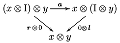
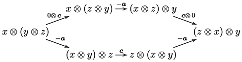
(the braidings), such that the four coherence conditions below hold.
a x , y , z t + a x y , z , t = ( 0 x a y , z , t ) + a x , y z , t + ( a x , y , z 0 t ) ,
Mathematics 03 01001 i004
( 0 x l y ) + a x , I , y = r x 0 y ,
Mathematics 03 01001 i005
( 0 y c x , z ) + a y , x , z + ( c x , y 0 z ) = a y , z , x + c x , y z + a x , y , z ,
Mathematics 03 01001 i006
( c x , z 0 y ) a x , z , y + ( 0 x c y , z ) = a z , x , y + c x y , z a x , y , z .
Mathematics 03 01001 i007
For further use, we recall that in any braided abelian ⊗-groupoid M , the equalities below hold (see [19]).
l x y + a I , x , y = l x 0 y , 0 x r y + a x , y , I = r x y ,
l x + c x , I = r x , r x + c I , x = l x .
Example 4.1 (Two-dimensional crossed products). Every commutative three-cocycle ( h , μ ) Z c 3 ( M , A ) gives rise to a braided abelian ⊗-groupoid
A h , μ M = ( A h , μ M , , I , a , l , r , c ) ,
that should be thought of as a two-dimensional crossed product of M by A , and it is built as follows: its underlying groupoid is the totally disconnected groupoid
A h , μ M = a M K ( A a , 1 ) ,
where recall that each K ( A a , 1 ) denotes the groupoid having a as its unique object and A a as the automorphism group of a. That is, an object of A h , μ M is an element a M ; if a b are different elements of the monoid M, then there are no morphisms in A h , μ M between them, whereas its isotropy group at any a M is A a .
The tensor product : ( A h , μ M ) × ( A h , μ M ) A h , μ M is given by multiplication in M on objects, so a b = a b , and on morphisms by the group homomorphisms
: A a × A b A a b , u a u b = b * u a + a * u b .
The unit object is I = 1 , the unit of the monoid M, and the structure constraints and the braiding isomorphisms are
a a , b , c = h ( a , b , c ) : ( a b ) c a ( b c ) , c a , b = μ ( a , b ) : a b b a , l a = 0 a : 1 a = a a , r a = 0 a : a 1 = a a ,
which are easily seen to be natural since A is an abelian group valued functor. The coherence condition (18), (20) and (21) follow from the three-cocycle condition 3 ( h , μ ) = ( 0 , 0 , 0 ) , while the coherence condition (19) holds due to the normalization condition h ( a , 1 , b ) = 0 .
Example 4.2. A braided abelian ⊗-groupoid is called strict if all of its structure constraints a x , y , z , l x and r x are identities. Regarding a monoid as a category with only one object, it is easy to identify a braided abelian strict ⊗-groupoid with an abelian track monoid, in the sense of Baues-Jibladze [28] and Pirashvili [29], endowed with a braided structure. Porter [30] and Joyal-Street [31] (§3, Example 4) (a preliminary manuscript of [19])) show a natural way to produce braided strict abelian ⊗-groupoids from crossed modules in the category of monoids. We recall that construction in this example.
A crossed module in the category Mon is a triplet ( G , M , ) consisting of a monoid M, a group G endowed with a M-action by a monoid homomorphism M End ( G ) , written ( a , g ) g a , and a homomorphism : G M satisfying
( g a ) a = a g , g g g = g g .
Roughly speaking, these two conditions say that the action of M on G behaves like an abstract conjugation. Note that when the monoid M is a group, we have the ordinary notion of a crossed module by Whitehead [32]. Observe that, if g = 1 , then g g = g g for all g G ; that is, the subgroup { g g = 1 } is contained in the center of G, and therefore, it is abelian. The crossed module is termed abelian whenever, for any a M , the subgroup { g g a = a } G is abelian. If, for example, the group G is abelian, or the monoid M is cancellative (a group, for instance), then the crossed module is abelian.
A bracket operation for a crossed module ( G , M , ) is a function { , } : M × M G satisfying
{ a , b } b a = a b , { 1 , b } = 1 = { a , 1 } , { g , a } g a = g , { a , g } g = g a ,
{ a b , c } = { b , c } a { a , c } , { a , b c } = { a , b } { a , c } a .
This operation should be thought of as an abstract commutator.
Each abelian crossed module with a bracket operator yields a braided abelian strict ⊗-groupoid M = M ( G , M , , { , } ) as follows. Its objects are the elements of the monoid M, and a morphism g : a b in M is an element g G with a = g b . The composition of two morphisms a g b h c is given by multiplication in G, a g h c . The tensor product is
( a g b ) ( c h d ) = ( a c g h b b d ) ,
and the braiding is provided by the bracket operator via the formula
c a , b = { a , b } : a b b a .
In the very special case where M and G are commutative, the action of M on G is trivial, and is the trivial homomorphism (i.e., g a = g and g = 1 , for all a M , g G ), then a bracket operator { , } : M × M G amounts a bilinear map, that is, a function satisfying
{ 1 , b } = 1 = { a , 1 } , { a b , c } = { a , c } { b , c } , { a , b c } = { a , b } { a , c } .
Thus, for example, when M = N is the additive monoid of non-negative integers and G = Z is the abelian group of integers, a bracket N × N Z is given by { p , q } = p q . Furthermore, if G is any multiplicative abelian group, then any g G defines a bracket N × N G by { p , q } = g p q .
Suppose M , M 
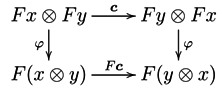
are braided abelian ⊗-groupoids. A braided ⊗-functor (or braided monoidal functor)
F = ( F , φ , φ 0 ) : M M
consists of a functor on the underlying groupoids F : M M , natural isomorphisms φ x , y : F x F y F ( x y ) and an isomorphism φ 0 : I F I , such that the following coherence conditions hold
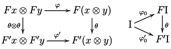
F a x , y , z + φ x y , z + ( φ x , y 0 F z ) = φ x , y z + ( 0 F x φ y , z ) + a F x , F y , F z ,
Mathematics 03 01001 i008
F l x + φ I , x + ( φ 0 0 F x ) = l F x , F r x + φ x , I + ( 0 F x φ 0 ) = r F x ,
Mathematics 03 01001 i009
φ y , x + c F x , F y = F c x , y + φ x , y .
Mathematics 03 01001 i010
If F : M M is another braided ⊗-functor, then an isomorphism θ : F F is a natural isomorphism on the underlying functors, θ : F F , such that the coherence conditions below are satisfied.
θ x y + φ x , y = φ x , y + ( θ x θ y ) , θ I + φ 0 = φ 0 .
Mathematics 03 01001 i011
Example 4.3. Let ( h , μ ) , ( h , μ ) Z c 3 ( M , A ) be commutative three-cocycles of a commutative monoid. Then, any commutative cochain g C c 2 ( M , A ) , such that ( h , μ ) = ( h , μ ) + 2 g induces a braided ⊗-isomorphism
F ( g ) = ( i d , g , 0 1 ) : A h , μ M A h , μ M
which is the identity functor on the underlying groupoids and whose structure isomorphisms are given by φ a , b = g ( a , b ) : a b a b and φ 0 = 0 1 : 1 1 , respectively. Since the groups A a b are abelian, these isomorphisms φ a , b are natural. The coherence condition (26) and (28) follow from the equality ( h , μ ) = ( h , μ ) + 2 g , whilst the conditions in (27) trivially hold because of the normalization conditions g ( a , 1 ) = 0 a = g ( 1 , a ) .
If f C c 1 ( M , A ) is any commutative one-cochain and g = g + 1 f C c 2 ( M , A ) , then an isomorphism of braided ⊗-functors θ ( f ) : F ( g ) F ( g ) is defined by putting θ ( f ) a = f ( a ) : a a , for each a M . So defined, θ is natural because of the abelian structure of the groups A a ; the first condition in (29) holds owing to the equality g = g + 1 f and the second one thanks to the normalization condition f ( 1 ) = 0 1 of f.
With compositions defined in a natural way, braided abelian ⊗-groupoids, braided ⊗-functors and isomorphisms form a 2-category [16] (Chapter V, §1). A braided ⊗-functor F : M M is called a braided ⊗-equivalence if it is an equivalence in this 2-category of braided abelian ⊗-groupoids, that is when there exists a braided ⊗-functor F : M M and braided isomorphisms η : i d M F F and ε : F F i d M . From [4] (I, Proposition 4.4.2), it follows that a braided ⊗-functor F : M M is a braided ⊗-equivalence if and only if the underlying functor is an equivalence of groupoids, that is if and only if it is full, faithful and essentially surjective on objects or [33] (Chapter 6, Corollary 2) if and only if the induced map on the sets of iso-classes of objects
Ob M / Ob M / , [ x ] [ F x ] ,
is a bijection, and the induced homomorphisms on the automorphism groups
Aut M ( x ) Aut M ( F x ) , u F u ,
are all isomorphisms.
Remark 4.4. From the coherence theorem for monoidal categories [19] (Corollary 1.4, Example 2.4), it follows that every braided abelian ⊗-groupoid is braided ⊗-equivalent to a braided strict one, that is to one in which all of the structure constraints a x , y , z , l x and r x are identities (see Example 4.2). This suggests that it is relatively harmless to consider braided abelian ⊗-groupoids as strict. However, it is not so harmless when dealing with their homomorphisms, since not every braided ⊗-functor is isomorphic to a strict one (i.e., one as in (25) in which the structure isomorphisms φ x , y and φ 0 are all identities). Indeed, it is possible to find two braided abelian strict ⊗-groupoids, say M and M , that are related by a braided ⊗-equivalence between them, but there is no strict ⊗-equivalence either from M to M nor from M to M .
Our goal is to state a classification for braided abelian ⊗-groupoids, where two of them connected by a braided ⊗-equivalence are considered the same. The main result in this section is the following
Theorem 4.5 (Classification of braided abelian ⊗-groupoids). ( i ) For any braided abelian ⊗-groupoid M , there exist a commutative monoid M, a functor A : H M Ab , a commutative three-cocycle ( h , μ ) Z c 3 ( M , A ) and a braided ⊗-equivalence
A h , μ M M .
( i i ) For any two commutative three-cocycles ( h , μ ) Z c 3 ( M , A ) and ( h , μ ) Z c 3 ( M , A ) , there is a braided ⊗-equivalence:
A h , μ M A h , μ M
if and and only if there exist an isomorphism of monoids i : M M and a natural isomorphism ψ : A A i , such that the equality of cohomology classes below holds.
[ h , μ ] = ψ * 1 i * [ h , μ ] H c 3 ( M , A )
Proof. ( i ) Let M = ( M , , I , a , l , r , c ) be any given braided abelian ⊗-groupoid.
In a first step, we assume that M is totally disconnected and strictly unitary, in the sense that its unit constraints l x and r x are all identities. Then, a system of data ( M , A , ( h , μ ) ) , such that A h , μ M = M as braided abelian groupoids, is defined as follows:
• The monoid M. Let M = Ob M be the set of objects of M . The function on objects of the tensor functor : M × M M determines a multiplication on M, simply by making a b = a b , for any a , b M . Because of the strictness of the unit in M , this multiplication on M is unitary with 1 = I , the unit object of M . Furthermore, it is associative and commutative since, as M is totally disconnected, the existence of the associativity constraints ( a b ) c a ( b c ) and the braidings a b b a forces the equalities ( a b ) c = a ( b c ) and a b = b a . Thus, M becomes a commutative monoid.
• The functor A : H M Ab . For each a M = Ob M , let A a = Aut M ( a ) be the vertex group of the underlying groupoid at a. The group homomorphisms : A a × A b A a b have an associative, commutative and unitary behavior in the sense that the equalities
( u a u b ) u c = u a ( u b u c ) , u a u b = u b u a , 0 1 u a = u a ,
hold. These follow from the abelian nature of the groups of automorphisms in M , since the diagrams below commute due to the naturality of the structure constraints and the braiding.
Mathematics 03 01001 i012
Then, if we write b * : A a A a b for the homomorphism, such that
b * u a : = 0 b u a = u a 0 b ,
the equalities:
( b c ) * ( u a ) = 0 b c u a = ( 0 b 0 c ) u a = ( 31 ) 0 b ( 0 c u a ) = b * ( c * u a ) , 1 * u a = 0 1 u a = ( 31 ) u a ,
show that the assignments a A a , ( a , b ) b * : A a A a b , define an abelian group valued functor on H M . Note that this functor determines the tensor product ⊗ of M , since
u a u b = ( u a + 0 a ) ( 0 b + u b ) = ( u a 0 b ) + ( 0 a u b ) = ( 31 ) ( 0 b u a ) + ( 0 a u b ) = b * u a + a * u b .
• The three-cocycle ( h , μ ) Z c 3 ( M , A ) . The associativity constraint and the braiding of M are necessarily written in the form a a , b , c = h ( a , b , c ) and c a , b = μ ( a , b ) , for some given lists h ( a , b , c ) A a b c a , b , c M and μ ( a , b ) A a b a , b M . Since M is strictly unitary, the equations in (19) and (22) give the normalization conditions h ( a , 1 , b ) = 0 = h ( 1 , a , b ) = h ( a , b , 1 ) for h, while the equations in (23) imply the normalization conditions μ ( a , 1 ) = 0 = μ ( 1 , a ) for μ. Thus, ( h , μ ) C c 3 ( M , A ) is a commutative three-cochain, which is actually a three-cocycle, since the coherence conditions (18), (20) and (21) are now written as
h ( a , b , c d ) + h ( a b , c , d ) = a * h ( b , c , d ) + h ( a , b c , d ) + d * h ( a , b , c ) b * μ ( a , c ) + h ( b , a , c ) + c * μ ( a , b ) = h ( b , c , a ) + μ ( a , b c ) + h ( a , b , c ) , b * μ ( a , c ) h ( a , c , b ) + a * μ ( b , c ) = h ( c , a , b ) + μ ( a b , c ) h ( a , b , c ) ,
which amount to the cocycle condition 3 ( h , μ ) = ( 0 , 0 , 0 ) .
Since an easy comparison (see Example 4.1) shows that M = A h , μ M , the proof of this part is complete, under the hypothesis of being M totally disconnected and strictly unitary.
It remains to prove that the braided abelian ⊗-groupoid M is braided ⊗-equivalent to another one M that is totally disconnected and strictly unitary. To do that, we combine the transport process by Saavedra [4] (I, 4.4.5) and Joyal-Street [19] (Example 2.4), which shows how to transport the braided monoidal structure on an abelian ⊗-groupoid along an equivalence on its underlying groupoid, with the generalized Brandt’s theorem, which asserts that every groupoid is equivalent (as a category) to a totally disconnected groupoid [33] (Chapter 6, Theorem 2). Since every braided abelian ⊗-groupoid is braided ⊗-equivalent to a braided abelian strict ⊗-groupoid (see Remark 4.4), there is no loss of generality in assuming that M is itself strictly unitary.
Then, let M = Ob M / be the set of isomorphism classes [ x ] of the objects of M ; let us choose, for each a M , any representative object x a a , with x [ I ] = I ; and let us form the totally disconnected abelian groupoid
M = a M K ( A a , 1 ) ,
whose set of objects is M and whose vertex group at any object a M is A a = Aut M ( x a ) .
This groupoid M is equivalent to the underlying groupoid M . To give a particular equivalence F : M M , let us select for each a M and each x a an isomorphism η x : x x a in M . In particular, for every a M , we take η x a = 0 x a , the identity morphism of x a . Then, let F : M M be the functor that acts on objects by F x = [ x ] and on morphisms u : x y by F u = η y + u η x . We also have the more obvious functor F : M M , which is defined on objects by F a = x a and on morphisms u : a a by F u = u . Clearly, F F = i d M , and the natural equivalence η : i d M F F satisfies the equalities F η = i d F and η F = i d F . Therefore, the given braided monoidal structure on M can be transported to one on M , such that the functors F and F underlie braided ⊗-functors, and the natural equivalences η : i d M F F and i d : F F i d M 
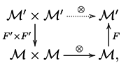
turn out to be ⊗-isomorphisms. In the transported structure, the tensor product : M × M M is the dotted functor in the commutative square
Mathematics 03 01001 i013
and the unit object is F I = [ I ] . The functors F and F are endowed with the isomorphisms
φ x , y = F ( η x η y ) : F x F y F ( x y ) , φ 0 = 0 [ I ] : [ I ] F I = [ I ] , φ a , b = η x a x b : F a F b F ( a b ) , φ 0 = 0 I : I F [ I ] = I ,
and the structure constraints a , r , l and the braiding c of M are those isomorphisms uniquely determined by (26)–(28), respectively. Now, a quick analysis indicates that, for any object a Ob M = M ,
r a = ( 27 ) F ( r x a ) + φ x a , I + ( 0 a φ 0 ) = φ x a , I = F ( η x a η I ) = F ( 0 x a 0 I ) = F ( 0 x a I ) = F ( 0 x a ) = 0 a
Similarly, we have l a = 0 a , and therefore, M is strictly unitary.
( i i ) We first assume that there exist an isomorphism of monoids i : M M and a natural isomorphism ψ : A A i , such that ψ * [ h , μ ] = i * [ h , μ ] H c 3 ( M , A i ) . This means that there is a commutative two-cochain g C c 2 M , A i ) , such that the equalities below hold.
ψ a b c h ( a , b , c ) = h ( i a , i b , i c ) + ( i a ) * g ( b , c ) g ( a b , c ) + g ( a , b c ) ( i c ) * g ( a , b ) ,
ψ a b μ ( a , b ) = μ ( i a , i b ) g ( a , b ) + g ( b , a ) .
Then, a braided isomorphism:
F ( g ) = ( F , φ , φ 0 ) : A h , μ M A h , μ M
is defined as follows. The underlying functor acts by F ( u a : a a ) = ( ψ a ( u a ) : i a i a ) . The structure isomorphisms of F are given by φ a , b = g ( a , b ) : ( i a ) ( i b ) i ( a b ) and φ 0 = 0 1 : 1 i 1 = 1 . So defined, it is easy to see that F is an isomorphism between the underlying groupoids. Verifying the naturality of the isomorphisms φ a , b , that is the commutativity of the squares
Mathematics 03 01001 i014
for u a A a , u b A b , is equivalent (since the groups A i ( a b ) are abelian) to verify the equalities
ψ a b ( a * u b + b * u a ) = ( i a ) * ψ b u b + ( i b ) * ψ a u a ,
which hold since the naturality of ψ : A A i just says that
ψ a b ( a * u b ) = ( i a ) * ψ b u b .
The coherence conditions (26) and (28) are verified as follows
φ a , b c + ( 0 F a φ b , c ) + a F a , F b , F c = φ a , b c + ( i a ) * φ b , c + h ( i a , i b , i c ) = g ( a , b c ) + ( i a ) * g ( b , c ) + h ( i a , i b , i c ) = ( 32 ) ψ a b c h ( a , b , c ) + g ( a b , c ) + ( i c ) * g ( a , b ) = ψ a b c h ( a , b , c ) + φ a b , c + ( i c ) * φ a , b = F ( a a , b , c ) + φ a b , c + ( φ a , b 0 F c ) ,
φ b , a + c F a , F b = g ( b , a ) + μ ( i a , i b ) = ( 33 ) ψ a b ( μ ( a , b ) ) + g ( a , b ) = F ( c a , b ) + φ a , b ,
whereas the conditions in (27) trivially follow from the equalities g ( a , 1 ) = 0 i a = g ( 1 , a ) .
Conversely, suppose that F = ( F , φ , φ 0 ) : A h , μ M A h , μ M is any braided equivalence. By [18], there is no loss of generality in assuming that F is strictly unitary in the sense that φ 0 = 0 1 : 1 1 = F 1 . As the underlying functor establishes an equivalence between the underlying groupoids,
F : a M K ( A a , 1 ) a M K ( A a , 1 ) ,
and these are totally disconnected, it is necessarily an isomorphism.
Let us write i : M M for the bijection describing the action of F on objects; that is, such that i a = F a , for each a M . Then, i is actually an isomorphism of monoids, since the existence of the structure isomorphisms φ a , b : ( i a ) ( i b ) i ( a b ) forces the equality ( i a ) ( i b ) = i ( a b ) .
Let us write ψ a : A a A i a for the isomorphism giving the action of F on automorphisms u a : a a ; that is, such that F u a = ψ a u a , for each u a A a and a M . The naturality of the automorphisms φ a , b tell us that the equalities (36) hold (see diagram (35)). These, for the case when u a = 0 a , give the equalities in (37), which amounts to ψ : A A i being a natural isomorphism of abelian group valued functors on H M .
Writing now g ( a , b ) = φ a , b , for each a , b M , the equations g ( a , 1 ) = 0 i a = g ( 1 , a ) hold due to the coherence (27), and thus, we have a commutative two-cochain
g ( F ) = g ( a , b ) A i ( a b ) a , b M ,
which satisfies (32) and (33) owing to the coherence (26) and (28), as we can see just by retracting our steps in (38) and (39), respectively. This means that ψ * ( h , μ ) = i * ( h , μ ) 2 g , and therefore, we have that ψ * [ h , μ ] = i * [ h , μ ] H c 3 ( M , A i ) , whence [ h , μ ] = ψ * 1 i * [ h , μ ] H c 3 ( M , A ) . □
A braided categorical group [19] (§3) is a braided abelian ⊗-groupoid G = ( G , , I , a , l , r , c ) in which, for any object x, there is an object x * with an arrow x x * I . Actually, the hypothesis of being abelian is superfluous here, since every monoidal groupoid in which every object has a quasi-inverse is always abelian [2] (Proposition 3). The cohomological classification of these braided categorical groups was stated and proven by Joyal and Street [19] (Theorem 3.3) by means of Eilenberg–Mac Lane’s commutative cohomology groups H c 3 ( G , A ) , of abelian groups G with coefficients in abelian groups A (see Example 3.2). Next, we obtain Joyal–Street’s classification result as a corollary of Theorem 4.5.
Corollary 4.6. ( i ) For any abelian groups G and A and any three-cocycle ( h , μ ) Z c 3 ( G , A ) , the braided abelian groupoid A h , μ G is a braided categorical group.
( i i ) For any braided categorical group G , there exist abelian groups G and A, a three-cocycle ( h , μ ) Z c 3 ( G , A ) and a braided ⊗-equivalence
A h , μ G G .
( i i i ) For any two commutative three-cocycles ( h , μ ) Z c 3 ( G , A ) and ( h , μ ) Z c 3 ( G , A ) , where G , G , A and A are abelian groups, there is a braided ⊗-equivalence
A h , μ G A h , μ G
if and and only if there exist isomorphism of groups i : G G and ϕ : A A , such that the equality of cohomology classes below holds.
[ h , μ ] = ϕ * i * [ h , μ ] H c 3 ( G , A )
Proof. ( i ) Recall from Example 3.2 that we are here regarding A as the constant abelian group valued functor on H G it defines. Since G is a group, for any object a of A h , μ G (i.e., any element a G ), we have a a 1 = a a 1 = 1 = I . Thus, A h , μ G is actually a braided categorical group.
( i i ) Let G be a braided categorical group. By Theorem 4.5 ( i ) , there are a commutative monoid M, a functor A : H M Ab , a commutative three-cocycle ( h , μ ) Z c 3 ( M , A ) and a braided ⊗-equivalence A h , μ M G . Then, A h , μ M is a braided categorical group as G is, and for any a M , it must exist another a * M with a morphism a a * = a a * I = 1 in A h , μ M ; this implies that a a * = 1 in M, since the groupoid is totally disconnected, whence a * = a 1 is an inverse of a in M. Therefore, M = G is actually an abelian group.
Let A 1 be the abelian group attached by A at the unit of G. Then, a natural isomorphism ϕ : A A 1 is defined, such that, for any a G , ϕ a = a * 1 : A a A 1 . Therefore, if we take ( h , μ ) = ϕ * ( h , μ ) Z c 3 ( G , A 1 ) , Theorem 4.5 ( i i ) gives the existence of a braided equivalence A h , μ G A 1 h , μ G , whence A 1 h , μ G , and the given G are braided ⊗-equivalent.
( i i i ) This follows directly form Theorem 4.5 ( i i ) . □
The classification result in Theorem 4.5 involves an interpretation of the elements of H c 3 ( M , A ) in terms of certain two-dimensional co-extensions of M by A , such as the elements of H c 2 ( M , A ) are interpreted as commutative monoid co-extensions in Corollary 3.8. To state this fact, in the next definition, we regard any commutative monoid M as a braided abelian discrete ⊗-groupoid (i.e., whose only morphisms are the identities), on which the tensor product is multiplication in M. Thus, if M = ( M , , I , a , l , r , c ) is any braided abelian ⊗-groupoid, a braided ⊗-functor p : M M is the same thing as a map p : Ob M M satisfying p ( x ) = p ( y ) whenever Hom M ( x , y ) , p ( x y ) = p ( x ) p ( y ) and p ( I ) = 1 .
Definition 4.7. Let M be a commutative monoid, and let A be any abelian group valued functor on H M . A braided two-coextension of M by A is a surjective braided ⊗-functor p : M M , where M is a braided abelian ⊗-groupoid, such that, for any a M , it is given an (associative and unitary) action of the groupoid K ( A a , 1 ) on the fiber groupoid p 1 ( a ) by means of a functor
K ( A a , 1 ) × p 1 ( a ) p 1 ( a ) , ( u , x f y ) ( x u · f y )
which is simply transitive, in the sense that the induced functor:
K ( A a , 1 ) × p 1 ( a ) p 1 ( a ) × p 1 ( a ) , ( u , f ) ( u · f , f ) ,
is an equivalence and satisfies
( u · f ) ( v · g ) = ( a * v + b * u ) · ( f g ) ,
for every a , b M , u A a , v A b , f : x y p 1 ( a ) and g : z t p 1 ( b ) .
Let us point out that if p ( x ) = p ( y ) , for some x , y Ob M , then Hom M ( x , y ) since the functor K ( A a , 1 ) × p 1 ( a ) p 1 ( a ) , for a = p ( x ) , is essentially surjective. Furthermore, the functoriality of the action means that if f , f are composablearrows in p 1 ( a ) , then, for any u , u A a , we have
( u + u ) · ( f + f ) = u · f + u · f .
In particular,
f + u · f = u · ( f + f ) = u · f + f .
Remark 4.8. These braided two-co-extensions can be seen as a sort of (braided, non-strict) linear track extensions in the sense of Baues, Dreckmann and Jibladze [28,34]. Briefly, note that to give a commutative two-coextension p : M M , as above, is equivalent to giving a surjective braided ⊗-functor p : M M satisfying
p ( x ) = p ( y ) if and only if Hom M ( x , y ) ,
together with a family of isomorphisms of groups ψ x : A p x Aut M ( x ) x Ob M satisfying:
ψ y u = f + ψ x u f , f Hom M ( x , y ) , ψ x u ψ y v = ψ x y ( ( p x ) * v + ( p y ) * u ) , x , y Ob M .
The family of isomorphisms ( ψ x ) x Ob M and the action of A on M are related to each other by the equations u · f = f + ψ x ( u ) , for any x Ob M , u A p ( x ) , and f Hom M ( x , y ) .
Let Ext c 2 ( M , A ) denote the set of equivalence classes of such braided two-co-extensions of M by A , where two of them, say p : M M and p : M M , are equivalent whenever there is a braided ⊗-equivalence F : M M , such that p F = p and F ( u · f ) = u · F ( f ) , for any morphism f : x y in M and u A p ( x ) . Then, we have:
Theorem 4.9 (Classification of braided two-co-extensions). For any commutative monoid M and any functor A : H M Ab , there is a natural bijection
H c 3 ( M , A ) Ext c 2 ( M , A ) .
Proof. This is a consequence of Theorem 4.5 with only a slight adaptation of the arguments used for its proof. For any three-cocycle ( h , μ ) Z c 3 ( M , A ) , the braided abelian ⊗-groupoid A h , μ M in (24) comes with a natural structure of braided two-coextension of M by A , in which the surjective braided functor π : A h , μ M M is given by the identity map on objects, π ( a ) = a . The fiber groupoid over any a M is just π 1 ( a ) = K ( A a , 1 ) , and the action functor K ( A a , 1 ) × π 1 ( a ) π 1 ( a ) is given by addition in A a , that is u · v = u + v . If ( h , μ ) Z c 3 ( M , A ) in any other three-cocycle, such that ( h , μ ) = ( h , μ ) 2 g , for some two-cochain g C c 2 ( M , A ) , then the associated braided ⊗-isomorphism in (30), F ( g ) : A h , μ M A h , μ M , is easily recognized as an equivalence between the braided co-extensions A h , μ M M and A h , μ M M . Thus, we have a well-defined map
H c 3 ( M , A ) Ext c 2 ( M , A ) , [ h , μ ] [ A h , μ M π M ] .
To see that it is injective, suppose ( h , μ ) , ( h , μ ) Z c 3 ( M , A ) , such that the associated braided two-co-extensions are made equivalent by a braided ⊗-functor, say F : A h , μ M A h , μ M , which can be assumed to be strictly unitary [18]. Then, the two-cochain g ( F ) C c 2 ( M , A ) built in (40) satisfies that ( h , μ ) = ( h , μ ) 2 g , whence [ h , μ ] = [ h , μ ] H c 3 ( M , A ) .
Finally, to prove that the map is surjective, let p : M M be any given braided two-coextension of M by A . By Theorem 4.5 ( i ) and Lemma 4.10 below, we can assume that M = A h , μ M , for some commutative monoid M , a functor A : H M Ab , and a three-cocycle ( h , μ ) Z c 3 ( M , A ) . Then, a monoid isomorphism i : M M and a natural isomorphism ψ : A A i become determined by the equations p ( i a ) = a and ψ a ( u ) = u · 0 i a , for any a M and u A a . Furthermore, taking ( h , μ ) = ψ * 1 i * ( h , μ ) Z c 3 ( M , A ) , the braided ⊗-isomorphism in (34) for the two-cochain g = 0 , F ( 0 ) : A h , μ M A h , μ M , is then easily seen as an equivalence between the braided extensions π : A h , μ M M and p : M M . □
Lemma 4.10. Let p : M M be a braided two-coextension of M by A , and suppose that M is any braided abelian ⊗-groupoid, which is braided ⊗-equivalent to M . Then, M can be endowed with a braided two-coextension structure of M by A , say p : M M , such that p : M M and p : M M are equivalent braided two-co-extensions. □
Proof. Let F = ( F , φ ) : M M be a braided ⊗-equivalence. Then, a braided two-coextension structure of M is given as follows: let:
p = p F : M M
be the braided ⊗-functor composite of p and F. This is clearly surjective, since p is and F is essentially surjective. For every a M , let K ( A a , 1 ) × p 1 ( a ) p 1 ( a ) be the action defined by ( u , x f y ) ( x u · f y ) , where u · f is unique arrow in M , such that
F ( u · f ) = u · F f .
This is a simply-transitive well-defined action since F is a full, faithful and essentially surjective functor. In order to check (41), we have:
F ( ( u · f ) ( v · g ) ) + φ x z = φ y t + F ( u · f ) F ( v · g ) ( nat . of φ ) = φ y t + ( u · F f ) ( v · F g ) ( 43 ) = φ y t + ( a * u + b * v ) · ( F f F g ) ( ( 41 ) for M M ) = ( a * v + b * v ) · F ( f g ) + φ x z ( nat . of φ and ( 42 ) ) = F ( ( a * v + b * u ) · ( f g ) ) + φ x z ( 43 )
and the result follows since F is faithful and φ x z is an isomorphism. Thus, we have defined the braided two-coextension M M , which is clearly equivalent to the original one by means of F. □

Acknowledgments

This work has been supported by “Dirección General de Investigación” of Spain, Project: MTM2011-22554; and for the first author also by FPUgrant FPU12-01112.

Author Contributions

Both authors have contributed equally to this work and they agree to the final version.

Conflicts of Interest

The authors declare no conflict of interest.

References

  1. Leech, J. Two papers: -co-extensions of monoids and the structure of a band of groups; Memoirs Amer Mathematical Society: Providence, RL, USA, 1975; Volume 157. [Google Scholar]
  2. Calvo-Cervera, M.; Cegarra, A.M.; Heredia, B.A. Structure and classification of monoidal groupoids. Semigr. Forum 2013, 87, 35–79. [Google Scholar] [CrossRef]
  3. Mac Lane, S. Natural associativity and commutativity. Rice Univ. Stud. 1963, 49, 28–46. [Google Scholar]
  4. Saavedra, N. Catégories Tannakiennes; Springer-Verlag: Berlin, Germany, 1972; Volume 265. [Google Scholar]
  5. Grillet, P.A. Commutative semigroup cohomology. Semigr. Forum 1991, 43, 247–252. [Google Scholar] [CrossRef]
  6. Grillet, P.A. Commutative semigroup cohomology. Commun. Algebra 1995, 23, 3573–3587. [Google Scholar] [CrossRef]
  7. Grillet, P.A. Cocycles in commutative semigroup cohomology. Commun. Algebra 1997, 25, 3427–3462. [Google Scholar] [CrossRef]
  8. Grillet, P.A. Commutative Semigroups; Springer Science & Business Media: New York, NY, USA, 2001. [Google Scholar]
  9. Calvo-Cervera, M.; Cegarra, A.M.; Heredia, B.A. On the third cohomology group of a commutative monoid. Semigr. Forum 2015. [Google Scholar] [CrossRef]
  10. Deligne, P. La Formule de Dualité Globale, Exposé XVIII of Théorie de Topos et Cohomologie Etale des Schémas (SGA 4); Springer-Verlag: Berlin, Germany, 1973. [Google Scholar]
  11. Fröhlich, A.; Wall, C.T. Graded monoidal categories. Compos. Math. 1974, 28, 229–285. [Google Scholar]
  12. Eilenberg, S.; Mac Lane, S. Cohomology theory of abelian groups and homotopy theory, I. Proc. Nat. Acad. Sci. USA 1950, 36, 443–447. [Google Scholar] [CrossRef] [PubMed]
  13. Eilenberg, S.; Mac Lane, S. Cohomology theory of abelian groups and homotopy theory, II. Proc. Nat. Acad. Sci. USA 1950, 36, 657–663. [Google Scholar] [CrossRef] [PubMed]
  14. Eilenberg, S.; Mac Lane, S. Cohomology theory of abelian groups and homotopy theory, III. Proc. Nat. Acad. Sci. USA 1951, 37, 307–310. [Google Scholar] [CrossRef] [PubMed]
  15. Mac Lane, S. Cohomology theory of abelian groups. Proc. Int. Cong. Math. 1950, 2, 8–14. [Google Scholar]
  16. Gabriel, P.; Zisman, M. Calculus of Fractions and Homotopy Theory; Springer: Berlin, Germany, 1967. [Google Scholar]
  17. Eilenberg, S.; Mac Lane, S. On the groups H(π,n), I. Ann. Math. 1953, 58, 55–106. [Google Scholar] [CrossRef]
  18. Cegarra, A.M.M.; Khadmaladze, E. Homotopy classification of braided graded categorical groups. J. Pure Appl. Algebra 2007, 209, 411–437. [Google Scholar] [CrossRef]
  19. Joyal, A.; Street, R. Braided tensor categories. Adv. Math. 1991, 82, 20–78. [Google Scholar] [CrossRef]
  20. Mac Lane, S. Categories for the Working Mathematician; Springer Science & Business Media: New York, NY, USA, 1971. [Google Scholar]
  21. Barr, M.; Beck, J. Homology and standard constructions. In Seminar on Triples and Categorical Homology; Springer: Berlin, Geramny, 1969. [Google Scholar]
  22. Roos, J.E. Sur les foncteurs dérivés de projlim. Applications. C. R. Acad. Sci. Paris 1961, 252, 3702–3704. [Google Scholar]
  23. Wells, C. Extension theories for monoids. Semigr. Forum 1978, 16, 13–35. [Google Scholar] [CrossRef]
  24. May, J.P. Simplicial Objects in Algebraic Topology; Van Nostrand Reinhold: Princeton, NJ, USA, 1967. [Google Scholar]
  25. Calvo-Cervera, M.; Cegarra, A.M.; Quang, N.T. Higher cohomologies of modules. Algebraic Geomet. Topol. 2012, 12, 343–413. [Google Scholar] [CrossRef]
  26. Eilenberg, S.; Mac Lane, S. On the groups H(π,n), II. Ann. Math. 1954, 70, 49–137. [Google Scholar] [CrossRef]
  27. Goerss, P.G.; Jardine, J.F. Simplicial Homotopy Theory; Birkhauser: Boston, MA, USA; Basel, Switzerland; Berlin, Geramny, 1999; Volume 174. [Google Scholar]
  28. Baues, H.-J.; Jibladze, M. Classification of Abelian Track Categories. K-Theory 2002, 25, 299–311. [Google Scholar] [CrossRef]
  29. Pirashvili, T. Groupoid enriched categories and natural systems. Theory Appl. Categ. 2005, 14, 286–293. [Google Scholar]
  30. Porter, T. Crossed modules in Cat and Brown-Spencer theorem for 2-categories. Cahiers Topol. Géom. Differ. Catég. 1985, 26, 381–388. [Google Scholar]
  31. Joyal, A.; Street, R. Braided Monoidal Categories; Macquarie Mathematics Reports; Macquarie University: Syndey, Australia, 1986. [Google Scholar]
  32. Whitehead, J.H.C. Combinatorial homotopy II. Bull. Am. Math. Soc. 1999, 55, 496–543. [Google Scholar] [CrossRef]
  33. Higgings, P.J. Categories and groupoids. Reprints Theory Appl. Categ. 2005, 7, 1–195. [Google Scholar]
  34. Baues, H.-J.; Dreckmann, W. The cohomology of homotopy categories and the general linear group. K-Theory 1989, 3, 307–338. [Google Scholar] [CrossRef]

