Twistor Interpretation of Harmonic Spheres and Yang–Mills Fields

Abstract

We consider the twistor descriptions of harmonic maps of the Riemann sphere into Kähler manifolds and Yang–Mills fields on four-dimensional Euclidean space. The motivation to study twistor interpretations of these objects comes from the harmonic spheres conjecture stating the existence of the bijective correspondence between based harmonic spheres in the loop space ΩG of a compact Lie group G and the moduli space of Yang–Mills G-fields on ℝ⁴.

1. Introduction

In the first part of this paper, we consider the twistor interpretation of harmonic maps of the Riemann sphere into Kähler manifolds.

Harmonic maps of the Riemann sphere S := ℙ¹ into a given Riemannian manifold M (harmonic spheres) are the extrema of the energy functional, given by the Dirichlet-type integral. If M is Kähler, then holomorphic and anti-holomorphic spheres are local minima of the energy. However, for dim_ℂ M > 1, this functional usually has non-minimal critical points. For any even-dimensional Riemannian manifold M, we can construct a twistor bundle π : Z → M over M, where Z is an almost complex manifold having the following property: for any pseudoholomorphic sphere ψ : S → Z, its projection φ := π ○ ψ to M is a harmonic sphere φ : S → M. Moreover, in the case when M coincides with the Grassmann manifold Gr_r (ℂⁿ), any harmonic sphere in this manifold can be obtained in this way. These results may be extended to infinite-dimensional Kähler manifolds M (cf. [1]). If, in particular, M coincides with the loop space ΩG of a compact Lie group, we have an infinite-dimensional analogue of the above result for the Grassmannian Gr_r(ℂⁿ). Namely, in the paper [2], we prove that any harmonic sphere in the loop space ΩG, embedded into the Hilbert–Schmidt Grassmannian Gr_HS(H), may be obtained as the projection of some pseudoholomorphic sphere in a virtual flag bundle over Gr_HS(H) (as is explained in more detail in Section 4).

In the second part of the paper, we consider the Yang–Mills fields on ℝ⁴ with gauge group G. They are the extrema of the Yang–Mills action functional. The local minima of this functional are given by instantons and anti-instantons. Their twistor description was proposed by Atiyah–Ward [3] with the help of the Hopf bundle π : ℙ³ → S⁴ over the compactified Euclidean four-space, coinciding with the sphere S⁴. In terms of this bundle, instantons correspond to the holomorphic vector bundles over ℙ³, which are trivial along the fibers of π. Using this description, Atiyah–Hitchin–Drinfeld–Manin [4] gave the complete description of the moduli space of G-instantons on ℝ⁴.

However, the structure of the moduli space of all Yang–Mills fields on ℝ⁴ is still far from being understood. The twistor description of Yang–Mills fields was proposed in the papers by Manin [5], Witten [6] and Isenberg-Green-Yasskin [7]. They are interpreted as holomorphic vector bundles over the incidence quadric in ℙ³ × (ℙ³)^∗ with some special properties described below.

We should explain now why we are interested in studying twistor interpretations of harmonic spheres in ΩG and Yang–Mills fields on ℝ⁴. The motivation comes from a theorem of Atiyah and Donaldson (cf. [8,9]) stating the existence of the bijective correspondence between the moduli space of G-instantons on ℝ⁴ and based holomorphic spheres in ΩG. A natural generalization of this theorem leads to the harmonic spheres conjecture (cf. [10]) asserting that the bijective correspondence should exist between the moduli space of Yang–Mills G-fields on R⁴ and based harmonic spheres in ΩG.

Unfortunately, the proof of the Atiyah–Donaldson theorem does not extend to the harmonic case. In our paper [11], we have proposed an approach to the proof of the harmonic spheres conjecture based on twistor methods. A key idea is to deduce this conjecture from its twistor version. This version is obtained by pulling up both objects, entering the harmonic spheres conjecture, i.e., harmonic spheres and Yang–Mills fields, to the corresponding twistor spaces. Following the general ideology of the Penrose twistor program, the twistor version of the conjecture may be proven using only holomorphic means. This motivated the study of the twistor interpretation of these objects.

We should also add that the proof of the harmonic spheres conjecture will give a new information on Yang–Mills fields, since harmonic maps are much better understood compared to their Yang–Mills counterpart. For example, one of the corollaries of this conjecture would be the existence of a Bäcklund-type procedure allowing one to construct any Yang–Mills field from a trivial one by successively adding instantons and anti-instantons.

We start by recalling basic properties of harmonic maps into Kähler manifolds in Section 1. In Section 2, we give an overview of the twistor method of the construction of harmonic maps into Kähler manifolds. This method is applied in Section 3 to the construction of harmonic spheres in complex projective spaces and Grassmannians G_r(ℂⁿ). In Section 4, we extend these results to the infinite-dimensional situation, namely to the construction of harmonic spheres in the Hilbert–Schmidt Grassmannian Gr_HS(H). The loop space ΩG can be isometrically embedded into Gr_HS(H), so that harmonic spheres φ : S → ΩG can be considered as harmonic spheres in the Grassmannian Gr_HS(H). In Section 5, we introduce the Yang–Mills fields and instantons on ℝ⁴ and give their twistor interpretation due to Atiyah and Ward. Section 6 is devoted to the Atiyah–Donaldson interpretation of instantons with gauge group G as holomorphic spheres in the loop space ΩG. We also formulate here the harmonic spheres conjecture relating Yang–Mills G-fields on ℝ⁴ with harmonic spheres in ΩG and overview the idea of its proof.

2. Harmonic Spheres in Kähler Manifolds

2.1. Complex Structures and Kähler Manifolds

Let M be a smooth manifold of dimension 2n. An almost complex structure on M is a smooth section J of the bundle End(T M), satisfying the relation J² = −I.

Denote by T^ℂM = TM ⊗_ℝ ℂ the complexified tangent bundle of the manifold M. If we fix a local basis of the bundle T^ℂM in a neighborhood of a point p ∈ M, given by the vector fields of the form:

$$\frac{\partial }{\partial z^1},\dots ,\frac{\partial }{\partial z^n},\frac{\partial }{\partial {\overline{z}}^1},\dots ,\frac{\partial }{\partial {\overline{z}}^n},$$

then any smooth complex vector field, i.e., a local section of the bundle T^ℂM in the neighborhood of p, will be written in the form:

$$X={\displaystyle \sum _j\left(X^j\frac{\partial }{\partial z^j}+X^{\overline{j}}\frac{\partial }{\partial {\overline{z}}^j}\right)}$$

where X^j, $X^{\overline{j}}$ are smooth complex-valued functions in the neighborhood of p.

In analogous way, a local basis of the cotangent complexified bundle T^*,ℂM in the neighborhood of p ∈ M is given by one-forms:

$$d{z}^j=d{x}^j+id{y}^j,d{\overline{z}}^j=d{x}^j-id{y}^j$$

so that any smooth one-form in the neighborhood of p is represented as:

$$\omega ={\displaystyle \sum _j({\omega }_{j}d{z}^j+{\omega }_{\overline{j}}d{\overline{z}}^j)}$$

with coefficients, given by the smooth complex-valued functions ω_j, ${\omega }_{\overline{j}}$.

The chosen local bases of vector and covector fields may be used to represent arbitrary complex tensor fields, i.e., sections of the bundles of the form:

$${(T^{ℂ}M)}^{\otimes p}\otimes {(T^{*,ℂ}M)}^{\otimes q}.$$

In particular, any complex r-form ω, which is a smooth section of the bundle ${\mathrm{\Omega }}_{ℂ}^{r}M:={(T^{*,ℂ}M)}^{\wedge r}$, is written as:

$$\omega ={\omega }^{r,0}+{\omega }^{r-1,1}+\cdots +{\omega }^{1,r-1}+{\omega }^{0,r}$$

where the form ω^p,q, called the form of type (p, q), is given by:

$${\omega }^{p,q}={\displaystyle \sum _{i_1,\dots ,i_p}{\displaystyle \sum _{j_1,\dots ,j_q}{a}_{i_1\dots i_p{\overline{j}}_1\dots {\overline{j}}_q}}}d{z}^{i_1}\wedge \dots \wedge d{z}^{i_p}\wedge d{\overline{z}}^{j_1}\wedge \dots \wedge d{\overline{z}}^{j_q}.$$

The bundle of forms of type (p, q) is denoted by Ω^p,qM.

Given an almost complex structure J on M, we can extend it complex linearly to a section of the bundle End(T^ℂM). Denote by $T_p^{1,0}M(\mathrm{resp}.T_p^{0,1}M)$ the eigenspace of the operator $J_p\in \mathrm{End}(T_p^{ℂ}M)$, corresponding to the eigenvalue i (resp. −i). Then, for the complexified tangent bundle T^ℂM, we obtain the decomposition:

$$T^{ℂ}M=T^{1,0}M\oplus T^{0,1}M.$$

In terms of the local basis of T^ℂM, given by the vector fields $\frac{\partial }{\partial z^1},\dots ,\frac{\partial }{\partial z^n},\frac{\partial }{\partial {\overline{z}}^1},\dots ,\frac{\partial }{\partial {\overline{z}}^n}$, the corresponding local basis of the subbundle T^1,0M is formed by the fields $\frac{\partial }{\partial z^1},\dots ,\frac{\partial }{\partial z^n},$, and the local basis of the subbundle T^0,1M is given by the fields $\frac{\partial }{\partial {\overline{z}}^1},\dots ,\frac{\partial }{\partial {\overline{z}}^n}$. An almost complex structure J on a smooth manifold M is called integrable if the exterior derivative operator $d:{\mathrm{\Omega }}_{ℂ}^{r}M\to {\mathrm{\Omega }}_{ℂ}^{r+1}M$ may be represented as the sum of two operators:

$$d=d^{\prime }+d^{″}$$

where the operator d′ : Ω^p,qM → Ω^p+1,qM sends the forms of type (p, q), p + q = r, to the forms of type (p + 1, q) and the operator d″ : Ω^p,qM → Ω^p,q+1M sends the forms of type (p, q) to the forms of type (p, q + 1).

For the integrable almost complex structure J, the following relations are satisfied:

$${d^{\prime }}^2=d^{\prime }{d}^{″}+d^{″}{d}^{\prime }={d^{″}}^2=0,$$

and each of them may be taken for the definition of the integrability of J.

Equivalently, the almost complex structure J is integrable if the bracket of any two vector fields of type (1, 0), i.e., smooth sections of the bundle T^1,0M, is again a vector field of type (1, 0).

The importance of the integrability condition is explained by the following:

Theorem 1 (Newlander–Nirenberg). If an almost complex structure J on a smooth manifold M is integrable, then such a manifold is in fact a complex one. In other words, there exists an atlas of local complex coordinates on this manifold, in which the operator J is given by the multiplication by i.

This theorem implies that an almost complex manifold (M, J) with an integrable almost complex structure J has a rich collection of local holomorphic non-constant functions. On the contrary, such functions on a manifold (M, J) with a non-integrable almost complex structure J may not exist.

Suppose now that an almost complex manifold (M, J) is also a Riemannian one, i.e., it is provided with a Riemannian metric g. This metric is called Hermitian if it is compatible with J in the sense that:

$$g(JX,JY)=g(X,Y)$$

for any vector fields X, Y on M. In this case, the manifold (M, g, J) is called almost Hermitian or Hermitian in the case when the almost complex structure J is integrable.

Let (M, g, J) be an almost Hermitian manifold. Consider on it the two-form:

$$\omega (X,Y):=g(X,JY).$$

If this two-form is closed, i.e., dω = 0, such a manifold (M, g, J, ω) is called almost Kähler. If the form ω is also non-degenerate (in this case, ω defines a symplectic structure on M) and the almost complex structure J is integrable, then the form ω is called the Kähler form and (M, g, J, ω) is called the Kähler manifold.

Let φ : M₁ → M₂ be a smooth map of almost complex manifolds. It is called almost holomorphic or pseudoholomorphic if the tangent map φ_∗ : TM₁ → TM₂ commutes with almost complex structures, i.e.,

$${\phi }_{*}\circ J_1=J_2\circ {\phi }_{*}$$

where J₁ (resp. J₂) is an almost complex structure on M₁ (resp. on M₂). The map φ is called almost antiholomorphic if φ_∗ anticommutes with almost complex structures:

$${\phi }_{*}\circ J_1=-J_2\circ {\phi }_{*}$$

2.2. Harmonic Spheres in Kähler Manifolds

Consider now smooth maps φ : S → M from the Riemann sphere S ≡ ℙ¹ to an almost complex manifold (M, g, J). Extend the tangent map φ_∗ : TS → TM complex linearly to the map φ_∗ : T^ℂS → T^ℂM of complexified tangent bundles. The obtained map, in accordance with the decomposition T^ℂM = T^1,0M ⊕ T^0,1M, may be represented as a sum of the following four operators:

$$\begin{array}{c}{\partial }^{\prime }\phi :T^{1,0}S\to T^{1,0}M,{\partial }^{″}\phi :T^{1,0}S\to T^{1,0}M,\\ {\partial }^{\prime }\overline{\phi }=\overline{{\partial }^{″}\phi }:T^{1,0}S\to T^{1,0}M,{\partial }^{″}\overline{\phi }=\overline{{\partial }^{\prime }\phi }:T^{1,0}S\to T^{1,0}M.\end{array}$$

If we identify φ_∗ with the differential dφ, considered as a section of the bundle:

$$T^{*ℂ}S\otimes {\phi }^{-1}(T^{ℂ}M),$$

then the introduced operators will admit analogous interpretations as sections of the corresponding subbundles of the above bundle. For example, the operator ∂′φ may be identified with a section of the bundle Ω^1,0S ⊗ φ⁻¹(T^1,0M).

In terms of the introduced operators, the map φ is almost holomorphic (resp. almost antiholomorphic) if ∂″φ = 0 (resp. ∂′φ = 0).

We define now the energy of a smooth sphere φ : S → M by the Dirichlet integral of the form:

$$E(f)=\frac{1}{2}{\displaystyle {\int }_{ℂ}{\Vert d\phi (z)\Vert }^2}\frac{\left|dz\wedge d\overline{z}\right|}{{\left(1+{\left|z\right|}^2\right)}^2}$$

where the norm ‖dφ(z)‖ is computed with respect to the Riemannian metric g of M and the integral over the complex plane ℂ is taken with respect to the conformal metric on ℂ. The volume element of this metric we shall denote by:

$$d\mathrm{vol}=\frac{\left|dz\wedge d\overline{z}\right|}{{\left(1+{\left|z\right|}^2\right)}^2}.$$

The critical points of the energy functional are called the harmonic spheres in M.

As we have pointed out before, the differential dφ of a smooth sphere φ : S → M may be considered as a section of the bundle T^∗S ⊗ φ⁻¹(TM). Therefore, the Riemannian connection on M generates a natural connection ∇ on this bundle. In its terms, the Euler–Lagrange equation for φ may be written in the form:

$$\mathrm{tr}(\nabla d\phi )=0$$

where the vector field τ_φ := tr (∇dφ) is called otherwise the stress tensor of φ.

The energy of a smooth sphere φ : S → M in a Kähler manifold M may be represented in the form:

$$E(\phi )=E^{\prime }(\phi )+E^{″}(\phi )$$

where:

$$E^{\prime }(\phi )={\displaystyle {\int }_{ℂ}{\Vert {\partial }^{\prime }\phi \Vert }^{2}d\mathrm{vol}},E^{″}(\phi )={\displaystyle {\int }_{ℂ}{\Vert {\partial }^{″}\phi \Vert }^{2}d\mathrm{vol}}.$$

A map φ is almost holomorphic (resp. almost antiholomorphic) if and only if E^″(φ) = 0 (resp. E′(φ) = 0). We set:

$$k(\phi ):=E^{\prime }(\phi )-E^{″}(\phi ).$$

This number is a topological invariant, i.e., it depends only on the homotopy class of the map φ.

Since:

$$E(\phi )=2E^{\prime }(\phi )-k(\phi )=2E^{″}(\phi )+k(\phi ),$$

the extrema of all three functionals coincide, and we have an estimate:

$$E(\phi )\ge |k(\phi )|.$$

Hence, almost holomorphic and almost antiholomorphic maps φ realize the minima of the energy E(φ) in a given topological class: for k(φ) ≥ 0, the minima are realized on almost holomorphic maps with E″(φ) = 0; for k(φ) < 0, they are realized on almost antiholomorphic maps with E′(φ) = 0.

2.3. Harmonicity Conditions

We can give another interpretation of the harmonicity condition based on the following:

Theorem 2 (Koszul–Malgrange). Let E → S be a complex vector bundle over a Riemann surface S, provided with a connection ∇. There exists a unique complex structure on E, compatible with ∇, such that E → S is a holomorphic vector bundle with respect to this structure.

The compatibility of the complex structure with ∇ means that the $\overline{\partial }$-operator, associated with this structure, coincides with ∇^0,1. We shall call the complex structure on E, existing according to the formulated theorem, the Koszul–Malgrange structure, induced by the connection ∇, or the KM-structure. Note that the vector subbundle F ⊂ E is holomorphic under the introduced KM-structure if and only if the following condition is satisfied: ∇^0,1C^∞(M, F) ⊂ C^∞(M, F), where C^∞(M, F) denotes the space of smooth sections of the bundle F → M.

If φ : S → M is a smooth sphere in a Riemannian manifold M, then the complexified tangent map φ_∗ : T^ℂS → T^ℂM, considered as a section of the bundle T^∗,ℂS ⊗ φ⁻¹(T^ℂM), is represented in the form

$$d\phi =\delta \phi +\overline{\delta }\phi$$

where δφ is a section of the bundle Ω^1,0S ⊗ φ⁻¹(T^ℂM) and $\overline{\delta }\phi$ is a section of the bundle Ω^0,1S ⊗ φ⁻¹(T^ℂM).

Extend the natural connection ∇ on the bundle T^∗S ⊗ φ⁻¹(TM), generated by the Riemannian connection on M, complex-linearly to the complexified bundle T^∗,ℂS ⊗ φ⁻¹(T^ℂM). Introduce the operators that act on the sections of this bundle and are given in terms of a local coordinate z on S by the following formulas:

$$\delta :={\nabla }_{\partial /\partial z},\overline{\delta }:={\nabla }_{\partial /\partial \overline{z}}.$$

Then, the condition of harmonicity of a map φ : S → M will be written in the form:

$$\overline{\delta }\delta \phi ={\nabla }_{\partial /\partial \overline{z}}(\delta \phi )={\nabla }_{\partial /\partial \overline{z}}({\nabla }_{\partial /\partial z}\phi )=0$$

(1)

or in the equivalent form:

$$\delta \overline{\delta }\phi ={\nabla }_{\partial /\partial z}(\overline{\delta }\phi )={\nabla }_{\partial /\partial z}({\nabla }_{\partial /\partial \overline{z}}\phi )=0.$$

In the case when the manifold M is Kähler, the obtained conditions may be further simplified by using the relations:

$$\delta \phi ={\partial }^{\prime }\phi +\overline{{\partial }^{″}\phi },\overline{\delta }\phi ={\partial }^{″}\phi +\overline{{\partial }^{\prime }\phi .}$$

Since for the Kähler manifold M, its Riemannian connection preserves the decomposition T^ℂM = T ^1,0M ⊕ T ^0,1M, the harmonicity condition may be rewritten in the form:

$$\overline{\delta }{\partial }^{\prime }\phi =0\iff \delta {\partial }^{″}\phi =0.$$

(2)

In terms of the KM-structure on Ω^1,0S ⊗ φ⁻¹(T^ℂM), induced by the connection ∇, the harmonicity condition on φ, given by Formula (1), means that δφ is a holomorphic section of the bundle Ω^1,0S ⊗ φ⁻¹(T^ℂM). In the case when M Kähler, the harmonicity condition on φ, given by Formula (2), means that ∂′φ is a holomorphic section of the bundle Ω^1,0S ⊗ φ⁻¹(T^1,0M).

3. Twistor Construction of Harmonic Maps

Our goal is to construct harmonic spheres in Kähler manifolds. We shall reduce this problem to a holomorphic one, namely the construction of holomorphic spheres in such manifolds. For that, we shall use the twistor method.

3.1. Penrose Twistor Program

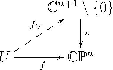
We recall a heuristic idea of this approach known under the name of:

Penrose twistor program. Construct for a given Riemannian manifold M the twistor bundle π : Z → M, where Z is an almost complex manifold and π is a smooth submersion. This bundle should establish a bijective correspondence between:

$$\left\{\begin{array}{l}\text{Riemannian geometry}\\ \text{objects on}M\end{array}\right\}\iff \left\{\begin{array}{l}\text{holomorphic geometry}\\ \text{objects on}Z\end{array}\right\}$$

With the help of this twistor bundle, one can study the real geometry of the Riemannian manifold M via the complex geometry of its twistor space Z.

This formulation of the Penrose twistor program was given in the paper by Atiyah–Hitchin–Singer [12], where a concrete construction of a twistor bundle π : Z → M over an arbitrary even-dimensional Riemannian manifold M was also proposed. To explain this, let us start with a particular, but very important example of the four-dimensional sphere M = S⁴.

3.2. Hopf Bundle

Consider the Hopf bundle over S⁴ of the form:

$$\pi :{\mathbb{P}}^3\stackrel{ℂ{\mathbb{P}}^1}{\to }{S}^4$$

where ℙ³ is the three-dimensional complex projective twistor space. This bundle is the complex version of the Hopf bundle $\pi :S^7\stackrel{S^3}{\to }{S}^4$ In order to see that, we pull back the map π to S⁷ ⊂ ℂ⁴, using the bundle ${ℂ}^4\stackrel{{ℂ}^1}{\to }{\mathbb{P}}^3$, associating with a point of the space ℂ⁴ the complex line, passing through this point. The bundle:

$$\pi :S^7\stackrel{S^3}{\to }{S}^4$$

where ℙ³ is the three-dimensional complex projective twistor space. This bundle is the complex version of the Hopf bundle $\pi :S^7\stackrel{S^3}{\to }{S}^4$. In order to see that, we pull back the map π to S⁷ ⊂ ℂ⁴, using the bundle ${ℂ}^4\stackrel{{ℂ}^1}{\to }{\mathbb{P}}^3$, associating with a point of the space ℂ⁴ the complex line, passing through this point. The bundle:

$$\pi :S^7\stackrel{S^3}{\to }{S}^4$$

with fiber S³ is the quaternion analogue of the Hopf bundle $\pi :S^3\stackrel{S^1}{\to }{S}^2$, which can be also constructed from the complex bundle ${ℂ}^2\stackrel{{ℂ}^1}{\to }{\mathbb{P}}^1$.

The restriction of π to the Euclidean four-space ℝ⁴ = S⁴\{∞} coincides with the bundle:

$$\pi :{\mathbb{P}}^3\backslash {\mathbb{P}}_{\infty }^1\to {ℝ}^4$$

where the omitted complex projective line ${\mathbb{P}}_{\infty }^1$ is identified with the fiber π⁻¹(∞) at ∞ ∈ S⁴.

This bundle has the following geometric interpretation due to Atiyah (cf. [13]). Namely, the space ${\mathbb{P}}^3\backslash {\mathbb{P}}_{\infty }^1$ is foliated by parallel projective planes ℙ² intersecting in ℙ³ on the projective line ${\mathbb{P}}_{\infty }^1$. Consider the fiber π⁻¹(p) of our bundle at p ∈ ℝ⁴. With any point z ∈ π⁻¹(p) of this fiber, we can associate a complex structure J_z on the tangent space T_p ℝ⁴ ≅ ℝ⁴ by identifying (with the help of the tangent map π_∗) this space with the complex plane from our family, going through z. In this way, the fiber π⁻¹(p) of the twistor bundle at p is identified with the space of complex structures on the tangent space T_pℝ⁴ compatible with the metric.

3.3. Atiyah–Hitchin–Singer Construction

We extend now this construction to an arbitrary even-dimensional Riemannian manifold M. Consider the bundle $\pi :\mathcal{J}(M)\to M$ of Hermitian structures on M with fiber at p ∈ M given by the space $\mathcal{J}(T_{p}M)\cong \mathcal{J}({ℝ}^{2n})$ of Hermitian structures on the tangent space T_pM.

Note that a Hermitian structure on the even-dimensional Euclidean space ℝ²ⁿ is a complex structure on ℝ²ⁿ, given by a skew-symmetric linear operator J with the square J² = −I. The space of such structures, denoted by $\mathcal{J}({ℝ}^{2n})$, is identified with the homogeneous space:

$$\mathcal{J}({ℝ}^{2n})\cong \mathcal{O}(2n)/U(n)$$

which is the union of two copies of the homogeneous space SO(2n)/U(n).

The bundle $\pi :\mathcal{J}(M)\to M$ may be identified with the bundle

$$\mathcal{J}(M)=\mathcal{O}(M){\times }_{\mathrm{o}(2n)}\mathcal{J}({ℝ}^{2n}).$$

This bundle will play the role of the twistor bundle over M. We show, first of all, that $\mathcal{J}(M)$ has a natural almost complex structure.

The Riemannian connection on M generates a natural connection on the principal O(2n)-bundle $\mathcal{O}(M)\to M$, which determines the vertical-horizontal decomposition of the associated bundle $\mathcal{J}(M)$:

$$T\mathcal{J}(M)=V\oplus H.$$

We introduce an almost complex structure ${\mathcal{J}}^1$ on $\mathcal{J}(M)$ by setting:

$${\mathcal{J}}^1={\mathcal{J}}^v\oplus {\mathcal{J}}^h.$$

The value of the horizontal component ${\mathcal{J}}_z^v\in \mathrm{End}(V_z)$J ^hz at a point $z\in \mathcal{J}(M)$ coincides with the canonical complex structure on the complex homogeneous space V_z ≅ O(2n)/U(n). The value of the horizontal component ${\mathcal{J}}_z^h\in \mathrm{End}(H_z)$ at z coincides with the complex structure J(z) ↔ z on the space H_z, identified with T_π(z)M by the map π_*. Recall that the fiber π⁻¹(p) of the bundle $\mathcal{J}(M)\to M$ at the point p = π(z) ∈ M consists of Hermitian structures on T_pM, and we denote by J(z) the Hermitian structure on T_pM, corresponding to the point z ∈ π⁻¹(p).

The constructed almost complex structure ${\mathcal{J}}^1$ on $\mathcal{J}(M)$ converts the space $\mathcal{J}(M)$ into an almost complex manifold. This structure was proposed by Atiyah–Hitchin–Singer in [12]. We shall demonstrate now how one can use it for the construction of harmonic spheres in Riemannian manifolds.

3.4. Harmonic Spheres in Riemannian Manifolds

We start from some heuristic considerations. Recall that, according to the Penrose twistor program, one can reduce any problem of the Riemannian geometry on a given Riemannian manifold M to some problem of the complex geometry on the twistor space $Z=\mathcal{J}(M)$. If we believe in this Penrose thesis, we may expect that harmonic spheres φ : S → M in M should arise from pseudoholomorphic spheres $\psi :S\to (Z,{\mathcal{J}}^1)$ as projections of these maps to M, i.e., φ = π ○ ψ:

This is almost true. It turns out that projections of pseudoholomorphic spheres ψ : S → Z to M do satisfy differential equations of second order on M; however, these equations are not harmonic, but ultrahyperbolic; in other words, harmonic equations with the “wrong” signature (n, n) instead of the required signature (2n, 0). For this reason, if we want, justifying the Penrose program, to construct harmonic spheres φ : S → M as projections of pseudoholomorphic spheres ψ : S → Z, then we should change the definition of the almost complex structure on the twistor space $Z=\mathcal{J}(M)$. Namely, in terms of the vertical-horizontal decomposition:

$$T\mathcal{J}(M)=V\oplus H$$

the required almost complex structure ${\mathcal{J}}^2$ on $\mathcal{J}(M)$ should be defined as:

$${\mathcal{J}}^2=(-{\mathcal{J}}^v)\oplus {\mathcal{J}}^h.$$

This almost complex structure on $\mathcal{J}(M)$ was introduced by Eells and Salamon (cf. [14]) and is suitable for the twistor construction of harmonic maps.

Concerning the integrability properties of the introduced almost complex structures, we have the following:

Theorem 3 (Rawnsley, cf. [15]). The almost complex structure${\mathcal{J}}^1$ on the bundle$\mathcal{J}(M)$ is integrable ⇔ M is conformally flat, i.e., N is conformally equivalent to a flat space.

The second almost complex structure ${\mathcal{J}}^2$ on $\mathcal{J}(M)$ is never integrable. We can explain this fact in the following way. It is easy to prove, using the definition of the almost complex structure ${\mathcal{J}}^2$, that if it is integrable, then the local ${\mathcal{J}}^2$-holomorphic curves $f:U\subset ℂ\to \mathcal{J}(M)$ may be only horizontal, i.e., their tangent planes should belong to the horizontal distribution H. On the other hand, if $(\mathcal{J}(M),{\mathcal{J}}^2)$ is a complex manifold, then it should be possible to issue a local complex curve on it in any complex tangent direction.

From first glance, these results on the non-integrability of almost complex structures ${\mathcal{J}}^1$ and ${\mathcal{J}}^2$ may look disappointing, since non-integrable almost complex structures may be quite “bizarre”, having no non-constant holomorphic functions, even locally. However, in our problem, we deal not with holomorphic functions on the twistor space $Z=\mathcal{J}(M)$ (i.e., with holomorphic maps f : Z → ℂ), but with the dual object: holomorphic maps ψ : S → Z from the Riemann sphere S to Z. Such a map ψ is holomorphic with respect to the almost complex structure ${\mathcal{J}}^2$ on Z ⇔ it satisfies the Cauchy–Riemann equation ${\overline{\partial }}_J\psi =0$ with respect to the induced almost complex structure $J:={\phi }^{*}({\mathcal{J}}^2)$ on S. However, on the complex plane ℂ, any almost complex structure is integrable; in particular, the corresponding $\overline{\partial }$-equation has many local solutions.

The next theorem explains how the twistor bundle can be used to construct harmonic spheres.

Theorem 4 (Eells–Salamon, cf. [14]). The bundle of Hermitian structures:

$$\pi :(\mathcal{J}(M{),\mathcal{J}}^2)\to M$$

provided with the almost complex structure${\mathcal{J}}^2$ is a twistor bundle in the following sense: projection φ = π ○ ψ of an arbitrary${\mathcal{J}}^2-\text{holomorphic sphere}$$\psi :S\to \mathcal{J}(M)$ is a harmonic sphere in M.

Having this theorem, one can ask whether a converse statement is true. In other words, if any harmonic sphere φ : S → M, is the projection of some ${\mathcal{J}}^2-\text{holomorphic sphere}$ ψ : S → J (M)? It turns out that a map φ : S → M, obtained by the projection of a ${\mathcal{J}}^2-\text{holomorphic sphere}$ in $\mathcal{J}(M)$, is, apart from being harmonic, also conformal. Recall that a map φ : S → M to a Riemannian manifold (M, g) is conformal if $g\left({{\partial }^{\prime }}_{\phi },\overline{{{{\partial }^{\prime }}^{\prime }}_{\phi }}\right)=0$.

Returning to the problem, formulated above, it can be proven (cf. [15]) that any harmonic conformal map φ : S → M to an oriented Riemannian manifold M is locally the projection of some ${\mathcal{J}}^2-\text{holomorphic curve}$$\psi :U\subset ℂ\to \mathcal{J}(M)$.

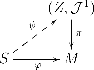
3.5. Twistor Bundles over Riemannian Manifolds

The considered bundle of Hermitian structures $\mathcal{J}(M)\to M$ is not a unique twistor bundle; with the help of which, it is possible to construct harmonic maps. Other twistor bundles are usually obtained from the bundle $\mathcal{J}(M)\to M$ by imposing additional conditions on Hermitian structures in $\mathcal{J}(M)$.

For example, one may consider the Hermitian structures, compatible with orientation, and in this case, we shall obtain the twistor bundle ${\mathcal{J}}^{+}(M)\to M$ with the fiber isomorphic to the homogeneous space SO(2n)/U(n).

Or, for a Kähler manifold M of dimension m, we can consider the complex Grassmann bundle:

$$Z:=G_r(T^{1,0}M)\to M$$

with the fiber at p ∈ M given by the Grassmann manifold $G_r(T_p^{1,0}M)$ of complex subspaces of dimension r in the complex vector space $T_p^{1,0}M$. If we denote by $\mathcal{U}(M)\to M$ the principal U(m)-bundle of unitary frames on M, then:

$$Z=\mathcal{U}(M){\otimes }_{\mathcal{U}(m)}{G}_r({ℂ}^m).$$

A key idea in the construction of different twistor bundles over Riemannian manifolds M is to choose for a class of manifolds M, which we are interested in, an appropriate twistor bundle of complex structures related to the geometry of the manifolds from the considered class. In the next section, we shall introduce twistor bundles over the complex projective and Grassmann manifolds. They may be considered as a particular case of twistor bundles over the homogeneous spaces of the form G/H. Such twistor bundles coincide with the bundles of G-invariant complex structures on G/H.

4. Harmonic Spheres in Projective Spaces

We turn to the description of harmonic spheres φ : S → ℙⁿ in the n-dimensional complex projective space ℙⁿ.

4.1. Explicit Construction of Harmonic Spheres in ℙⁿ

We present first a method of their construction, which formally is not related to the twistor theory (its twistor interpretation will be given later in this section). This method allows one to construct harmonic spheres S → ℙⁿ from the holomorphic spheres in ℙⁿ.

Let f : S → ℙⁿ be a holomorphic sphere in ℙⁿ. The map f is called full if its image is not contained in any proper projective subspace in ℙⁿ. We shall associate with f the spheres f_r : S → G_r+1(ℂⁿ⁺¹) in the Grassmann manifolds G_r+1(ℂⁿ⁺¹) with 0 ≤ r ≤ n.

In the lower hemisphere U = U₀ of S, we consider the local lift f_U of the map f over U. In other words, f_U is the map U → ℂⁿ⁺¹ \ {0}, covering f over U, so that f(z) = π(f_U(z)) for z ∈ U:

Denote ∂^α := ∂^α/∂z^α for α = 1, 2, …, and consider the subspace in ℂⁿ⁺¹ of the form:

$${\theta }_r(p):={\mathrm{span}}_{ℂ}\{{\partial }^{\alpha }{f}_U(z):0\le \alpha \le r\},$$

spanned by the vectors f_U(z), ∂f_U(z), …, ∂^rf_U(z). This subspace does not depend on the choice of the local lift f_U of the curve f and is called the osculating space of f of order r. The same construction applies to the upper hemisphere U_∞ of S.

When the point p ∈ S is changing, the dimension of the osculating space can also change, but for a full sphere, the dimension dim θ_n(p) should be equal to n + 1, at least in one point p ∈ S (hence, in its neighborhood).

Introduce the exceptional set:

$$E=\{p\in S:\dim {\theta }_n(p)<n+1\}$$

and define a holomorphic map f_r : S \ E → G_r+1(ℂⁿ⁺¹) by setting:

$$f_r(p):={\theta }_r(p).$$

The set E for a full holomorphic curve f consists of isolated points; hence, the map f_r may be extended to a holomorphic map:

$$f_r:S\to G_{r+1}({ℂ}^{n+1})$$

which is called the r-th associated curve of the map f. It is evident that f₀ = f, and we set, for convenience, f₋₁ : M → G₀(ℂⁿ⁺¹) equal to zero.

Define for a full holomorphic sphere f : S → ℙⁿ its polar map by setting:

$$g:=f_{n-1}^{\perp }:M\stackrel{f_{n-1}}{\to }{G}_n({ℂ}^{n+1})\stackrel{\perp }{\to }{G}_1({ℂ}^{n+1})={\mathbb{P}}^n$$

where the second map ⊥ associates with a subspace V ∈ G_n(ℂⁿ⁺¹) its orthogonal complement V^⊥. The polar map g : S → ℙⁿ is an anti-holomorphic curve in ℙⁿ, which is connected with f by the orthogonality relations:

$$f_{\alpha }\perp g_{\beta }\text{for}\alpha +\beta \le n-1,$$

or in terms of local lifts:

$$<{\partial }^{\alpha }{f}_U,{\partial }^{\beta }{g}_U>=0\text{for}\alpha +\beta \le n-1.$$

A construction of harmonic spheres in ℙⁿ via holomorphic spheres is given by the following:

Theorem 5 (Eells–Wood, cf. [16]). Let f : S → ℙⁿ be a full holomorphic sphere. For a given r, 0 ≤ r ≤ n, define the map φ : S → ℙⁿ by:

$$\phi (p)=f_{r-1}{(p)}^{\perp }\cap f_r(p),$$

i.e., φ(p) is the orthogonal complement to f_r−1(p) in f_r(p). The equivalent definition:

$$\phi (p)={[f_r{}_{-1}(p)\oplus g_s{}_{-1}(p)]}^{\perp },s:=n-r,$$

where g is the polar map of f. The so-defined map φ : S → ℙⁿ is full and harmonic.

Moreover, the constructed map φ : S → ℙⁿ is complex isotropic. This notion generalizes the notion of conformality. Recall that a map φ : S → M into a Kähler manifold (M, g) is conformal if $g\left({{\partial }^{\prime }}_{\phi },\overline{{{{\partial }^{\prime }}^{\prime }}_{\phi }}\right)=0$. We shall call this map complex isotropic if:

$$g\left({\delta }^{\alpha }{{\partial }^{\prime }}_{\phi },{\delta }^{\beta }\overline{{{{\partial }^{\prime }}^{\prime }}_{\phi }}\right)=0$$

for all α, β with α + β ≥ 1, where δ is the operator, introduced in Section 1. The maps φ : S → ℙⁿ, constructed in the Eells–Wood theorem, are complex isotropic.

The Eells–Wood theorem allows one to construct complex isotropic harmonic spheres φ : S → ℙⁿ from full holomorphic spheres f : S → ℙⁿ. Moreover, the correspondence:

$$\left\{\begin{array}{l}\text{full holomorphic sphere}f:S\to \\ {\mathbb{P}}^n;\text{number}r,0\le r\le n\end{array}\right\}\to \left\{\begin{array}{l}\text{full complex isotropic harmonic}\\ \text{sphere}\phi :S\to {\mathbb{P}}^n\end{array}\right\},$$

constructed in this theorem, is bijective.

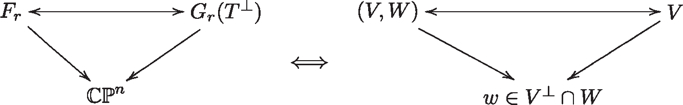
4.2. Interpretation in Terms of Flags

We shall construct explicitly the map, associating with the pair (f, r), where f : S → ℙⁿ is a full holomorphic sphere, the map ψ: S →G_r (T′) where T′ := T^1,0ℙⁿ and G_r := G_r(T^1,0ℙⁿ).

For that, we shall need an interpretation of the bundle G_r(T^1,0ℙⁿ) → ℙⁿ in terms of flag manifolds. Define for 0 ≤ r ≤ n the flag manifold F_r as:

$$F_r:=\{(V;W)\in G_r({ℂ}^{n+1})\times G_{r+1}({ℂ}^{n+1}):V\subset W\}$$

which is a bundle over ℙⁿ of the form:

$$\pi :F_r\to {\mathbb{P}}^n,(V,W)\mapsto V^{\perp }\cap W.$$

This bundle is isomorphic to the Grassmann bundle G_r(T^1,0ℙⁿ) → ℙⁿ. Indeed, the tangent space $T_w^{1,0}({\mathbb{P}}^n)$ at a point w ∈ ℙⁿ is isomorphic to the space of linear maps Hom (w, w^⊥). We associate with an r-dimensional complex subspace H in $T_w^{1,0}({\mathbb{P}}^n)$ the r-dimensional complex subspace in w^⊥, spanned by the images L(w) of linear maps L ∈ H ⊂ Hom(w, w^⊥). In other words, we identify:

$$G_r(T^{1,0}{\mathbb{P}}^n)\leftrightarrow G_r(T^{\perp })$$

where T^⊥ → ℙⁿ is the bundle, obtained from the tautological bundle T → ℙⁿ by taking the fiber-wise orthogonal complement. However, G_r(T^⊥) can be identified with F_r with the help of the correspondence:

In other words, we associate with a pair V ⊂ W from F_r the subspace V ⊂ G_r (ℂⁿ⁺¹) considered as a subspace from [w]^⊥. The subspace W can be reconstructed from V ∈ G_r(T^⊥)_[w] by the formula: W = span{w, V}.

We have shown that the twistor bundle G_r(T^1,0ℙⁿ) → ℙⁿ coincides with the flag bundle F_r → ℙⁿ.

We describe now the map:

$$\left\{\begin{array}{l}(f,r)\text{where}f:S\to {\mathbb{P}}^n\text{is a full}\\ \text{holomorphic sphere}\end{array}\right\}\to \left\{\begin{array}{l}\text{holomorphic sphere}\\ \psi :S\to F_r\end{array}\right\}.$$

Namely, we associate with a full holomorphic sphere f : S → ℙⁿ the map ψ := (f_r−1, f_r) : S → F_r where f_r−1, f_r are the curves, associated with f.

5. Harmonic Spheres in Grassmann Manifolds

We switch now to the twistor description of harmonic spheres in Grassmann manifolds. Here, as in the case of harmonic spheres in ℙⁿ, the role of the twistor spaces will be played by the flag bundles.

5.1. Flag Manifolds

We define first the flag manifolds in ℂⁿ. For that, we fix a decomposition of n into the sum of natural numbers d = r₁ + ⋯ + r_m and denote r := (r₁, …, r_m).

A flag manifold ${ℱ}_{\mathrm{r}}({ℂ}^n)$ of type r in ℂⁿ consists of collections $ℰ=(E_1,\dots ,E_m)$ of mutually orthogonal linear subspaces E_i of dimension r_i in ℂⁿ, such that ℂⁿ = E₁ ⊕ ⋯ ⊕ E_m.

By this definition, a flag is a collection of mutually orthogonal subspaces, rather than a nested sequence of linear subspaces, associated with the standard image of a flag. However, one can easily produce a standard flag (V₁, …, V) in ℂⁿ with V₁ ⊂ ⋯ ⊂ V_m = ℂⁿ from our collection $ℰ=(E_1,\dots ,E_m)$ by setting V_i := E₁ ⊕ ⋯ ⊕ E_i.

In particular, for r = (r, n − r) the flag manifold:

$${ℱ}_{(r,n-r)}({ℂ}^n)=\{ℰ=(E,E^{\perp }):\dim E=r\}=G_r({ℂ}^n)$$

coincides with the Grassmann manifold of r-dimensional subspaces in ℂⁿ.

We have the following homogeneous representation of the flag manifold:

$${ℱ}_{\mathrm{r}}({ℂ}^n)=\mathcal{U}(n)/U(r_1)\times \cdots \times \mathcal{U}(r_n).$$

There is also another, complex homogeneous representation for this manifold:

$${ℱ}_{\mathrm{r}}({ℂ}^n)=\mathrm{GL}(n,ℂ)/{\mathcal{P}}_{\mathrm{r}},$$

where ${\mathcal{P}}_{\mathrm{r}}$ is the parabolic subgroup of blockwise upper-triangular matrices of the form:

$$\left(\begin{array}{lllll}\underset{r_1}{*r_1}\hfill & *\hfill & *\hfill & \cdots \hfill & *\hfill \\ 0\hfill & \underset{r_2}{\begin{array}{||}\hline *\\ \hline\end{array}{r}_2}\hfill & *\hfill & \cdots \hfill & *\hfill \\ ⋮\hfill & \hfill & \ddots \hfill & \hfill & ⋮\hfill \\ 0\hfill & 0\hfill & 0\hfill & \dots \hfill & \stackrel{r_n}{r_n*}\hfill \end{array}\right)$$

with blocks of dimensions r_i × r_i in the boxes.

These representations imply that ${ℱ}_{\mathrm{r}}({ℂ}^n)$ has a natural complex structure, which we denote by ${\mathcal{J}}^1$.

Moreover, ${ℱ}_{\mathrm{r}}({ℂ}^n)$, provided with this complex structure, is a compact Kähler manifold.

In the particular case r = (r, n − r), we obtain the well-known homogeneous representations for the Grassmann manifold:

$$G_r({ℂ}^n)=\mathcal{U}(n)/U(r)\times \mathcal{U}(n-r)=\mathrm{GL}(n,ℂ)/{\mathcal{P}}_{(r,n-r)}.$$

We construct now a series of homogeneous flag bundles over the Grassmann manifold G_r(ℂⁿ). Let $ℱ={ℱ}_{\mathrm{r}}({ℂ}^n)$be the flag manifold of type r = (r₁, …, r_m) in ℂⁿ with the homogeneous representation:

$$ℱ={ℱ}_{\mathrm{r}}({ℂ}^n)=\mathcal{U}(n)/U(r_1)\times \cdots \times \mathcal{U}(r_m).$$

On the Lie algebra level, this representation corresponds to the decomposition of the complexified Lie algebra ${\mathrm{u}}^{ℂ}(n)$ into the direct orthogonal sum:

$$\begin{array}{l}{\mathrm{u}}^{ℂ}(n)\cong \mathrm{gl}(n,ℂ)\cong \overline{{ℂ}^n}\otimes {ℂ}^n\cong ({\overline{E}}_1\oplus \cdots \oplus {\overline{E}}_m)\otimes (E_1\oplus \cdots \oplus E_m)\cong \\ \cong [{\mathrm{u}}^{ℂ}(r_1)\oplus \cdots \oplus {\mathrm{u}}^{ℂ}(r_m)]\oplus \left[\underset{i<j}{\oplus }({\overline{E}}_i{E}_j\oplus {\overline{E}}_j{E}_i)\right].\end{array}$$

(In the latter formula, we have omitted the sign of the tensor product in the expression Ē_iE_j and its conjugate in order to make the formulas more visible. The same rule will be applied in the sequel.)

The above decomposition of the Lie algebra ${\mathrm{u}}^{ℂ}(n)$ implies that the complexified tangent space $T_o^{ℂ}ℱ$ at the origin $o\in ℱ$ coincides with:

$$T_o^{ℂ}ℱ=\underset{i<j}{\oplus }{D}_{ij}^{ℂ}:=\underset{i<j}{\oplus }({\overline{E}}_i{E}_j\oplus {\overline{E}}_j{E}_i).$$

Every component D_ij may be provided with two different complex structures: for one of them, its (1, 0)-subspace coincides with Ē_iE_j; for another, with Ē_jE_i. By the Borel–Hirzebruch theorem [17], any U(n)-invariant almost complex structure J on $ℱ$ is determined by the choice of one of these two complex structures on every D_ij. The almost complex structure ${\mathcal{J}}^1$, for which:

$$T_o^{1,0}ℱ=\underset{i<j}{\oplus }{\overline{E}}_i{E}_j,$$

is called canonical, and it is the only integrable almost complex structure among the introduced ones.

5.2. Flag Bundles

Fix an ordered subset σ ⊂ {1, …, m}. Denote by σ^c the complement of σ in {1, …, m}, and set $r:={\displaystyle {\sum }_{i\in \sigma }{r}_i}$. We can associate with any of such subsets σ a homogeneous bundle:

$${\pi }_{\sigma }:{ℱ}_{\mathrm{r}}({ℂ}^n)=\frac{U(n)}{U(r_1)\times \dots \times U(r_m)}\to \frac{U(n)}{U(r)\times U(n-r)}=G_r({ℂ}^n)$$

by assigning: (E₁, …, E_m) ↦ E = ⊕_i∈σ E_i.

The complexified tangent bundle $T^{ℂ}{ℱ}_{\mathrm{r}}({ℂ}^n)$ is decomposed into the direct sum of vertical and horizontal subbundles. Namely, the vertical subspace at the origin coincides with $\underset{i,j}{\oplus }{D}_{ij}^{ℂ}$, where i < j and either i, j ∈ σ or i, j ∈ σ^c. Respectively, the horizontal subspace at the origin is equal to $\underset{i,j}{\oplus }{D}_{ij}^{ℂ}$, where i < j and either i ∈ σ, j ∈ σ^c or i ∈ σ^c, j ∈ σ.

We introduce by analogy with Eells–Salamon structure from Section 3 an U(n)-invariant almost complex structure ${\mathcal{J}}^2$ on ${ℱ}_{\mathrm{r}}({ℂ}^n)$, setting it equal to ${\mathcal{J}}^1$ on horizontal tangent vectors and $-{\mathcal{J}}^1$ on vertical tangent vectors.

5.3. Twistor Construction of Harmonic Spheres in Grassmannians

Consider the trivial bundle S × ℂⁿ := S × ℂⁿ → S, provided with the standard Hermitian metric on ℂⁿ. Any subbundle E ⊂ S × ℂⁿ of rank r defines a map φ_E : S → G_r(ℂⁿ) by setting: φ_E(p) = the fiber E_p at p ∈ S. Conversely, any map φ : S → G_r(ℂⁿ) defines a subbundle E ⊂ M ×ℂⁿ of rank r.

For a smooth sphere φ : S → G_r(ℂⁿ) in the Grassmannian G_r(ℂⁿ), we denote by π and π^⊥ the orthogonal projections of S × ℂⁿ onto the subbundle E and its orthogonal complement E^⊥. The bundle E is provided with the complex KM-structure, which is determined by the $\overline{\partial }$ -operator:

$${\partial }_E^{"}=\pi \circ \frac{\partial }{\partial }\circ \pi .$$

The inverse image ${\phi }_E^{-1}(T^{ℂ}{G}_r({ℂ}^n))$ of the complexified tangent bundle of the Grassmannian under the map φ_E admits a decomposition:

$${\phi }_E^{-1}(T^{ℂ}{G}_r({ℂ}^n))\cong \overline{E}{E}^{\perp }\oplus \overline{E^{\perp }}E.$$

In terms of this decomposition, the differential of φ_E has local components:

$${A^{\prime }}_E:={\pi }^{\perp }\circ \frac{\partial }{\partial z}\circ \pi ,{A^{″}}_E:={\pi }^{\perp }\circ \frac{\partial }{\partial z}\circ \pi .$$

(In the sequel, we sometimes omit the sign ◦ to simplify the formulas.) In particular, a bundle E ⊂ S×ℂⁿ is holomorphic $\iff {A^{″}}_E=0$, and in this case, the complex KM-structure on E coincides with the complex structure, induced from S × ℂⁿ. The bundle ${A^{\prime }}_E\in \mathrm{Hom}(E,E^{\perp })$ is holomorphic with respect to KM-structures on E and E^⊥.

In general, we call a bundle E ⊂ S × ℂⁿ harmonic if:

$${A^{\prime }}_E\circ {{\partial }^{″}}_E={{\partial }^{″}}_{E^{\perp }}\circ {A^{\prime }}_E.$$

The harmonicity of E is equivalent to the harmonicity of the map φ_E : S → G_r(ℂⁿ). Note also that E is harmonic iff its orthogonal complement E^⊥ is harmonic.

In a more general way, consider an arbitrary collection $ℰ=(E_1,\dots ,E_m)$ of mutually orthogonal subbundles E_i in S × ℂⁿ of rank r_i with r₁ + … + r_m = n, which generates a decomposition of S × ℂⁿ into the direct orthogonal sum:

$$S\times {ℂ}^n=\underset{i=1}{\overset{n}{\oplus }}{E}_i.$$

We call such a collection of subbundles $ℰ=(E_1,\dots ,E_m)$ the moving flag on S. It determines, in the same way as before, a map ${\psi }_{\epsilon }:S\to {ℱ}_{r_1\dots r_m}=ℱ$ by assigning to a point p ∈ S the flag, defined by the subspaces (E_1,p,…, E_m,p). Conversely, any smooth map $\psi :S\to ℱ$ determines a moving flag $ℰ=(E_1,\dots ,E_m)$, where E_i = ψ⁻¹T_i is the pull-back of a natural tautological bundle $T_i\to {ℱ}_{\mathrm{r}}$ : the fiber of T_i at $ℰ\in ℱ$ coincides, by definition, with the subspace E_i for 1 ≤ i ≤ m.

As in the Grassmann case, the differential ψ_ℇ is determined locally by the components:

$${A^{\prime }}_{ij}:={\pi }_i\circ \frac{\partial }{\partial z}\circ {\pi }_j,{A^{″}}_{ij}:={\pi }_i\circ \frac{\partial }{\partial z}\circ {\pi }_j,$$

where π_i : S × ℂⁿ → E_i is the orthogonal projection.

Theorem 6 (Burstall–Salamon, cf. [18]). The homogeneous flag bundle:

$${\pi }_{\sigma }:({ℱ}_{\mathrm{r}}({ℂ}^n),{\mathcal{J}}^2)\to G_r({ℂ}^n)$$

is a twistor bundle, i.e., for any${\mathcal{J}}^2$- holomorphic map$\psi :S\to {ℱ}_{\mathrm{r}}({ℂ}^n)$, its projection φ = π_σ ○ ψ:S → G_r(ℂⁿ) is harmonic.

The converse of the Theorem 6 is also true.

Theorem 7 (Burstall, cf. [19]). Any harmonic map$\phi :S\to G_r({ℂ}^n)$ can be obtained as the projection of a $ℐ$²-holomorphic map$\psi :S\to {ℱ}_{\mathrm{r}}({ℂ}^n)$ with respect to some twistor bundle${\pi }_{\sigma }:{ℱ}_{\mathrm{r}}({ℂ}^n)\to G_r({ℂ}^n)$.

6. Harmonic Spheres in the Hilbert–Schmidt Grassmannian

We switch now to the case of infinite-dimensional Grassmann manifolds and try to extend to this case the methods developed for finite-dimensional Grassmannians in the previous Section.

6.1. Hilbert–Schmidt Grassmannian

We start from the definition of the Hilbert–Schmidt Grassmannian Gr_HS(H) of a complex (separable) Hilbert space H. We take for a model of this Hilbert space the space $L_0^2(S^1,ℂ)$ of square integrable complex-valued functions on the circle S¹ with zero average over S¹.

Suppose that H has a polarization, i.e., a decomposition:

$$H=H_{+}\oplus H_{-}$$

into the direct orthogonal sum of infinite-dimensional closed subspaces. In the case of $H=L_0^2(S^1,ℂ)$, one can take for such subspaces:

$$H_{\pm }=\left\{\gamma \in H:\gamma (z)={\displaystyle \sum _{\pm k>0}{\gamma }_k{z}^k}\right\}.$$

Any bounded linear operator A ∈ L(H) with respect to the given polarization can be written in the block form:

$$A=\left(\begin{array}{cc}a& b\\ c& d\end{array}\right)=\left(\begin{array}{cc}a:H_{+}\to H_{+},& b:H_{-}\to H_{+}\\ c:H_{+}\to H_{-}& d:H_{-}\to H_{-}\end{array}\right).$$

Denote by GL(H) the group of linear bounded operators on H, having a bounded inverse, and introduce the Hilbert–Schmidt group GL_HS(H), consisting of operators A ∈ GL(H), for which the “off-diagonal” terms b and c are Hilbert–Schmidt operators. In other words, the group GL_HS(H) consists of operators A ∈ GL(H), for which the “off-diagonal” terms b and c are “small” with respect to the “diagonal” terms a and d. We denote by U_HS(H) the intersection of GL_HS(H) with the group U(H) of unitary operators in H.

As in the finite-dimensional situation, there is a Grassmann manifold Gr_HS(H), called the Hilbert–Schmidt Grassmannian, associated with the group GL_HS(H).

The Hilbert–Schmidt Grassmannian Gr_HS(H) is the set of all closed subspaces W ⊂ H, such that the orthogonal projection pr₊ : W → H₊ is a Fredholm operator, and the orthogonal projection pr₋ : W → H₋ is a Hilbert–Schmidt operator. Equivalently: a subspace W ∈ Gr_HS(H) iff it coincides with the image of a linear operator w : H₊ → H, such that w₊ := pr₊ ○ w is a Fredholm operator and w₋ := pr₋ ○ w is a Hilbert–Schmidt operator.

In other words, the Hilbert–Schmidt Grassmannian Gr_HS(H) consists of the subspaces W ⊂ H, which differ “little” from the subspace H₊ in the sense that the projection pr₊ : W → H₊ is “close” to an isomorphism and the projection pr₋ : W → H₋ is “small”.

We have the following homogeneous space representation of: Gr_HS(H):

$${\mathrm{Gr}}_{\mathrm{HS}}(H)={\mathcal{U}}_{\mathrm{HS}}(H)/\mathcal{U}(H_{+})\times \mathcal{U}(H_{-}).$$

Since U_HS(H) acts transitively on the Grassmannian Gr_HS(H), we can construct an U_HS(H)-invariant Kähler metric on Gr_HS(H) from an inner product on the tangent space $T_H{}_{{}_{+}}{\mathrm{Gr}}_{\mathrm{HS}}(H)$ at the origin H₊ ∈ Gr_HS(H), invariant under the action of the isotropy subgroup U(H₊)×U(H₋). The tangent space $T_H{}_{{}_{+}}{\mathrm{Gr}}_{\mathrm{HS}}(H)$ coincides with the space of Hilbert–Schmidt operators HS(H₊, H₋), and the invariant inner product on it is given by the formula:

$$(A,B)\mapsto \mathrm{Re}\left\{\mathrm{tr}(A{B}^{†})\right\},A,B\in \mathrm{HS}(H_{+},H_{-}).$$

Note that the imaginary part of the complex inner product tr(AB^†) determines a non-degenerate invariant 2-form on $T_H{}_{{}_{+}}{\mathrm{Gr}}_{\mathrm{HS}}(H)$, which extends to an U_HS(H)-invariant symplectic structure on Gr_HS(H). Hence, we have a Kähler structure on Gr_HS(H), which makes it a Kähler Hilbert manifold.

The evident difficulty, related to the extension of the techniques, developed for finite-dimensional Grassmannians, to the case of Gr_HS(H), is that the subspaces W ∈ Gr_HS(H) are infinite-dimensional. In this sense, they all have the same infinite “dimension”, which does not allow one to compare them. However, there is a replacement of the notion of dimension, which is more helpful for the study of such subspaces. Namely, one can compare them by their “relative dimension”, called also the “virtual dimension”.

In more detail, the manifold Gr_HS(H) has a countable number of connected components, numerated by the index of the Fredholm operator w₊ for a subspace W ∈ Gr_HS(H), coinciding with the image of a linear operator w : H₊ → H. We say that a subspace W has the virtual dimension d, if the index of w₊ is equal to d. Denote by G_r(H) the component of Gr_HS(H), consisting of subspaces W of virtual dimension r. Then, we have the following decomposition of Gr_HS(H) into the disjoint union of its connected components G_r(H):

$${\mathrm{Gr}}_{\mathrm{HS}}(H)={\displaystyle \underset{r}{\cup }{\mathrm{G}}_r(H)}.$$

Due to this decomposition, the study of harmonic maps of Riemann surfaces into Gr_HS(H) is reduced to the study of harmonic maps into Grassmannians G_r(H) of virtual dimension r, which may be carried on along the same lines, as in the case of the Grassmann manifold $G_r({ℂ}^n)$.

6.2. Harmonic Spheres in Hilbert–Schmidt Grassmannian

Denote by S × H := S × H → S the trivial bundle where H is a complex Hilbert space provided with polarization. We consider the subbundles E ⊂ S × H with fibers E_p ∈ Gr_HS(H) for p ∈ S. As for finite-dimensional Grassmannians, any bundle E of this type defines a map φ_E : S → Gr_HS(H), and conversely, any map φ : S → Gr_HS(H) defines a subbundle E ⊂ S × Gr_HS(H).

Consider a smooth sphere in the Grassmannian Gr_HS(H). Denote by π and π^⊥ the orthogonal projections of S × H onto the subbundle E and its orthogonal complement E^⊥, respectively. The bundle E is provided with the complex KM-structure, which is determined by the $\overline{\partial }$-operator:

$${{\partial }^{″}}_E=\pi \circ \frac{\partial }{{\partial }_{\overline{z}}}\circ \pi .$$

The inverse image ${\phi }_E^{-1}(T^{ℂ}{\mathrm{Gr}}_{\mathrm{HS}}(H))$ of the complexified tangent bundle of Gr_HS(H) under the map φ_E admits the decomposition:

$${\phi }_E^{-1}(T^{ℂ}{\mathrm{Gr}}_{\mathrm{HS}}(H))\cong \overline{E}{E}^{\perp }\oplus \overline{E^{\perp }}E.$$

In terms of this decomposition, the differential of φ_E has local components:

$${A^{\prime }}_E:={\pi }^{\perp }\circ \frac{\partial }{\partial z}\circ \pi ,{A^{″}}_E:={\pi }^{\perp }\circ \frac{\partial }{\partial z}\circ \pi .$$

In particular, a bundle E ⊂ M × H is holomorphic iff ${A^{″}}_E=0$, and in this case, the KM-structure on E coincides with the complex structure, induced from M × H. Then:

$$\begin{array}{l}0={\pi }^{\perp }\left[\frac{\partial }{\partial z}\left(\pi +{\pi }^{\perp }\right)\frac{\partial }{\partial z}-\frac{\partial }{\partial z}\left(\pi +{\pi }^{\perp }\right)\frac{\partial }{\partial z}\right]\pi =\\ ={A^{\prime }}_E{{\partial }^{″}}_E+{{\partial }^{\prime }}_{E^{\perp }}{A^{″}}_E-{A^{″}}_E{{\partial }^{\prime }}_E-{{\partial }^{″}}_{E^{\perp }}{A^{\prime }}_E={A^{\prime }}_E{{\partial }^{″}}_E-{{\partial }^{″}}_{E^{\perp }}{A^{\prime }}_E.\end{array}$$

In other words, ${A^{\prime }}_E\in$ Hom(E, E^⊥) is holomorphic with respect to the KM-structures on E and E^⊥.

As in the finite-dimensional situation, we call a bundle E ⊂ M × H harmonic if:

$${A^{\prime }}_E\circ {{\partial }^{″}}_E={{\partial }^{″}}_{E^{\perp }}\circ {A^{\prime }}_E$$

and the harmonicity of E is equivalent to the harmonicity of the map φ_E : S → G_r(H).

Now, we generalize this situation to the maps into infinite-dimensional flag manifolds.

Introduce first the Hilbert–Schmidt flag manifolds. For that, fix an n-tuple r = (r₁, …, r_n) of integers. The Hilbert–Schmidt flag manifold F_r(H) consists of the flags of the form:

$$\epsilon \equiv (E_1,\dots E_m)$$

where E_k ≡ W_in, E_l ≡ W_out are closed infinite-dimensional subspaces in H and:

$$E_1,\dots ,E_{k-1},E_{k+1},\dots ,E_{l-1},E_{l+1},\dots ,E_m$$

are finite-dimensional subspaces having the following properties:

• the projection pr₊ : W_in → H₊ is a Fredholm operator of index r_k, while the projection pr₋ : W_in → H₋ is a Hilbert–Schmidt operator;
• the projection pr₋ : W_out → H₋ is a Fredholm operator of index r_l, while the projection pr₊ : W_out → H₊ is a Hilbert–Schmidt operator;
• E_i with i = 1, …, k − 1, k + 1, …, l − 1, l + 1, …, m are r_i-dimensional vector subspaces in H;
• all subspaces E_i with i = 1, …, m are pairwise orthogonal, and their direct sum is equal to H: E₁ ⊕…⊕ E_m = H.

To simplify the notation, we say that ε = (E₁,…E_m) is a virtual flag of virtual dimension r = (r₁, …, r_m) having in mind that r_k (resp. r_l) are integers, equal to the virtual dimension of E_k = W_in (resp. E_l = W_out), while other r_i’s are positive integers, equal to the dimensions of E_i’s for i ≠ k, l.

The tangent space to F_r(H) at the origin, as in the finite-dimensional case, is the direct sum of four different terms:

$$\begin{array}{l}{T}^{ℂ}(F_{\mathrm{r}}(H))\cong \underset{1\le i,j\ne k,l,i<j\le m}{\oplus }\left[{\overline{E}}_i{E}_j\oplus {\overline{E}}_j{E}_i\right]\oplus \underset{1\le i\le m,i\ne k}{\oplus }\left[{\overline{W}}_{\mathrm{in}}{E}_i\oplus {\overline{E}}_i{W}_{\mathrm{in}}\right]\\ \oplus \underset{1\le i\le m,i\ne l}{\oplus }\left[{\overline{W}}_{\mathrm{out}}{E}_i\oplus {\overline{E}}_i{W}_{\mathrm{out}}\right]\oplus \left[{\overline{W}}_{\mathrm{in}}{W}_{\mathrm{out}}\oplus {\overline{W}}_{\mathrm{out}}{W}_{\mathrm{in}}\right].\end{array}$$

The tangent space to Gr_HS(H) looks the same if we set E_i = 0 for all E_i’s, except for i = k, l.

Generalizing the finite-dimensional situation, we consider an arbitrary collection ε = (E₁, …, E_m) of mutually orthogonal subbundles E_i in M × H of virtual dimension r = (r₁, …, r_m), generating the decomposition of S × H into the direct orthogonal sum:

$$S\times H=\underset{i=1}{\overset{n}{\oplus }}{E}_i.$$

We call such a collection of subbundles ε = (E₁, …, E_m) the moving flag on S. It determines, in the same way as before, a map ψ_ε : S → F_r(H) ≡ $ℱ$ by assigning to a point p ∈ S the flag defined by the subspaces (E_1,p, …, E_m,p). Conversely, any smooth map ψ : S → $ℱ$ determines a moving flag ε = (E₁, …, E_m), where E_i = ψ⁻¹T_i is the pull-back of a natural tautological bundle T_i → F_r(H): the fiber of T_i at ε ∈ $ℱ$ coincides, by definition, with the subspace E_i for 1 ≤ i ≤ m.

As for finite-dimensional Grassmannians, the differential ψ_ε is determined locally by the components:

$${A^{\prime }}_{ij}={\pi }_i\circ \frac{\partial }{\partial z}\circ {\pi }_j,{A^{″}}_{ij}={\pi }_i\circ \frac{\partial }{\partial z}\circ {\pi }_j,$$

where π_i : S × H → E_i is the orthogonal projection. Note that, by construction, ${A^{″}}_{ij}=-{\left({A^{\prime }}_{ji}\right)}^{*}$.

Each of the subbundles E_i of the trivial bundle S × H is provided with the KM-structure, which coincides with the complex structure, induced from S × H. Furthermore, the components ${A^{\prime }}_{ij}$, ${A^{″}}_{ij}$ satisfy the same harmonicity and holomorphicity conditions as in the finite-dimensional case.

We introduce now an almost complex structure on the Hilbert–Schmidt flag bundle F_r(H), analogous to the almost complex structure ${\mathcal{J}}_{\sigma }^2$. As in the finite-dimensional situation, an almost complex structure on F_r(H) is fixed by choosing the (1, 0)-component in each of the summands of:

$$T^{ℂ}(F_{\mathrm{r}}(H))\cong \underset{1\le i<j\le m}{\oplus }\left[{\overline{E}}_i{E}_j\oplus {\overline{E}}_j{E}_i\right].$$

(3)

To define an almost complex structure ${\mathcal{J}}_{\sigma }^2$, we fix an ordered subset σ ⊂ {1, …, m}. Then, for the associated almost complex structure ${\mathcal{J}}_{\sigma }^2$, we choose for i, j ∈ {1, …, m}, i < j, the (1, 0)-component in the (i, j)-summand in (3), equal to Ē_jE_i if i, j ∈ σ or i, j ∉ σ and to Ē_iE_j if i ∈ σ, j ∉ σ or i ∉ σ, j ∈ σ.

We construct now the Hilbert–Schmidt flag bundle over the Hilbert–Schmidt Grassmannian. Suppose That σ is a fixed ordered subset in {1, …, m}, and set $r={\displaystyle {\sum }_{i\in \sigma }{r}_i}$ Then, we define the Hilbert–Schmidt flag bundle:

$${\pi }_{\sigma }:F_{\mathrm{r}}(H)\to G_r(H)$$

by mapping:

$$ℰ=(E_1,\dots ,E_m)\mapsto E:=\underset{i\in \sigma }{\oplus }{E}_i.$$

With this definition, we have the following:

Theorem 8 (Beloshapka–Sergeev, cf. [2]). Let σ be an ordered subset in {1, …, m}, such that k ∈ σ, l ∉ σ. Then, the map π_σ of the Hilbert–Schmidt flag manifold F_r(H), provided with the almost complex structure${\mathcal{J}}_{\sigma }^2$ to G_r(H):

$${\pi }_{\sigma }:F_{\mathrm{r}}(H)\to G_r(H)$$

is a twistor bundle, i.e., for any${\mathcal{J}}_{\sigma }^2$-holomorphic map ψ : S → F_r(H), its projection φ = π_σ ○ ψ : S → G_r(H) is harmonic.

The converse of this theorem is also true.

Theorem 9 (Beloshapka–Sergeev, cf. [2]). Let φ : S → G_r(H) be a harmonic sphere. Then, there exist a Hilbert–Schmidt flag bundle:

$${\pi }_{\sigma }:F_{\mathrm{r}}(H)\to G_r(H)$$

and a${\mathcal{J}}_{\sigma }^2$-holomorphic map ψ : S → F_r(H), such that φ coincides with the projection π_σ ○ ψ of the map ψ.

7. Harmonic Maps into Loop Spaces

We can apply the above results to the study of harmonic maps into the loop spaces ΩG of compact Lie groups G by embedding these loop spaces into the Hilbert–Schmidt Grassmannian. At the end of this section, we explain, why this case is particularly interesting for us.

7.1. Loop Spaces

Denote by LG = C^∞(S¹, G) the loop group of G, i.e., the space of C^∞-smooth maps S¹ → G, where S¹ is identified with the unit circle in ℂ. It is a Lie–Frechet group with respect to the pointwise multiplication, modeled on the loop algebra $L\mathfrak{g}=C^{\infty }(S^1,\mathfrak{g})$, where $\mathfrak{g}$ is the Lie algebra of the group G. The loop space ΩG of the group G (or the based loop space) is the homogeneous space of the group LG of the form:

$$\mathrm{\Omega }G=LG/G$$

where the group G in the denominator is identified with the subgroup of constant maps S¹ → g₀ ∈ G. Note that the loop space ΩG may be identified with the space of based maps in LG, sending 1 ∈ S¹ to the unit e of the group G and, so, inheriting a Frechet manifold structure from the loop group LG.

The loop group LG acts on ΩG by left translations. Denote by o the origin in ΩG, represented by the class of constant maps: o = [G]. The tangent space of ΩG at the origin o is identified with the space $\Omega \mathfrak{g}=L\mathfrak{g}/\mathfrak{g}$. We represent vectors of the tangent space T_o(ΩG) by their Fourier series: an arbitrary vector ξ of the complexified tangent space $T_o^{ℂ}(\Omega G)=T_o(\Omega G)\otimes ℂ$, having a Fourier decomposition of the form:

$$\xi ={\displaystyle \sum _{k\ne 0}{\xi }_k{e}^{ik\theta }}$$

where the coefficients ξ_k belong to the complexified Lie algebra ${\mathfrak{g}}^{ℂ}$. A vector ξ ∈ T_o(ΩG) iff ${\xi }_{-k}={\overline{\xi }}_k$.

The loop space ΩG has a natural symplectic structure, invariant under the action of the loop group LG on ΩG. Due to the invariance, it is sufficient to define its restriction to $T_o(\Omega G)=\Omega \mathfrak{g}$. For that, we fix an invariant inner product < ·, · > on the Lie algebra $\mathfrak{g}$ and consider a two-form ω on $L\mathfrak{g}$ of the form:

$$\omega (\xi ,\eta )=\frac{1}{2\pi }{\displaystyle {\int }_0^{2\pi }<\xi (\theta ),{\eta }^{\prime }(\theta )>d\theta ,\xi ,\eta \in L\mathfrak{g}.}$$

This formula defines a left-invariant closed two-form on LG, subject to the condition: ω(ξ, η) = 0 iff at least one of the maps ξ, η is constant. Hence, it can be pushed down to a left-invariant two-form on $\Omega \mathfrak{g}$, which is non-degenerate and closed and, so, generates a symplectic structure on ΩG (cf. [20,21]).

An invariant complex structure on ΩG is provided by the “complex” representation of ΩG = LG/G as a homogeneous space of the complex Lie–Frechet group $L{G}^{ℂ}=C^{\infty }(S^1,G^{ℂ})$, where $G^{ℂ}$ is the complexification of the Lie group G. This representation has the form:

$$\mathrm{\Omega }G=L{G}^{ℂ}/L^{+}{G}^{ℂ}$$

(4)

where $L^{+}{G}^{ℂ}=\mathrm{Hol}(\mathrm{\Delta }\mathrm{a},G^{ℂ})$ is a subgroup of $L{G}^{ℂ}$, consisting of the maps $S^1\to G^{ℂ}$, which can be extended smoothly to holomorphic maps of the disc $\mathrm{\Delta }\mathrm{a}:=\left\{\right|z|<1\}\to G^{ℂ}$.

The invariant complex structure J¹ on ΩG, induced by the complex representation (4), has a simple meaning in terms of Fourier series. Namely, the restriction of J¹ to the complexified tangent space $T_o^{ℂ}(\Omega G)=\Omega {\mathfrak{g}}^{ℂ}$ at the origin is given by the following formula:

$$\xi ={\displaystyle \sum _{k\ne 0}{\xi }_k{e}^{ik\theta }}\mapsto J^1\xi =-i{\displaystyle \sum _{k>0}{\xi }_k{e}^{ik\theta }}+i{\displaystyle \sum _{k<0}{\xi }_k{e}^{ik\theta }}.$$

The introduced symplectic and complex structures on ΩG are compatible in the sense that ω(J¹ξ, J¹η) = ω(ξ, η) for all ξ, η ∈ T_o(ΩG), and the symmetric form:

$$g^1(\xi ,\eta ):=\omega (\xi ,J^1\eta )\mathrm{on}{T}_o(\mathrm{\Omega }G)\times T_o(\mathrm{\Omega }G)$$

is positive definite. Therefore, this form extends to an invariant Riemannian metric g¹ on ΩG (due to the invariance of ω and J¹). In other words, the loop space ΩG is a Kähler Frechet manifold, provided with the Kähler metric g¹.

7.2. Harmonic Spheres in Loop Spaces

We shall study harmonic spheres in the loop spaces ΩG by embedding isometrically ΩG into the Hilbert–Schmidt Grassmannian Gr_HS(H).

Assume that G is a subgroup of U(n) for some n. Then, we have an isometric embedding:

$$LG\to {\mathcal{U}}_{\mathrm{HS}}(H),$$

given by the map:

$$\gamma \in LG=C^{\infty }(S^1,G)\to M_{\gamma }\in {\mathcal{U}}_{\mathrm{HS}}(H),$$

where the multiplication operator M_γ is defined by:

$$f\in H=L_0^2(S^1,{ℂ}^n)\mapsto (M_{\gamma }f)(z):=\gamma (z)f(z)\text{for}z\in S^1.$$

It is easy to check that M_γ ∈ U_HS(H) if γ is smooth.

The constructed embedding of the loop group LG into U_HS(H) induces an isometric embedding:

$$\mathrm{\Omega }G\to {\mathrm{Gr}}_{\mathrm{HS}}(H).$$

Therefore, we can consider harmonic spheres S → ΩG as taking values in Gr_HS(H), thus reducing their study to the study of harmonic spheres S → Gr_HS(H), considered above.

8. Yang–Mills Fields and Instantons

8.1. Yang–Mills Equations

Let G be a compact Lie group (gauge group). A gauge potential on ℝ⁴ is a connection A in a principal G-bundle over ℝ⁴ identified with a one-form on ℝ⁴ with values in the Lie algebra $\mathfrak{g}$ of G. In the case when G coincides with the group U(n) of unitary (n × n)-matrices, this form can be written as:

$$A={\displaystyle \sum _{\mu =1}^4{A}_{\mu }(x)d{x}_{\mu }}$$

where x = (x₁, x₂, x₃, x₄) are coordinates on ℝ⁴ and coefficients A_µ(x) are smooth functions on ℝ⁴ with values in the algebra of skew-Hermitian (n × n)-matrices.

A gauge G-field F is the curvature of the connection A given by the two-form on ℝ⁴ with values in the Lie algebra $\mathfrak{g}$:

$$F=DA=dA+\frac{1}{2}[A,A]$$

where $D:{\Omega }^1({ℝ}^4,\mathfrak{g})\to {\Omega }^2({ℝ}^4,\mathfrak{g})$ is the exterior covariant derivative generated by the connection A. In the case G = U(n), this form is written as:

$$F={\displaystyle \sum _{\mu ,\nu =1}^4{F}_{\mu \nu }(x)d{x}_{\mu }\wedge d{x}_{\nu }}$$

where:

$$F_{\mu \nu }={\partial }_{\mu }{A}_{\nu }-{\partial }_{\nu }{A}_{\mu }+[A_{\mu },A_{\nu }]$$

with ∂_µ := ∂/∂x_µ, µ = 1, 2, 3, 4.

Introduce the Yang–Mills action functional given by the formula:

$$S(A)=\frac{1}{2}{\displaystyle {\int }_{{ℝ}^4}{\Vert F\Vert }^2{d}^{4}x}$$

where the norm ║F║ is computed with the help of a given fixed invariant inner product on the Lie algebra g. In the case G = U(n), one can take for such a product 〈X, Y〉 := −tr(XY). In this case, the formula for the action S(A) will be rewritten in the form:

$$S(A)=\frac{1}{2}{\displaystyle {\int }_{{ℝ}^4}tr({}_{*}F\wedge F)}$$

where _* is the Hodge star-operator on ℝ⁴.

The functional S(A) is invariant under gauge transformations given by the smooth mappings g : ℝ⁴ → G, tending to the unit e ∈ G at infinity. Under the action of these transformations, gauge potentials and fields transform according to the following formulas:

$$A\mapsto A_g:=g^{-1}dg+g^{-1}Ag,g:F\mapsto F_g:=g^{-1}Fg$$

where the group G acts on its Lie algebra $\mathfrak{g}$ by the adjoint representation. In the case G = U(1), a gauge transform is given by the multiplication by the gauge factor g(x) = e^iθ(x), so that the corresponding gauge potential transformation coincides with the gradient transform A ⟼ A − idθ, while the gauge field F does not change.

A gauge field F is called the Yang–Mills field if it is extremal for the action functional S(A) and has finite Yang–Mills action S(A) < ∞. The corresponding gauge potential A is called the Yang–Mills connection.

The Euler–Lagrange equation for the functional S(A) have the form:

$$D*F=0$$

where $D*:{\Omega }^2({ℝ}^4,\mathfrak{g})\to {\Omega }^1({ℝ}^4,\mathfrak{g})$ is the operator formally adjoint to D. In the case ℝ⁴, it coincides with D* = − _* D_*, where _* is the Hodge operator, so that the Euler–Lagrange equations for S(A) are rewritten in the form:

$$D*F=0.$$

The obtained equation is called the Yang–Mills equation and is often supplemented with the Bianchi identity:

$$DF=0$$

which is satisfied automatically for gauge fields F.

A gauge field F is called self-dual (resp. anti-self-dual) if:

$${}_{*}F=F(\mathrm{resp}{.}_{*}F=-F).$$

The Bianchi identity implies immediately that solutions of the duality equations:

$${}_{*}F=\pm F$$

satisfy automatically the Yang–Mills equation.

If we write down the form F as the sum:

$$F=F_{+}+F_{-},$$

where $F_{\pm }=\frac{1}{2}({}_{*}F\pm F)$, then the formula for the Yang–Mills action will rewrite as:

$$S(A)=\frac{1}{2}{\displaystyle {\int }_{{ℝ}^4}\left({\Vert F_{+}\Vert }^2+{\Vert F_{-}\Vert }^2\right)d^{4}x.}$$

For the gauge fields F with finite Yang–Mills action, the quantity:

$$k(A)=\frac{1}{8{\pi }^2}{\displaystyle {\int }_{{ℝ}^4}\left(-{\Vert F_{+}\Vert }^2+{\Vert F_{-}\Vert }^2\right)d^{4}x}$$

turns out to be an integer-valued topological invariant called the topological charge of the field F. If we extend, using the Uhlenbeck compactness theorem, a connection A with finite Yang–Mills action to a connection in some associated vector bundle E over the compactification S⁴ of ℝ⁴, then this invariant will be expressed in terms of Chern classes of this bundle. For example, in the case of G = SU(2), it coincides with the second Chern class.

Comparing the above formulas for the action S(A) and topological charge k(A), we arrive at the estimate:

$$S(A)\ge 4{\pi }^2\left|k(A)\right|.$$

From the same formulas, we see that the minimum of the action S(A) on the topological class of gauge fields with finite Yang–Mills action and fixed topological charge k(A) = k is equal to 4π²|k| and is attained for k > 0 on anti-selfdual fields, while for k < 0, it is attained on self-dual fields.

An anti-self-dual field with finite Yang–Mills action is called the instanton and a self-dual field with finite Yang–Mills action is called the anti-instanton.

Instantons and anti-instantons realize the local minima of the action S(A); however, this functional has also non-minimal critical points (cf. [22–25]).

8.2. Yang–Mills Moduli Spaces

One of the main goals of Yang–Mills theory is the investigation of the structure of the moduli space $ℳ$_k of Yang–Mills fields with fixed topological charge k given by the quotient:

$${ℳ}_k=\frac{\left\{\mathrm{Yang}–\text{Mills fields with fixed topological charge}k\right\}}{\left\{\text{gauge transforms}\right\}}$$

We are still far from the complete understanding of the structure of this space; however, an analogous problem for the instantons, i.e., the description of the moduli space of instantons on ℝ⁴, was solved by Atiyah, Drinfeld, Hitchin and Manin (cf. below) with the help of the twistor approach presented in the next section.

The moduli space ${\mathcal{N}}_k$ of instantons with the fixed topological charge k, which is defined as:

$${\mathcal{N}}_k=\frac{\left\{\text{G-instantons on}{ℝ}^4\text{with topological charge}k\right\}}{\left\{\text{gauge transforms}\right\}},$$

admits the following interpretation in terms of the Hopf bundle ${\mathbb{P}}^3\backslash {\mathbb{P}}_{\infty }^1\to {ℝ}^4$. According to the theorem of Atiyah–Ward [3], there exists a bijective correspondence between:

$$\left\{\begin{array}{c}\text{moduli space of}\\ G\text{-instantons on}{ℝ}^4\end{array}\right\}\leftrightarrow \left\{\begin{array}{c}\text{equivalence classes of based holomorphic}\\ G^{ℂ}\text{-bundles over}ℂ{\mathbb{P}}^3,\text{trivial on}\pi \text{-fibers}\end{array}\right\}.$$

Here, G^ℂ -bundle over ℂℙ ³ is called based if it is provided with a fixed trivialization on ${\mathbb{P}}_{\infty }^1={\pi }^{-1}(\infty )$.

Using this twistor interpretation of instantons, Atiyah, Drinfeld, Hitchin and Manin gave a full description of the moduli space of instantons known under the name of ADHM-construction (cf. [4]).

8.3. Twistor Description of Yang–Mills Fields

In order to extend these results to arbitrary Yang–Mills fields, we would like to have the twistor interpretation of these fields. Such an interpretation was proposed in the papers by Manin [5], Witten [6] and Isenberg-Green-Yasskin [7]. To present their construction, denote by (ℙ³)* the dual projective space identified with the space of complex projective planes ℙ² in ℙ³. Consider the space F of flags in ℙ³ × (ℙ³)^* consisting of pairs: (point; plane, containing this point). In homogeneous coordinates ([z];[ξ]) on ℙ³ × (ℙ³)^*, this space is identified with the subspace:

$$Q=\left\{([z];[\xi ]):(z,\xi )=0\right\}$$

where (·, ·) denotes the natural pairing between ℙ³ and (ℙ³)^*. The twistor construction, mentioned above, gives a description of holomorphic Yang–Mills fields on the complexified space ℂS⁴ identified with the Grassmann manifold G₁(ℙ³) ≡ G₂(ℂ⁴). Namely, such fields correspond to the equivalence classes of holomorphic G^ℂ -bundles over Q, satisfying the following two conditions: (1) they are trivial on all quadrics of the form:

$$Q(l)=\left\{(\text{point}z;\text{projective plane}p,\text{containing this point}):z\in l\subset p\right\}$$

where l is a projective line in ℙ³; (2) they extend to holomorphic bundles on the third infinitesimal neighborhood Q⁽³⁾ of the subspace Q in ℙ³ × (ℙ³)*.

9. Atiyah–Donaldson Construction and Harmonic Spheres Conjecture

9.1. Atiyah–Donaldson Theorem

There exists another twistor description of the moduli space of instantons, given by Atiyah [8] and Donaldson [9], which may be considered as a two-dimensional reduction of the Atiyah–Ward theorem. According to Atiyah–Donaldson, there exists a bijective correspondence between:

$$\left\{\begin{array}{c}\text{moduli space of}\\ G\text{-instantons on}{ℝ}^4\end{array}\right\}\leftrightarrow \left\{\begin{array}{c}\text{equivalence classes of based holomorphic}\\ G^{ℂ}\text{-bundles over}{\mathbb{P}}^1\times {\mathbb{P}}^1,\text{trivial on}{\mathbb{P}}_{\infty }^1\cup {\mathbb{P}}_{\infty }^1\end{array}\right\}.$$

Here, G^ℂ -bundle over ℙ¹× ℙ¹ is called based if it is provided with a fixed trivialization at ∞ ≡ (∞, ∞) ∈ ℙ¹× ℙ¹, and we denote by ${\mathbb{P}}_{\infty }^1\cup {\mathbb{P}}_{\infty }^1$ the union of two projective lines at infinity of the form:

$${\mathbb{P}}_{\infty }^1\cup {\mathbb{P}}_{\infty }^1=({\mathbb{P}}^1\times \infty )\cup (\infty \times {\mathbb{P}}^1).$$

Atiyah has proposed an interpretation of the right-hand side of the correspondence, established by the Atiyah–Donaldson theorem, in terms of the holomorphic spheres in the loop space ΩG.

The theorem of Atiyah asserts that there exists a 1–1 correspondence between:

$$\left\{\begin{array}{l}\text{equivalence classes of based holomorphic}\\ G^{ℂ}\text{-bundles over}{\mathbb{P}}^1\times {\mathbb{P}}^1,\text{trivial on the union}\\ {\mathbb{P}}_{\infty }^1\cup {\mathbb{P}}_{\infty }^1\end{array}\right\}\leftrightarrow \left\{\begin{array}{l}\text{based holomorphic}\\ \text{spheres}f:S\to \\ \mathrm{\Omega }G\end{array}\right\}.$$

Here, a map S → ΩG is called based if it sends the point ∞ ∈ S into the class [G] ∈ ΩG.

The two given theorems of Atiyah and Donaldson imply that there exists a 1–1 correspondence between:

$$\left\{\begin{array}{l}\text{moduli space of}\\ G\text{-instantons on}{ℝ}^4\end{array}\right\}\leftrightarrow \left\{\begin{array}{l}\text{based holomorphic spheres}\\ f:S\to \mathrm{\Omega }G\end{array}\right\}.$$

9.2. Harmonic Spheres Conjecture

The Atiyah–Donaldson theorem establishes a 1–1 correspondence between the local minima of two functionals, namely:

$$\left\{\begin{array}{l}\mathrm{Yang}–\text{Mills action on gauge}\\ G\text{-fields on}{ℝ}^4\end{array}\right\}\mathrm{and}\left\{\begin{array}{l}\text{energy of smooth}\\ \text{spheres in}\mathrm{\Omega }G\end{array}\right\}$$

with local minima given respectively by:

$$\left\{\begin{array}{l}\text{instantons and}\\ \text{anti-instantons}\end{array}\right\}\leftrightarrow \left\{\begin{array}{l}\text{holomorphic and}\\ \text{anti-holomorphic}\\ \mathrm{spheres}\end{array}\right\}.$$

If we replace here the local minima by arbitrary critical points of the corresponding functionals, then we arrive at the harmonic spheres conjecture, asserting that a 1–1 correspondence should exist between:

$$\left\{\begin{array}{l}\text{moduli space of}\\ \mathrm{Yang}–\text{Mills}G\text{-fields on}\\ {ℝ}^4\end{array}\right\}\leftrightarrow \left\{\begin{array}{l}\text{based harmonic spheres}\\ f:S\to \mathrm{\Omega }G\end{array}\right\}.$$

The described transition from the local minima to the critical points of the functionals may be also considered as a kind of the “realification” procedure. Indeed, if we replace the smooth spheres in the right-hand side of the correspondence by smooth functions f : ℂ → ℂ, then the described procedure will reduce to the trivial transition from holomorphic and anti-holomorphic functions to arbitrary harmonic functions (being the sums of holomorphic and anti-holomorphic functions). In the case of smooth spheres in the loop space ΩG, this transition from holomorphic and anti-holomorphic spheres to harmonic ones becomes non-trivial due to the non-linearity of Euler–Lagrange equations for the energy functional on spheres.

Apart from the Atiyah–Donaldson theorem and given heuristic considerations, there is one more piece of evidence in favor of the harmonic spheres conjecture. Namely, in the paper by Friedrich and Habermann [26], it is proven that there exists a 1–1 correspondence between the moduli space of Yang–Mills fields on the two-dimensional sphere S² and harmonic loops in ΩG, being the critical points of the energy functional on loops. Recall that the energy of a smooth loop γ ∈ ΩG is given by the Dirichlet integral of the form:

$$E(\gamma )=\frac{1}{2}{\displaystyle {\int }_{S^1}{\Vert {\gamma }^{-1}(\lambda ){\gamma }^{\prime }(\lambda )\Vert }^{2}d\lambda }$$

where ║·║ is the invariant norm on the Lie algebra $\mathfrak{g}$ of the group G. The critical points of this functional are called the harmonic loops in ΩG.

Representing the space ℝ⁴ as the product ℝ² × ℝ², we can consider Friedrich–Habermann’s result as a variant of the harmonic spheres conjecture “at a point” establishing a 1–1 correspondence between:

$$\left\{\begin{array}{l}\text{moduli space of Yang}–\mathrm{Mills}\\ G\text{-fields on}{ℝ}^2\end{array}\right\}\leftrightarrow \left\{\text{harmonic loops in}\mathrm{\Omega }G\right\}.$$

Therefore, it is not surprising that the Friedrich–Habermann construction uses, instead of the Hopf bundle ℙ³ → S⁴, being the complex analogue of the Hopf bundle S⁷ → S⁴, another Hopf bundle S³ → S².

9.3. Twistor Version

Unfortunately, a direct extension of the Atiyah–Donaldson proof to the harmonic case is impossible, because this proof is purely holomorphic. One can however try to reduce the proof of the harmonic spheres conjecture to the holomorphic case by “pulling-up” both parts of the correspondence in the conjecture to their twistor spaces.

The twistor version of the harmonic spheres conjecture should establish a 1–1 correspondence between holomorphic bundles over ℙ³ × (ℙ³)*, which are trivial on the quadrics Q(l) and extend holomorphically to the third infinitesimal neighborhood of the subspace Q ⊂ ℙ³ × (ℙ³)* and holomorphic spheres in the virtual flag bundles Fl(H). Unfortunately, these two descriptions are given in different terms, so the first step in the proof of the twistor version of the harmonic spheres conjecture should be the unification of these descriptions.

We note in conclusion that the harmonic spheres conjecture will imply the existence of a Bäcklund-type procedure allowing one to construct arbitrary Yang–Mills fields by the successive adding of instantons and anti-instantons. In particular, this would mean that there exist many more non-minimal Yang–Mills fields than instantons and anti-instantons separately.

References

1. Sergeev, A.G. Harmonic Maps; SEC Lecture Courses, 10; Steklov Math. Inst.: Moscow, Russia, 2008; In Russian. [Google Scholar]
2. Beloshapka, I.; Sergeev, A. Harmonic spheres in the Hilbert–Schmidt Grassmannian. Am. Math. Soc. Transl. 2014, 234, 13–31. [Google Scholar]
3. Atiyah, M.F.; Ward, R.S. Instantons and algebraic geometry. Commun. Math. Phys. 1977, 55, 117–124. [Google Scholar]
4. Atiayh, M.F.; Drinfeld, V.G.; Hitchin, N.J.; Manin, Y.I. Construction of instantons. Phys. Lett. 1978, 65, 185–187. [Google Scholar]
5. Manin, Y.I. Gauge Field Theory and Complex Geometry; Springer Verlag: Berlin, Germany, 1988. [Google Scholar]
6. Witten, E. An interpretation of classical Yang–Mills fields. Phys. Lett. 1978, 78, 394–398. [Google Scholar]
7. Isenberg, J.; Yasskin, P.B.; Green, P.S. Non-self-dual gauge fields. Phys. Lett. 1978, 78, 464–468. [Google Scholar]
8. Atiayh, M.F. Instantons in two and four dimensions. Commun. Math. Phys. 1984, 93, 437–451. [Google Scholar]
9. Donaldson, S.K. Instantons and geometric invariant theory. Commun. Math. Phys. 1984, 93, 453–460. [Google Scholar]
10. Sergeev, A.G. Harmonic spheres conjecture. Theor. Math. Phys. 2012, 164, 1140–1150. [Google Scholar]
11. Sergeev, A.G. Harmonic spheres and Yang-Mills fields, Proceedings of the Conference on Geometry, Integrability and Optimization; Avangard Prima: Sofia, Bulgaria, 2013; pp. 1–23.
12. Atiyah, M.F.; Hitchin, N.J.; Singer, I.M. Self-Duality in Four-Dimensional Riemannian Geometry. Proc. Roy. Soc. Lond. 1978, 362, 425–461. [Google Scholar]
13. Atiyah, M.F. Geometry of Yang–Mills Fields; Scuola Normale Superiore: Pisa, Italy, 1979. [Google Scholar]
14. Eells, J.; Salamon, S. Twistorial constructions of harmonic maps of surfaces into four-manifolds. Ann. Sc. Norm. Super. Pisa. 1985, 12, 589–640. [Google Scholar]
15. Rawnsley, J.H. F-structures, f-twistor spaces and harmonic maps. In Lecture Notes Math; Springer Verlag: Berlin, Germany, 1985; Volume 1164, pp. 84–159. [Google Scholar]
16. Eells, J.; Wood, J.C. Harmonic maps from surfaces to complex projective spaces. Adv. Math. 1983, 49, 217–263. [Google Scholar]
17. Borel, A.; Hirzebruch, F. Characteristic classes and homogeneous spaces I. Am. J. Math. 1958, 80, 458–538. [Google Scholar]
18. Burstall, F.; Salamon, S. Tournaments, flags and harmonic maps. Math. Ann. 1987, 277, 249–265. [Google Scholar]
19. Burstall, F. A twistor description of harmonic maps of a 2-sphere into a Grassmannian. Math. Ann. 1986, 274, 61–74. [Google Scholar]
20. Pressley, A.; Segal, G. Loop Groups; Clarendon Press: London, UK, 1986. [Google Scholar]
21. Sergeev, A.G. Kähler Geometry of Loop Spaces; Moscow Centre for Continuous Math. Education: Moscow, Russia, 2001. [Google Scholar]
22. Bor, G.; Montgomery, R. SO(3) invariant Yang–Mills fields which are not self-dual; UC Berkeley: Berkeley, CA, USA, 1989. [Google Scholar]
23. Parker, T.H. Non-minimal Yang–Mills fields and dynamics. Invent. Math. 1992, 107, 397–420. [Google Scholar]
24. Sadun, L.; Segert, J. Non-self-dual Yang–Mills connections with non-zero Chern number. Bull. Am. Math. Soc. 1991, 24, 163–170. [Google Scholar]
25. Sibner, L.M.; Sibner, R.J.; Uhlenbeck, K. Solutions to Yang–Mills equations that are not self-dual. Proc. Natl. Acad. Sci. USA 1989, 86, 8610–8613. [Google Scholar]
26. Friedrich, T.; Habermann, L. Yang–Mills equations on the two-dimensional sphere. Commun. Math. Phys. 1985, 100, 231–243. [Google Scholar]