A Weighted Mean of Vectors-Based Mathematical Optimization Framework for PV-STATCOM Deployment in Distribution Systems Under Time-Varying Load Conditions

Abstract

The increasing penetration of photovoltaic (PV) systems in distribution networks has introduced new challenges in voltage regulation and energy loss mitigation, particularly under time-varying loading conditions. This paper presents a constrained multi-objective mathematical optimization framework for the optimal allocation and sizing of PV-STATCOM devices in radial distribution systems. The problem is formulated as a nonlinear optimization model that minimizes the daily energy losses over a 24 h operating horizon while satisfying network operational constraints, inverter capacity limits, and renewable penetration restrictions. To efficiently solve the resulting non-convex optimization problem, a metaheuristic algorithm based on the weighted mean of vectors (WMV) is employed. The WMV method integrates wavelet-based weighting mechanisms, mean-driven update rules, vector combination strategies, and a local refinement operator to balance global exploration and local exploitation within the feasible search domain. Constraint violations are handled through a penalty-based mathematical transformation of the objective function. The proposed framework is validated on the IEEE 33-bus and IEEE 69-bus distribution systems under realistic daily load variations. The numerical results demonstrate significant reductions in daily energy losses compared to differential evolution, particle swarm optimization, artificial rabbits optimization, and golden search optimization algorithms. Furthermore, convergence analysis confirms the robustness and computational efficiency of the WMV approach in solving large-scale constrained power system optimization problems.

1. Introduction

Fossil fuel consumption has long been identified among the primary contributors to climate change. One consequence of fossil fuel usage is that global warming is predicted to increase by 1.5 degrees Celsius by 2030 [1]. Moreover, progressive electrical distribution networks have required the development of new services and technologies to satisfy the growing demand for electrical energy produced by growing populations, advances in technology, and the improvement to a better way of life [2]. Distributed generator (DG) integration technology has attracted plenty of attention in the preceding decade due to the reform of the energy sector and the worldwide scarcity of fossil resources [3]. DGs, especially solar distributed electricity production, have been gradually encouraging active power production in transmission networks. Power systems can profit greatly from the deployment of DGs, especially distribution systems with long power supply distances and a network structure that is brittle. For these positive advantages, DG placement is essential. Low DG investment utilization remains the result of inadequate DG placement and sizing. In severe situations, after DG integration, system indicators could be worse.

Optimal allocation of PV resources in distribution systems is typically formulated as a mixed-integer nonlinear programming (MINLP) problem. The nonlinear nature arises primarily from the alternating-current (AC) power flow equations, which are inherently non-convex and quadratic, while the discrete decision variables associated with PV placement introduce integer characteristics. Different convex relaxation techniques were utilized that transform the original non-convex formulation into tractable optimization models while preserving solution quality. Among the most prominent approaches are second-order cone programming (SOCP), semidefinite programming (SDP), and various mixed-integer linear programming (MILP) approximations [4,5], which exploit the structural properties of radial distribution networks to obtain globally optimal or near-optimal solutions with improved computational efficiency. SOCP-based relaxations are increasingly favored in optimizing distribution systems with distributed generation and PV integration due to their effective trade-off between computational efficiency and modeling precision. Particularly, when utilized in radial networks with the branch-flow formulation, these relaxations convert non-convex power flow relationships into second-order cone constraints, facilitating efficient optimization while preserving solution quality [4]. Recent studies have further extended these formulations to multi-energy systems, high-penetration PV scenarios, and multi-period operational models, often incorporating iterative tightening strategies to enhance relaxation accuracy. In [6], the non-convex multi-period model has been transformed into mixed-integer SOCP (MISOCP) via DistFlow for the electric network, linearized heat/gas networks, and iterative addition of linear cuts to tighten the relaxation. In this work, the hosting capacity maximization of solar PV systems was enhanced for the modified IEEE 33-bus system [6]. In [7], the SOCP technique has been performed for distributed energy planning/operation co-optimized with high PV penetration in radial feeders. SOCP extensions handle three-phase unbalanced networks, hybrid VSC-HVDC, or active DS with high PV. Advantages include fast convergence, global optimality guarantees in radial feeders, and scalability while significant limitations arise in meshed networks or when exactness fails without cuts [8]. Moreover, mixed-integer SDP has been carried out for optimal location and sizing of DG in direct current grids, guaranteeing global optimality via convex relaxation [9].

Research investigations on proper DG location and size have grown more and more crucial due to the rapid increase in DG installation in networks of distribution. A self-adaptive bonobo optimizer (SABOT) has been developed in [10] for optimal PV-DG integration and has been validated on a real Nigerian feeder and the IEEE 69-bus system, achieving significant emission and cost reductions. However, this study has not coordinated PV with reactive compensation devices, focused only on PV-DG placement, and lacks dynamic voltage control consideration. A Modified Gradient-Based Optimization algorithm has been manifested in [11] for DG and capacitor allocation to reduce losses in radial distribution systems, and validated on Egyptian 59-bus and 135-bus feeders with strong robustness improvements. However, the study has not been applied to emission or environmental objectives, and has limited stochastic/time-varying modeling.

It has been extremely challenging to fulfill the demand for reactive electricity. Flexible resources based on grid-connected inverters can be used to provide most of the reactive power requirements of distribution systems. Among all reactive compensation devices, flexible AC transmission devices (FACTS) are crucial for boosting the transmission line’s adequate transfer capacity and controlling the flow of reactive power in the power system, both of which have an impact on the system’s electrical voltage uniformity and variability [12,13]. These FACTS devices include Distribution-Static VAR Compensator (D-SVC) [14,15] and Thyristor Controlled Series Capacitor (TCSC) [16,17]. STATCOM, which is just a shunt compensator, is one of the most commonly employed FACTs devices in contemporary power systems. Numerous applications for managing and controlling the electricity system are available in the STATCOM. PV-STATCOM, a photovoltaic inverter that serves as a FACT device, carries out the tasks of a STATCOM controller, such as reactive power compensation, power factor enhancement, voltage regulation, and current harmonic suppression. It maintains a steady DC capacitor voltage and continuously injects or absorbs active and reactive power into the suggested system at the point of common connection to boost power quality both during the day and at night. By carrying out charging and discharging functions, it can also be used to balance power fluctuations in the suggested grid-connected system. With appropriate allocation and scale, PV-STATCOM’s technical, economic, and environmental benefits can be optimized.

The voltage level of a distribution electrical network that uses solar energy sources is controlled by a PV-STATCOM, which is a solar system with a STATCOM [15,18]. Even at night, when the PV modules are not actually producing any power, the PV inverters can nonetheless carry out that task. Throughout the day, voltage management is carried out to significantly enhance system functionality [17,19]. The reactive power provided by STATCOM regulates the level of voltage at the point of common coupling (PCC) [20]. The PV-STATCOM systems have been employed as extra damping controllers and voltage controls to improve transient stability [21]. In [22], PV-STATCOM has been implemented to control both steady-state and transient overvoltages in a practical distribution framework. In order to boost the functioning of distribution networks where voltage regulation may be offered under crucial operational demands, PV-STATCOMs have been deployed in [23]. In that study, a smart PV inverter has been employed to activate STATCOM in order to allow continuous reactive power compensation to occur.

In order to reduce energy consumption and voltage profiles at the same time, a novel artificial rabbits’ algorithm (ARA) inspired by wild rabbit survival strategies has been developed in [24]. Even while this study demonstrates significant advantages in terms of reducing energy power losses and enhancing voltage profiles, it neglects to look at how the quantity of PV-STATCOMs installed affects the functioning of the distribution system. In principle, the PV-STATCOM could be of great benefit with appropriate integration to address a range of power system challenges [25]. Additionally, Ref. [26] examined the PV-STATCOM for supplying low voltage ride-through capacity and improving power quality with active and reactive injection of powers to increase the complete system voltages, taking into account the grid-connected mode of operation under unpredictable grid conditions. In addition, the goal of PV-STATCOM’s rapid reactive power control is to enhance the IEEE 33-bus distribution network’s dynamic capability with regard to voltage recovery procedures in the event of a post-fault situation or voltage sag [3]. In order to improve the voltage profile and lower the overall losses of the Northern Cyprus bus distribution network, Ref. [17] assigned the PV and STATCOM using the PSO approach.

Recently, Ahmadianfar et al. [27] created an entirely novel optimization approach identified as the weighted mean of vectors (WMV) approach, which is inspired by the weighted mean method. Three major operators—vector combining, rule updating, and local search operators—are used in the proposed WMV to change the population’s placement (vectors) in the search domain. The updating rule stage employs a mean-based law and acceleration of convergence to generate new vectors. WMV revised its rules and vector combining steps to improve exploration and exploitation capabilities. The obtained vectors are combined with the updating rule in the vector combining stage to produce an appropriate solution. The weight of the vectors is determined by considering a wavelet function, which allows the method to identify the weighted mean of vectors by exploring the solution space globally. The WMV method is a good choice for this application because of a number of important benefits. The capacity of WMV to successfully achieve a balance between exploration and exploitation throughout the optimization process is its main strength. Investigating potential regions of the search space is the main goal of the weighted mean computation. The weighted mean is more influenced by vectors with higher fitness (those that maintain a good balance among environmental and economic goals), which directs the search in these areas [28]. In order to avoid premature convergence to inferior solutions and to enable WMV to investigate numerous areas of the search space, vector integration injects variation into the population. By its very nature, the weighted mean approach gives preference to options that are more advantageous for the economy and the environment [29].

WMV converges to optimal solutions more quickly when a convergence acceleration component is added to the weighted mean update procedure. This word speeds up the search by changing the current vector in the direction of the best solution discovered thus far. By altering the weighting technique employed in the weighted mean computation and the particular objectives under consideration, WMV can be tailored to various power system optimization issues. Because of its adaptability, it can manage a range of environmental and economic aspects pertinent to a certain power system situation [30]. Considering the unique features of WMV, the best possible PV-STATCOM placement for distribution system energy loss elimination is the main emphasis of this study. The proposed WMV is applied to reduce the daily voltage profile and daily energy losses when different 24 h loadings are taken into account. The usual IEEE 33-node and 69-node distribution networks are used to illustrate their applicability. The following are the important contributions of the paper:

• Development of a constrained multi-objective mathematical model for optimal allocation and sizing of PV-STATCOM devices in radial distribution systems, minimizing daily energy losses over a 24 h horizon.
• Integration of time-varying load modeling into the optimization framework, enabling realistic daily operational assessment rather than single operating-point evaluation.
• Application of the weighted mean of vectors (WMV) algorithm to solve the resulting nonlinear, non-convex optimization problem incorporating wavelet-based weighted mean computation, mean-driven rule update mechanism, vector combining operator for diversity enhancement, and Local search refinement strategy for convergence acceleration.
• Implementation of a penalty-based constraint handling approach to incorporate voltage limits, thermal line constraints, inverter active/reactive power limits, and renewable penetration restrictions into the mathematical formulation.
• Comparative performance evaluation against established metaheuristic methods (PSO, DEA, AROA, and GSOA), demonstrating improved convergence characteristics and superior compromise solutions in terms of loss minimization and voltage regulation.
• Validation on benchmark IEEE 33-bus and 69-bus distribution networks, confirming the robustness and applicability of the proposed mathematical optimization framework for practical distribution system planning.

The next sections of the paper are as follows: While Section 3 presents the suggested design of the novel HPO, Section 2 highlights the preliminary form of the PV-STATCOM assignment challenge in distribution feeders. Additionally, Section 4 clarifies the simulation results of the developed WMV in handling the PV-STATCOM assignment challenge, taking into account two IEEE distribution feeders, while Section 5 formulates the work’s concluding remarks.

2. PV-STATCOM Allocation Problem in Distribution Feeders

When deploying PV-STATCOM in distribution feeders, it is critical to minimize daily energy losses as described in Equation (1), while OF symbolizes the considered objective form (OF) that must be minimized.

$$OF=Min\left(\sum _{hr=1}^{24}\left(\sum _{Line=1}^{N_{Line}}{R}_{Line}{\times I}_{Line}^2\right)\right)$$

(1)

where I_Line specifies the current flow in each line (Line); R_Line reflects the resistance of each line; and N_Line describes the number of distribution lines in the system.

According to Equation (1), the provided model is concerned with 24 h loading fluctuations per day, along with the minimization of the energy losses. In addition, the voltages throughout each distribution node and the current flow across each distribution branch must be maintained within acceptable levels at all times, as illustrated below [31]:

$${\left(V_{k,min} <V_k\le { V}_{k,max}\right)}_{hr=\mathrm{1,2},\dots ,24; k=1:N_b}$$

(2)

$${\left(I_{Line} \le { I}_{Line,max}\right)}_{hr=\mathrm{1,2},\dots ,24; Line=1:N_{Line}}$$

(3)

where V_k signifies the voltage value at each distribution bus (k); N_b denotes the number of nodes; I_Line,max provides the distribution branch’s thermal capacity; and V_k,min and V_k,max indicate the voltage nodes’ lower and upper limits.

When PV modules supply real or reactive power injections, the real component of the inverter current controls the DC voltage in the PV-STATCOM instruments for voltage control at the PCC. The present research takes into account the PV-STATCOM’s ability to generate active power during the day and its potential to inject/absorb reactive power both during the day and at night. The overall balance limitations are changed hourly in order to integrate the PV-STATCOM system into the electrical distribution network. Therefore, the active and reactive power balance limitations can be characterized in the following manner [32]:

$${\left(\sum _{j=1}^{N_{PVS}}{P}_{{PVS}_j} {+ P}_{Sub}={ P}_{losses} + \sum _{i=1}^{N_b}P{d}_i\right)}_{hr=\mathrm{1,2},\dots ,24}$$

(4)

$${\left(\sum _{j=1}^{N_{PVS}}{Q}_{PV{S}_j}+Q_{Sub}=Q_{losses}+\sum _{i=1}^{N_b}Q{d}_i\right)}_{hr=\mathrm{1,2},\dots ,24}$$

(5)

where NPVS displays the entire number of PV-STATCOM components installed in the feeder; P_Sub and Q_Sub signify the substation’s whole active and reactive power; Pdi and Qdi reflect the actual and reactive power consumption at node (i); PPVSj and QPVSj express the actual and reactive power injected through the PV-STATCOM that is located at node (j); Plosses and Qlosses illustrate the real and reactive system losses, respectively; and hr describes each hour of the day’s horizon.

In this context, the PV-STATCOM’s capacity to simultaneously inject and consume reactive power during the day and night, while also considering its ability to provide active power during the day, is taken into consideration. Therefore, the PV-STATCOM actual and reactive power injections that are to be installed at node (j) are required to be maintained not exceeding the following allowable limits:

$${\left(0 < P_{PVS,j} \le P_{PVS,max,j}\right)}_{hr=\mathrm{1,2},\dots ,24; j=1:N_{PVS}}$$

(6)

$${\left(-Q_{PVS,max,j}<{ Q}_{PVS,j} \le Q_{PVS,max,j}\right)}_{hr=\mathrm{1,2},\dots ,24; j=1:N_{PVS}}$$

(7)

where P_PVS,max and Q_PVS,max reflect the prospective size’s entire active and reactive power, respectively. In practical operation, STATCOM devices are capable of both injecting and absorbing reactive power depending on the voltage regulation requirements of the network. Therefore, the reactive power output of each PV-STATCOM unit is allowed to vary within a bidirectional operating range, as expressed in Equation (7). In this formulation, positive values of $Q_{PVS,j}$represent reactive power injection to support voltage levels, while negative values correspond to reactive power absorption for voltage regulation under high-voltage conditions. This symmetric bound reflects the physical capability of STATCOM-based converters and ensures flexible reactive power support across the entire 24 h operating horizon. Additionally, as demonstrated in [33], the penetration limitations (Kp) of PV renewable DER resources must be properly considered so that they do not surpass 60% of the feeder’s entire active power needs.

$${\left(\left[{Pen }_{Constraint }=\left(\sum _{k=1}^{N_{PVS}}{ P}_{PVS,k}-K_P \ast \sum _{j=1}^{N_b}{ P}_{d_j}\right)\right] \le 0\right)}_{\mathit{hr}=\mathrm{1,2},\dots ,24; m\mathit{a}\mathit{x} peakdemand}$$

(8)

Regarding the renewable penetration constraint, the 60% threshold was adopted based on common practices in distribution system planning studies [34,35], where penetration limits are imposed to prevent excessive reverse power flow, voltage rise, and operational instability in radial feeders with high penetration. Similar penetration limits have been considered in previous studies on distributed energy resource integration in [33,34,35].

The objective function displayed in Equation (1) needs to be changed to greater values through incorporating some penalty terms for the violations in at least one of these conditions in order to properly manage the inequality constraints of Equations (2), (3) and (8). This resembles the following:

$$F=Min\left(\sum _{hr=1}^{24}\left(\sum _{Line=1}^{N_{Line}}{R}_{Line}\times I_{Line}^2\right)\right)+Penalty$$

(9)

$$Penalty=K_A\times { Viol}_{penetration}+K_B\times {Viol}_{Line}+K_C\times {Viol}_{V,min}+K_D\times {Viol}_{V,max}$$

(10)

where K_A, K_B, K_C and K_D stand for penalty factors that have exceptionally high values. These parameters are considered in this study as follows: K_A = 1000; K_B = 1000; K_C = 100,000; and K_D = 100,000.

$$\begin{gathered} Vio{l}_{pen}=\left\{\begin{array}{l}Pe{n}_{Co} \mathrm{if} Pe{n}_{Con}>0\\ 0,\hspace{1em}\hspace{1em}\hspace{1em}\hspace{1em} else\end{array}\right., \\ Vio{l}_{Line}=\left\{\begin{array}{l}\max (I_{Line}) - I_{Line,\max } if I_{Line,\max } < I_{Line}\\ 0,\hspace{1em}\hspace{1em}\hspace{1em}\hspace{1em}\hspace{1em}\hspace{1em}\hspace{1em} else\end{array}\right. \end{gathered}$$

(11)

$$\begin{gathered} Vio{l}_{V,\min }=\left\{\begin{array}{l}{V}_{k,\min } - \min (V_k) if V_{k,\min }>V_k\\ 0,\hspace{1em}\hspace{1em}\hspace{1em}\hspace{1em}\hspace{1em}\hspace{1em} else\end{array}\right., \\ Vio{l}_{V,max}=\left\{\begin{array}{l}\max (V_k) - V_{k,\max } if V_{k,\max }<V_k\\ 0,\hspace{1em}\hspace{1em}\hspace{1em}\hspace{1em}\hspace{1em}\hspace{1em}\hspace{1em} else\end{array}\right.\hspace{0.17em} \end{gathered}$$

(12)

3. Proposed WMV for PV-STATCOM Allocation in Distribution Systems

The weighted mean of vectors (WMV) approach consists of three aspects: vector combination, rule adjustment, and local search procedures [36].

3.1. Population and Fitness Evaluation

WMV begins with an ensemble of vectors, each reflecting a possible solution in the search space. The solution vectors could only be produced within their allowable limitations. Throughout the iterations, every vector will be assessed on its level of fitness. The proposed WMV uses a (N_p) population vector and a (Dim) dimensional search domain ($Z_{q,l}^g=\left\{z_{q,1}^g, z_{q,2}^g, \dots ,z_{q,Dim}^g\right\}$, q = 1, 2, …, N_p). The indices q, l, and g represent the candidate solution individual, the associated dimension, and the current iteration. This phase exposes control settings for the WMV method, including the scaling rate σ and weighted mean factor δ. The scaling rate is demonstrated to enhance the achieved vector using the modifying rule operator, which is facilitated by the search domain size. The scaling rate is quantified based on the issues’ feasible search space and reduced using an exponential technique. Furthermore, this factor is employed to extend the vector’s weighted mean. The two settings are adjusted gradually depending on the generation.

3.2. Weighted Mean Rule Update

In this step, the search space’s vector position data are updated. WMV chooses a subset of vectors from the population for every iteration. A varied set encompassing potential regions of the search space is produced by selecting these vectors according to their level of fitness (the more suited ones are more probable to be chosen). WMV uses fitness scores as weights to compute a weighted mean for each chosen vector [37]. The current vector is essentially drawn towards greater potential areas in terms of economic and environmental goals by vectors with better fitness, which have a bigger influence on the mean. This weighted mean serves as the foundation for creating new vectors, together with a convergence rate term. The mean, which is determined by considering each vector’s fitness (wf_i), represents the average location of the vectors (z_i) in the collection. This method, in which solutions that have greater weight have greater implications on the weighted mean calculation, is selected due to its ease and straightforwardness of deployment. Equation (13) specifies the calculation method for determining the weighted mean (WMn).

$$WMn={\sum }_{i=1}^N{w{f}_i\times z}_i/{\sum }_{i=1}^{N}w{f}_i,$$

(13)

where N indicates the aggregate number of the vectors. In Equation (13a), WMn is explained with greater clarity:

$$WMn= \left(z_{1}w{f}_1+z_{2}w{f}_2\right)/(w{f}_1+w{f}_2),$$

(13a)

A wavelet function (WF) is employed to determine the weight of each vector. By combining the translations and dilations of an oscillatory function with a defined period, like the mother wavelet, the wavelet offers a useful tool for analyzing seismic data. In order to provide effective variations, this function is evolved over the span of optimization. The definition of the mother wavelet is outlined as given below:

$$wf=\cos (z)\times \exp (-z^2/\omega ),$$

(14)

where the dilation parameter is expressed by the constant number denoted by ω. Additionally, Equation (3) is capable of being utilized for designing the weighted mean of the vectors:

$$WMn={\displaystyle \frac{w{f}_1\times (z_1-z_2)+w{f}_2\times (z_1-z_3)+w{f}_3\times (z_2-z_3)}{w{f}_1+w{f}_2+w{f}_3}},$$

(15)

in which

$$w{f}_1=\mathit{exp}\left(-\left|{\displaystyle \frac{\left(f\right(z_1)-f(z_2)}{\omega }}\right|\right)\times \mathit{cos}((f(z_1)-f(z_2))+\pi ),$$

(15a)

$$w{f}_2=\mathit{exp}\left(-\left|{\displaystyle \frac{\left(f\right(z_1)-f(z_3)}{\omega }}\right|\right)\times \mathit{cos}((f(z_1)-f(z_3))+\pi ),$$

(15b)

$$w{f}_3=\mathit{exp}\left(-\left|{\displaystyle \frac{\left(f\right(z_2)-f(z_3)}{\omega }}\right|\right)\times \mathit{cos}((f(z_2)-f(z_3))+\pi ),$$

(15c)

where f(z) comprises the (z) vector’s fitness function.

In the WMV method, the updating rule operator promotes the variety of the population throughout the search process. To create new vectors, the operator generates the weighted mean of the existing vectors. There are two main components to this operator. In the first section, the weighted mean for an ensemble of random vectors is calculated in order to derive a mean-based rule. This rule uses the weighted mean data of a randomly assigned vector set to start with a random starting solution and proceed to the next solution. In the second section, the convergence acceleration enhances convergence speed and allows the WMV method to carry out effectively in order to find the best solutions.

Considering the better, best, and worst solutions, the MeanRule (MR), indicated in Equation (16), can be utilized to explain the increasing diversity of the population. In terms of the objective function value, it may be said that the best alternative is likely to be chosen at random from the top five solutions.

$$MR=rnd\times WMn{1}_l^g+(1-r)\times WMn{2}_l^g,q=\mathrm{1,2},\dots ,Np$$

(16)

$$WMn{1}_q^g=\delta \times {\displaystyle \frac{(z_{a1}-z_{a2})\times w{f}_1+(z_{a1}-z_{a3})\times w{f}_2+(z_{a2}-z_{a3})\times w{f}_3}{w{f}_1+w{f}_2+w{f}_3+\epsilon }}+\epsilon \times rnd,q=\mathrm{1,2},\dots ,Np$$

(16a)

where

$$w{f}_1=\mathit{exp}\left(-\left|{\displaystyle \frac{\left(f\right(z_{a1})-f(z_{a2})}{\omega }}\right|\right)\times \mathit{cos}((f(z_{a1})-f(z_{a2}))+\pi ),$$

(16b)

$$w{f}_2=\mathit{exp}\left(-\left|{\displaystyle \frac{\left(f\right(z_{a1})-f(z_{a3})}{\omega }}\right|\right)\times \mathit{cos}((f(z_{a1})-f(z_{a3}))+\pi ),$$

(16c)

$$w{f}_3=\mathit{exp}\left(-\left|{\displaystyle \frac{\left(f\right(z_{a2})-f(z_{a3})}{\omega }}\right|\right)\times \mathit{cos}((f(z_{a2})-f(z_{a3}))+\pi ),$$

(16d)

$$\omega =\mathit{max}(f\left(z_{a1}\right),f\left(z_{a2}\right),f\left(z_{a3}\right)),$$

(16e)

$$WMn{2}_q^g=rnd\times \epsilon +{\displaystyle \frac{(z_{bs}-z_{bt})\times w{f}_1+(z_{bs}-z_{ws})\times w{f}_2+(z_{bt}-z_{ws})\times w{f}_3}{\epsilon +w{f}_1+w{f}_2+w{f}_3}}\times \delta ,q=\mathrm{1,2},\dots ,Np$$

(16f)

where

$$w{f}_1=\mathit{exp}\left(-\left|{\displaystyle \frac{\left(f\right(z_{bs})-f(z_{bt})}{\omega }}\right|\right)\times \mathit{cos}((f(z_{bs})-f(z_{bt}))+\pi ),$$

(16g)

$$w{f}_2=\mathit{exp}\left(-\left|{\displaystyle \frac{f\left(z_{bs}\right)-f\left(z_{ws}\right)}{\omega }}\right|\right)\times \mathit{cos}(\left(f\left(z_{bs}\right)-f\left(z_{ws}\right)\right)+\pi ),$$

(16h)

$$w{f}_3=\mathit{exp}\left(-\left|{\displaystyle \frac{\left(f\right(z_{\mathit{bt}})-f(z_{\mathit{ws}})}{\omega }}\right|\right)\times \mathit{cos}(\left(f\left(z_{bt}\right)-f\left(z_{ws}\right)\right)+\pi )$$

(16i)

$$\omega =f\left(z_{ws}\right)$$

(16j)

where f(z) indicates the value of the objective function; $a1\ne a2\ne a3\ne l$ are multiple integers randomly selected from the domain of [1, NP]; ε has a very small constant value (10⁻²⁵); rndn signifies a random value with a normal distribution; the symbol (r) represents a random number inside [0, 0.50]; and w₁, w₂, and w₃ display three WFs to evaluate the weighted mean of the vectors, supporting the proposed WMV for investigating globally in the solution space. Among all the vectors, the population’s gth generation’s best, worst, and enhanced outcomes are represented by $z_{bt},z_{bs}$, and $z_{ws}$, respectively. After the results are categorized, these outcomes are created at each iteration.

The wavelet theory states that the purpose of the WFs is to diverge the MR space. There are two motivations to investigate the wavelet theory. The primary goal is to assist the WMV method in finding the search space more effectively and achieving better results while applying the WMV technique by producing a powerful oscillation. The second objective is to create fine-tuning by modifying the dilation parameter displayed in the WFs in order to modify the WF amplitude. During the optimization procedure, the dilation parameter value is redirected in accordance with Equation (16j). The scale factor is represented by the parameter (δ) in Equation (17), and β can be varied by utilizing the exponential function depicted in Equation (17a):

$$\delta =\beta \times (2\times rnd-1)$$

(17)

$$\beta =2\mathit{exp}\left(-4\times g{\displaystyle \frac{1}{\mathit{max}g}}\right)$$

(17a)

where Maxg indicates the largest number of generations. Additionally, the updating rule operator is enhanced with the convergence acceleration component (CA) to enable global search capacity. In the WMV, the closest outcome to the global optima is the optimal solution. To verify that each vector in each generation has a varied step size, the CA obtained is multiplied by a random number (rndn) between [0, 1] in Equation (18).

$$CA=rndn\times (z_{bs}-z_{a1}){\displaystyle \frac{1}{(\epsilon -f(z_{a1})+f(z_{bs}\left)\right)}},$$

(18)

where rndn symbolizes a random number alongside a normal distribution. Therefore, Equation (19) can be utilized used to evaluate the new vector:

$$Y_q^g=\sigma \times MR+z_q^g+CA$$

(19)

To identify suitable spaces in the search domain, the suggested WMV needs to perform a global search during the exploration phase. As a result, the updating rule that includes $z_{bs},z_{bt},z_q^g$, and $z_{a1}^g$ is capable of being explained as appearing in the framework below:

$$\begin{array}{c}\mathrm{If} rand<0.5\hfill \\ \hspace{1em} Y{1}_l^g=\sigma \times MR+z_l^g+rndn\times (z_{bs}-z_{a1}^g){\displaystyle \frac{1}{(1+f(z_{bs})-f(z_{a1}^g\left)\right)}};\\ Y{2}_q^g=\sigma \times MR+z_{bs}+rndn\times (z_{a1}-z_b^g){\displaystyle \frac{1}{(1+f(z_{a1}^g)-f(z_{a2}^g\left)\right)}}\hfill \\ \mathrm{Else}\hfill \\ \hspace{1em} Y{1}_q^g=z_a^g+\sigma \times MR+rndn\times (z_{a2}^g-z_{a3}^g){\displaystyle \frac{1}{(1+f(z_{a2}^g)-f(z_{a3}^g\left)\right)}};\\ Y{2}_l^g=z_{bt}+\sigma \times MR+rndn\times (z_{a1}^g-z_{a2}^g){\displaystyle \frac{1}{(1+f(z_{a1}^g)-f(z_{a2}^g\left)\right)}}\hfill \\ \mathrm{End}\hfill \end{array}$$

(20)

where the new vectors in the gth generation are represented by the symbols $Y{1}_q^g$and $Y{2}_q^g$. The scaling rate of a vector can be observed by the parameter (σ), as explained in Equation (9). In addition, an exponential function that is demonstrated in Equation (21a) is capable of being used for changing the parameter (α).

$$\sigma =\alpha \times (rnd\times 2-1)$$

(21)

$$\alpha =c\mathit{exp}\left(-d\times {\displaystyle \frac{g}{Maxg}}\right)$$

(21a)

where the new vectors in the gth generation are indicated by the symbols $Y{1}_l^g$and $Y{2}_l^g$. In this case, σ can be defined as depicted in Equation (21b).

$$\sigma =rnd\times 2\alpha -\alpha$$

(21b)

The following exponential function is able to be utilized for altering the factor α:

$$\alpha =c.\mathit{exp}\left(-{\displaystyle \frac{g}{Maxg}}\times d\right)$$

(21c)

where c and d stand for the constants 2 and 4, respectively. It is evident that the current position can vary from the weighted mean of the vectors, indicating the exploration search, given that the variable σ has significant values. Conversely, when this parameter has small values, the current location support moves in the direction of the weighted mean of the vectors, which represents the exploitation search.

3.3. Vector Combining Stage

The vector merging operator is employed in WMV to avoid an early convergence to unsatisfactory solutions. This operator creates a new vector by combining two (or occasionally more) preexisting vectors from the population. A weighted average calculated according to a selected criterion, component averages, or other methods may be used in combination. By adding diversity to the population, this procedure enables WMV to investigate various sections of the search space and possibly avoid becoming trapped in local optima, which are areas where only modest advances are feasible. In accordance with Equation (10), the two vectors ($Y{1}_q^g$and $Y{2}_q^g$) are combined with the vector $x_l^g$ with regard to the criterion rnd < 0.5 to form the new vector $u_l^g$, where rnd signifies uniformly distributed pseudorandom numbers while randn signifies normally distributed pseudorandom numbers. This procedure is performed in order to increase the population’s variety in WMV and improve local search potential to provide a new and desirable vector.

$$\begin{array}{l}\mathrm{If} rnd<0.50\hspace{1em}\hspace{1em}\hspace{1em}\hspace{1em}\hspace{1em}\hspace{1em}\hspace{1em}\hspace{1em}\hspace{1em}\hspace{1em}\hspace{1em}\hspace{1em}\hspace{1em}\hspace{1em}\hspace{1em}\hspace{1em}\hspace{1em}\hspace{1em}\hspace{1em}\hspace{1em}\end{array}$$

$$\begin{array}{l}\mathrm{If} rnd<0.50; u_q^g=\mu .\left|Y{1}_q^g-Y{2}_q^g\right|+Y{1}_q^g\hspace{1em}\hspace{1em}\hspace{1em}\hspace{1em}\hspace{1em}\hspace{1em}\hspace{1em}\hspace{1em}\hspace{1em}\hspace{1em}\end{array}$$

(22a)

$$\begin{array}{l}\mathrm{Else}, u_q^g=\mu .\left|Y{1}_q^g-Y{2}_q^g\right|+Y{2}_q^g\hspace{1em}\hspace{1em}\hspace{1em} \hspace{1em}\hspace{1em}\hspace{1em}\hspace{1em}\hspace{1em}\hspace{1em}\hspace{1em}\hspace{1em}\hspace{1em}\hspace{1em}\end{array}$$

$$\begin{array}{l}\mathrm{End}\hspace{1em}\hspace{1em}\hspace{1em}\hspace{1em}\hspace{1em}\hspace{1em}\hspace{1em}\hspace{1em}\hspace{1em}\hspace{1em}\hspace{1em}\hspace{1em}\hspace{1em} \hspace{1em}\hspace{1em}\hspace{1em}\hspace{1em}\hspace{1em}\hspace{1em}\hspace{1em}\hspace{1em}\hspace{1em}\hspace{1em}\end{array}$$

$$\begin{array}{l}\mathrm{Else}, u_q^g=z_q^g\hspace{1em}\hspace{1em}\hspace{1em}\hspace{1em}\hspace{1em}\hspace{1em}\hspace{1em}\hspace{1em}\hspace{1em}\hspace{1em} \hspace{1em}\hspace{1em}\hspace{1em}\hspace{1em}\hspace{1em}\hspace{1em}\hspace{1em}\hspace{1em}\hspace{1em}\hspace{1em}\end{array}$$

(22b)

$$\begin{array}{l}\mathrm{End}\hspace{1em}\hspace{1em}\hspace{1em}\hspace{1em}\hspace{1em}\hspace{1em}\hspace{1em}\hspace{1em}\hspace{1em}\hspace{1em}\hspace{1em}\hspace{1em}\hspace{1em} \hspace{1em}\hspace{1em}\hspace{1em}\hspace{1em}\hspace{1em}\hspace{1em}\hspace{1em}\hspace{1em}\hspace{1em}\hspace{1em}\end{array}$$

where μ denotes 0.05 × rndn and $u_q^g$indicates the vector obtained using the vector amalgamation inside the gth generation.

3.4. Local Search for Refinement

WMV employs a local search process to find optimal solutions, even as the weighted mean and vector combining stages concentrate on exploration. This entails picking a potential vector—typically the best one discovered thus far or one selected at random from a favorable area. After that, a local search technique is used close to the selected vector. This approach may entail examining nearby solutions in the search space or making minor modifications to the vector’s constituent parts. Finding even better options around the selected vector is the aim of the local search, which might accelerate convergence to ideal operating points that strike a compromise between environmental and economic goals. For boosting the convergence to global optima, search, and exploitation, the global position ($z_{best}^g$) and the mean-based criterion specified in Equation (13a) are used to assess the local operator. In accordance with this operator, if r < 0.5, a novel vector could be formed around $z_{best}^g$:

$$\begin{array}{l}\mathrm{If} rnd < 0.50\\ \mathrm{If} rnd<0.50, u_q^g=MR+z_{bs}+rndn\times \left(z_{bs}-z_{a1}^g\right)\hspace{1em}\hspace{1em}\hspace{1em}\hspace{1em}\end{array}$$

(23a)

$$\begin{array}{l}\mathrm{Else}, u_q^g=z_{rnd}+rnd\times (rndn\times \left(v_1\times z_{bs}-v_2\times z_{rnd}\right)+MR)\\ \mathrm{End}\\ \mathrm{End}\end{array}$$

(23b)

in which

$$z_{rnd}=\left(\right(1-\varphi )\times \varphi \times z_{bt}+\varphi \times z_{avg}+(1-\varphi {)}^2\times z_{bs})$$

(23c)

$$x_{avg}=(z_a+z_{b }+{ z}_3)/3$$

(23d)

where ϕ stands for a random number between 0 and 1, and z_rnd exhibits an arbitrary combination of the z_avg, z_bt, and z_bs elements of the solutions that produce a new solution that creates the indeterminacy of the WMV approach for generating a superior search in the solution space. Two random numbers are represented by the two symbols υ₁ and υ₂, which are capable of being expressed in the following manner:

$$v_1=\left\{\begin{array}{l}2\times rnd if p>0.5\\ 1 otherwise\hfill \end{array}\right.$$

(23e)

$$v_2=\left\{\begin{array}{l}rnd if p<0.5\\ 1 otherwise\hfill \end{array}\right.$$

(23f)

where p provides a random number between 0 and 1. The random numbers υ1 and υ2 could potentially be used to boost the significance of the optimal placement of the vector. The number of iterations, vectors, and objects determines WMV’s computational complexity, which may be evaluated as demonstrated in Equation (24):

$$O\left(CMV\right)=O(T\times (N\times d\left)\right)=O\left(TNd\right)$$

(24)

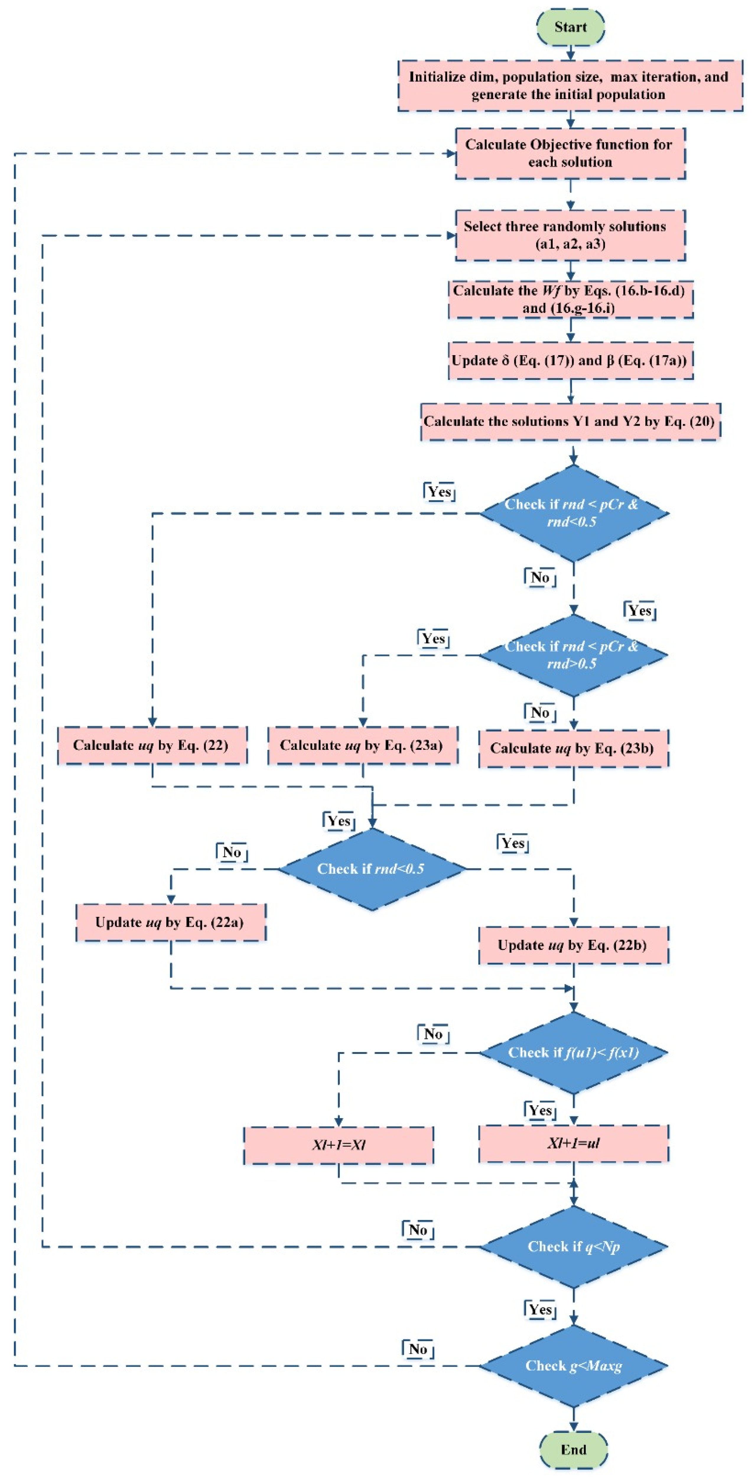
Figure 1 describes the suggested WMV’s flowchart.

4. Simulation Results

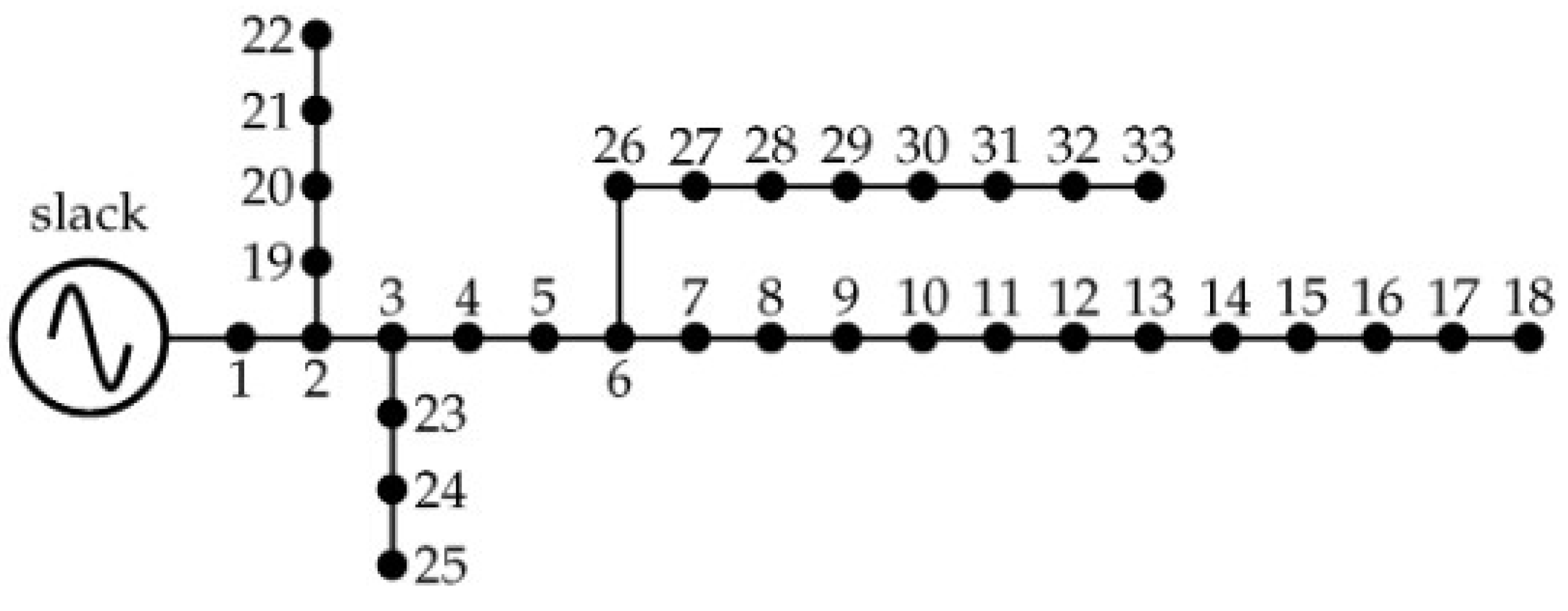
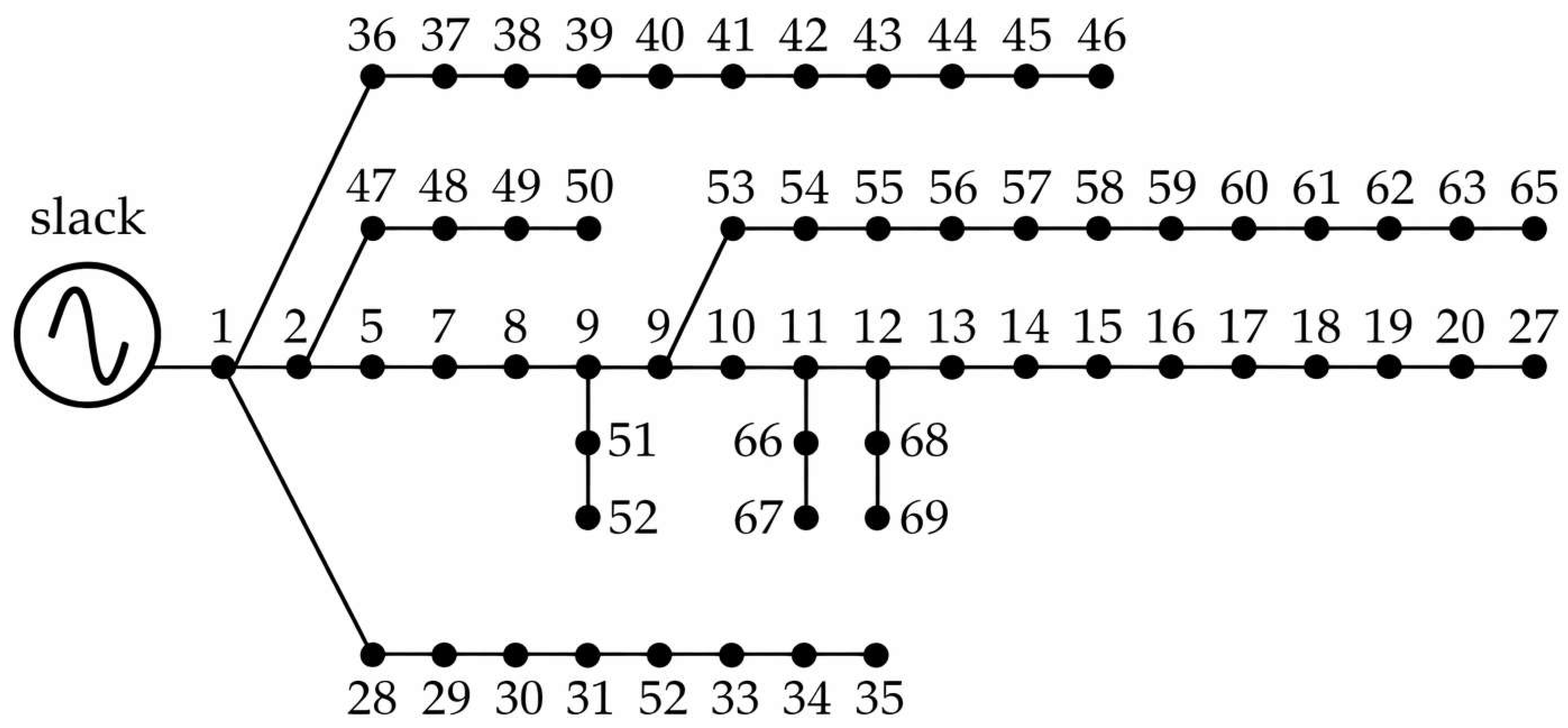
The IEEE 33-node and 69-node distribution feeders are used to validate the suggested WMV. The associated one-line diagram for the first feeder is displayed in Figure 2, where it consists of 32 distribution lines and 33 nodes [38], and demonstrates a typical voltage of 12.6600 kV. For the nominal loading condition, the total active (MW), reactive (MVAr), and apparent loads (MVA) are 3.7150, 2.3000, and 4.3690, respectively [39]. The networked one-line graph of the second feeder with a typical voltage of 12.66 kV can be seen in Figure 3, where it consists of 68 distribution lines and 69 nodes. The two entire system loads are 2.694 MVAr and 3.802 MW, respectively [40]. Furthermore, PV-STATCOM has a maximum reactive power threshold of ±1000 kVAr.

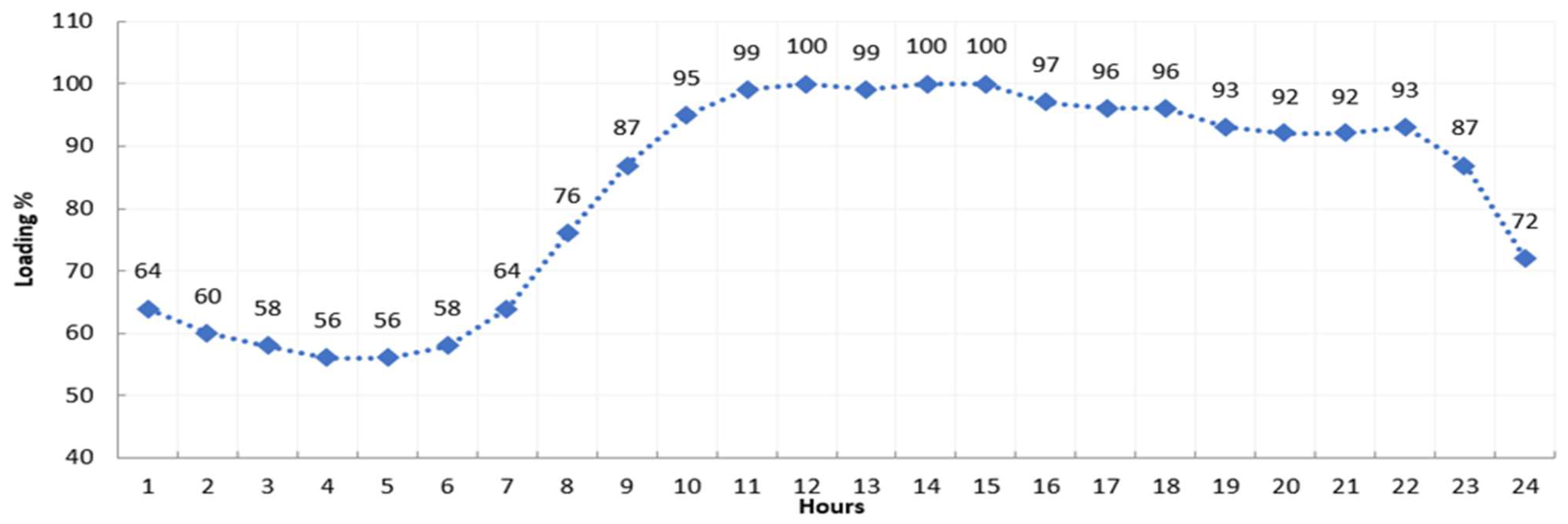
As illustrated in Figure 4 [41], the power factor of each load is maintained constant throughout the simulations, and the distribution nodes are expected to have the same loading curve.

To evaluate the performance of the proposed WMV optimization technique under a controlled and comparable framework, some modeling assumptions are adopted in this study. The hourly load demand is treated as deterministic values representing a typical daily operating scenario as shown in Figure 4. Also, the PV generation profiles are extracted from [42] using the Beta Probability Density Function (PDF) for modeling the uncertainty of solar irradiation hourly. In this form, different solar irradiation conditions are used to develop the Beta-PDF for each hour, and the power output from PV modules is defined for each state of solar irradiation. The reactive power capability of PV inverters is represented in a simplified manner by assuming that PV-STATCOM units can provide reactive power support within predefined limits, without explicitly modeling detailed inverter $P–Q$capability curves. In addition, the study primarily focuses on technical performance indicators, such as energy loss reduction, voltage profile improvement, and network operational feasibility. Therefore, investment costs, installation constraints, and detailed techno-economic analyses are not explicitly incorporated in the optimization model. Furthermore, a constant load power factor is assumed for all buses to maintain consistency with commonly used benchmark models of the IEEE 33-bus and IEEE 69-bus distribution systems.

4.1. Application on IEEE 33-Bus Distribution System

For PV-STATCOM allocation on the first system under examination, the proposed WMV is utilized in contrast to AROA, PSO, GSOA, HPOA and DEA in order to minimize energy losses and compromise voltage variations. There can only be three PV-STATCOM units in total. The results of the WMV, AROA [24], PSO [43], GSOA [24], HPOA [43] and DEA [24] for PV-STATCOM allocation are displayed in

Table 1. Allocations of PV-STATCOM for IEEE 33-distribution feeder.

Items		Initial	Proposed WMV	PSO	HPOA	DEA	GSOA	AROA
PV-STATCOM Devices	Installed nodes	-	30	2	11	10	31	7
		-	13	10	30	32	15	14
		-	29	28	26	33	8	31
	STATCOM Size (kVAr)	-	±892	±1000	±1000	±1000	953	862
		-	±391	±1000	±1000	±1000	965	769
		-	±618	±1000	±1000	±1000	842	838
	PV Size (kW)	-	816	451	840	1000	934	652
		-	999	1000	844	451	448	969
		-	660	1000	767	1000	716	830
$OF$		3557.25	1398.029	2909.081	1534.093	2132.16	2387.5	1643.774
Penalty		-	0	0	0	0	0	0

. In this table, the WMV approach defines the installed buses that have the optimal allocation, where the planned buses are 30, 13, and 29, and their associated PV sizes are 816, 999, and 660 kW, respectively. The accompanying STATCOM sizes at each of the three locations are ±892, ±391, and ±618 kVAr, respectively. According to this data, the suggested WMV reduces energy losses from 3557.25 to 1398.029 with an improvement percentage of 60.69%, resulting in the least amount among other approaches. This improvement in energy losses is percentile evaluated as follows:

$$Improve \%={\displaystyle \frac{OF-{OF}_o}{{OF}_o}}\times 100\%$$

(25)

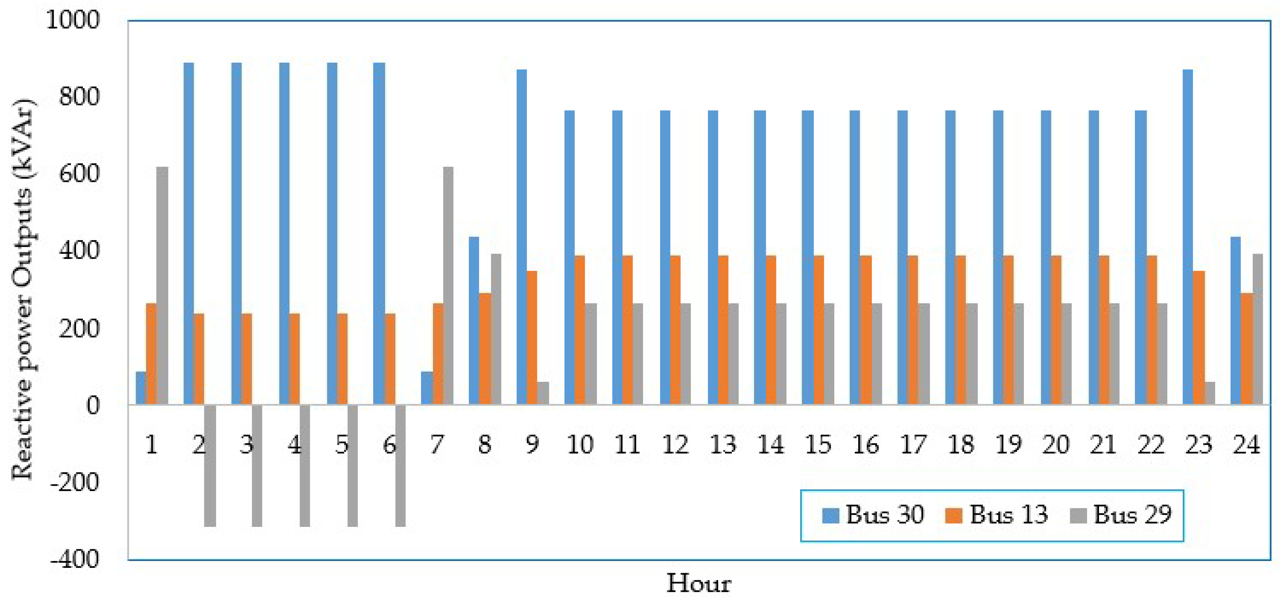
where OF and OF_o are the attained and initial energy losses, respectively. HPOA scores 1534.093 in the second rank; followed by AROA, which scores 1643.77 in the third rank; DEA in fourth place with 2132.16 and GSOA in fifth place with 2387.5. Consequently, PSO has 2909.081, which is the worst objective. Moreover, the hourly reactive power outputs of each PV-STATCOM using the proposed WMV algorithm for the IEEE 33-distribution feeder are manifested in Figure 5.

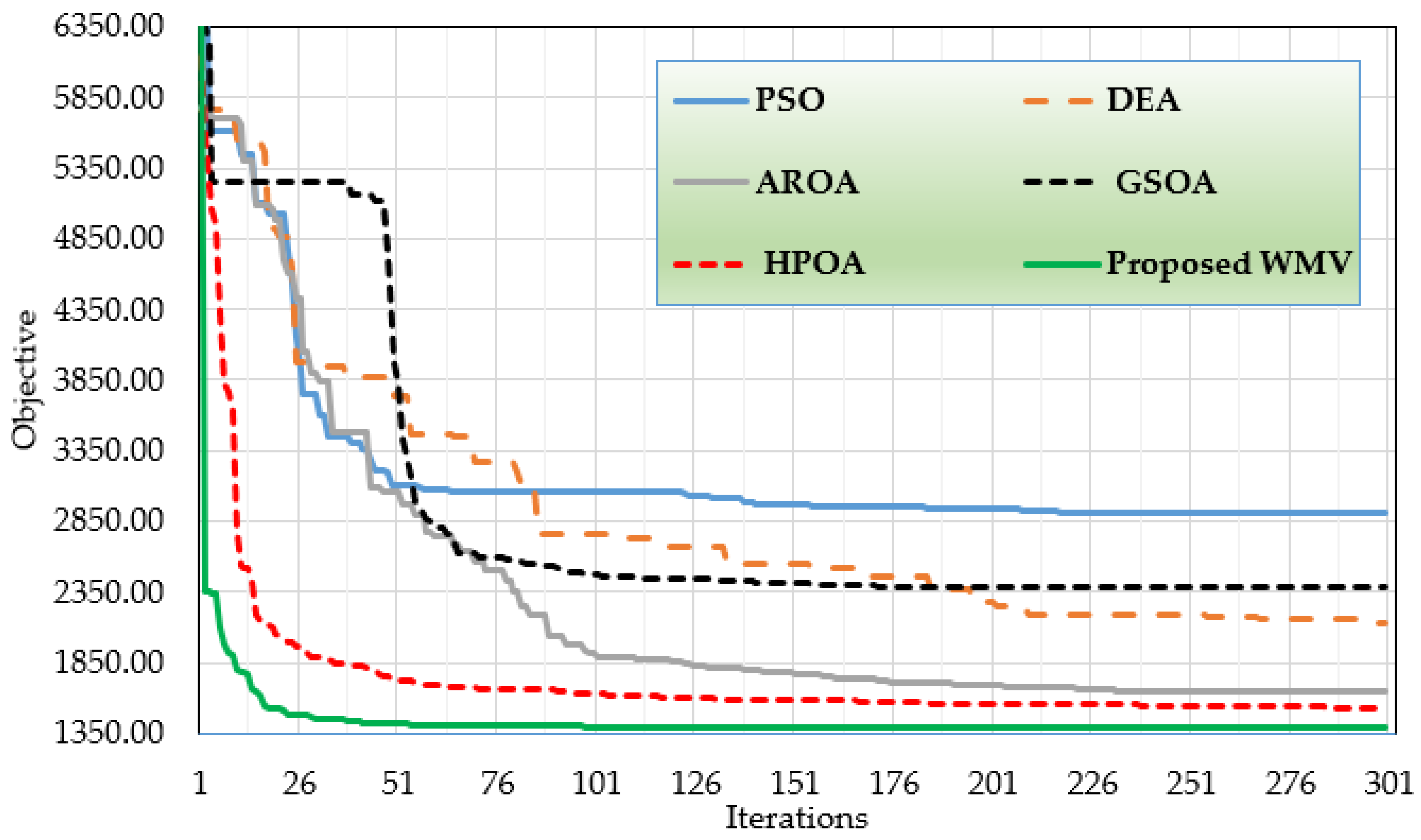
Additionally, the suggested WMV method demonstrates superior convergence features, achieving the lowest trade-off between energy losses and voltage variations compared to other methods, as shown in Figure 6. From the first iterations, WMV approaches lower target values more rapidly.

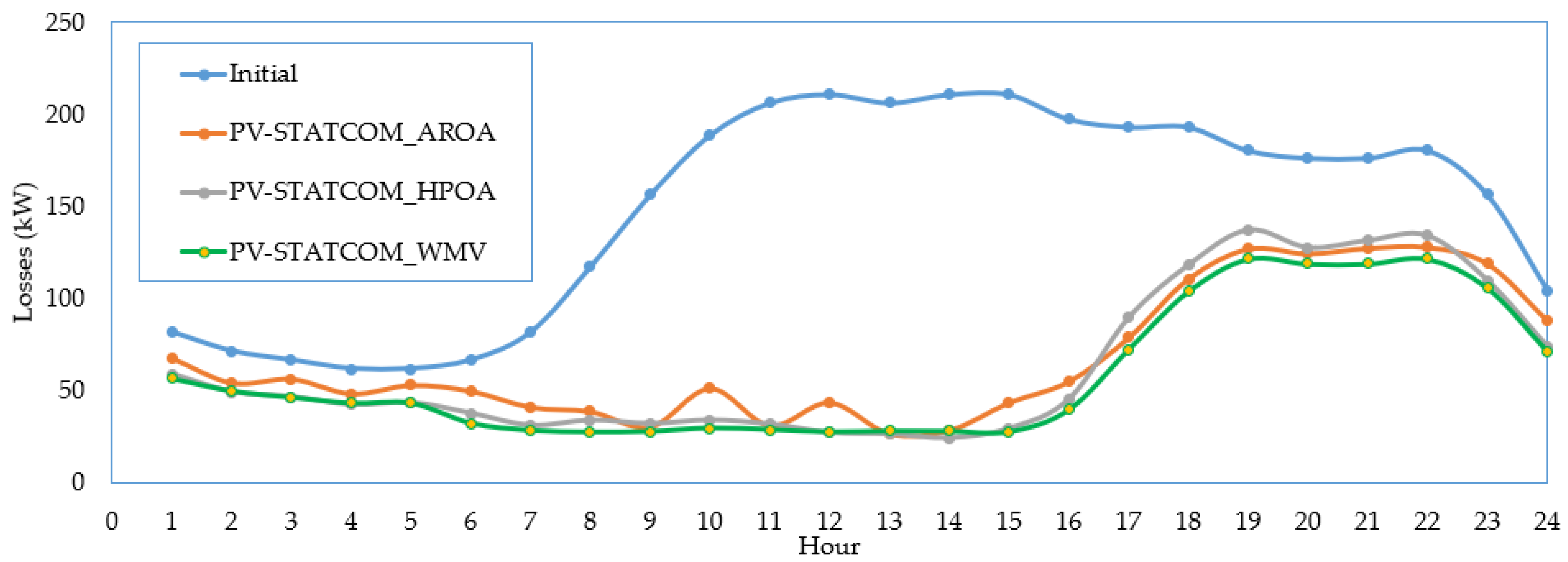
Figure 7 compares the hourly power losses of both of the most effective techniques, WMV and AROA, to the beginning instance in order to better illustrate the differences between them. It is evident that the suggested WMV significantly lowers power losses throughout the day in comparison to the original scenario. In comparison to the initial scenario, the WMV approach significantly reduces the energy losses from 3557.25 kW/day to 1398.0292 kW/day by 60.70%. The energy loss objective is expressed in kW/day, representing the total daily energy losses in the distribution network. When compared to AROA, the suggested WMV exhibits a notable decrease in power losses over the majority of hours. When using the WMV method instead of AROA, the energy losses are reduced by 7.64%, from 1513.697 kW/day to 1398.0292 kW/day. Additionally, when using the WMV approach instead of AROA, the energy losses are reduced by 13.89%, from 1623.5602 kW/day to 1398.0292 kW/day.

Furthermore, in order to quantify the improvements in the voltage profile all over the day, a voltage deviation index (${Voltage}_{Dev}$) is estimated as shown in Equation (26):

$${Voltage}_{Dev}=\sum _{hr=1}^{24}\left(\sum _{k=1}^{N_b}\left|V_k-1\right|\right)$$

(26)

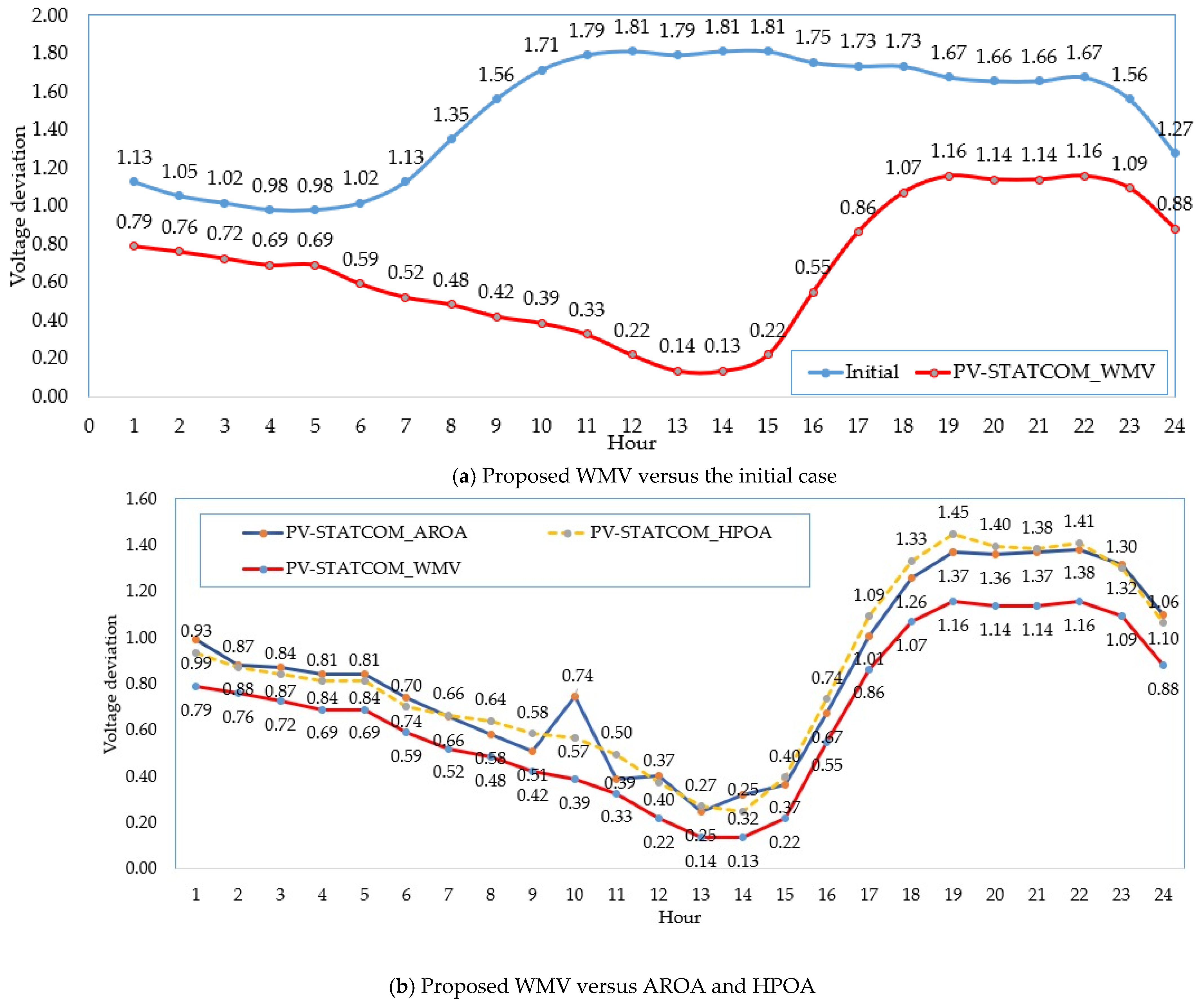
Figure 8 shows the associated hourly voltage deviations of WMV in comparison to AROA, HPOA and the initial scenario. Both AROA and HPOA achieve relatively similar advantages of 20.21 and 20.38 PU/day, respectively. The voltage deviation index is expressed in PU/day, which is a cumulative per-unit voltage deviation measure used to evaluate voltage profile quality across all buses and hours. Applying the WMV method reduces voltage deviations from 35.643 PU/day to 16.13 PU/day, a 54.75% reduction over the initial scenario.

4.2. Application on IEEE 69-Bus Distribution System

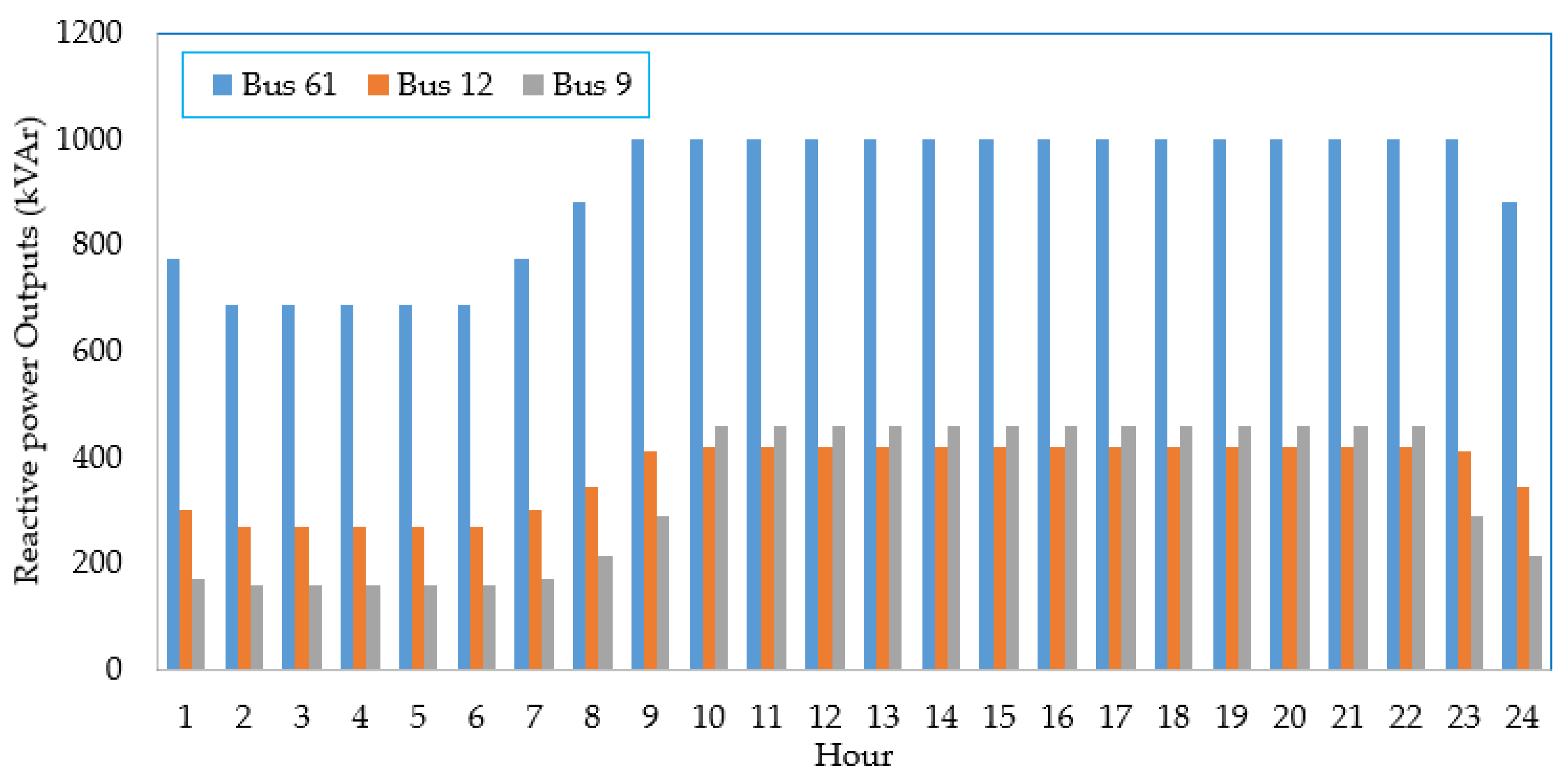
For PV-STATCOM allocation on the second system under examination, the proposed WMV is utilized in contrast to AROA, PSO, GSOA, HPOA and DEA in order to minimize energy losses and compromise voltage variations. There can only be three PV-STATCOM units in total. The results of the WMV, AROA [24], PSO [43], GSOA [24], HPOA [43] and DEA [24] for PV-STATCOM allocation are displayed in

Table 2. PV-STATCOM allocations for IEEE 69-distribution feeder.

Items		Initial	Proposed WMV	PSO	HPOA	DEA	GSOA	AROA
PV-STATCOM Devices	Installed nodes	-	61	63	63	61	64	61
		-	12	62	61	64	59	64
		-	9	61	2	69	62	62
	STATCOM Size (kVAr)	-	±1000	±1000	±1000	±1000	928	957
		-	±420	±1000	±1000	±1000	850	876
		-	±457	±1000	±1000	±1000	937	911
	PV Size (kW)	-	1000	508	1000	1000	967	737
		-	994	1000	1000	1000	488	964
		-	540	1000	10	498	806	774
$OF$		3821.4161	1527.795	2416.336	1616.607	1814.308	1952.972	1622.933
Penalty		-	0	0	0	0	0	0

. In this table, the WMV approach defines the installed buses that have the optimal allocation where the planned buses are 61, 12, and 9, and their associated PV sizes are 1000, 994, and 540 kW, respectively. The accompanying STATCOM sizes at each of the three locations are ±1000, ±420, and ±457 kVAr, respectively. According to this data, the suggested WMV reduces energy losses from 3821.42 to 1527.795 with an improvement percentage of 60.02%, resulting in the least amount among other approaches. HPOA scores 1616.607 in the second rank; followed by AROA, which scores 1622.933 in the third rank; DEA in fourth place with 1814.308 and GSOA in fifth place with 1952.972. Consequently, PSO has 2416.336, which is the worst objective. Moreover, the hourly reactive power outputs of each PV-STATCOM using the proposed WMV algorithm for the IEEE 69-distribution feeder are shown in Figure 9.

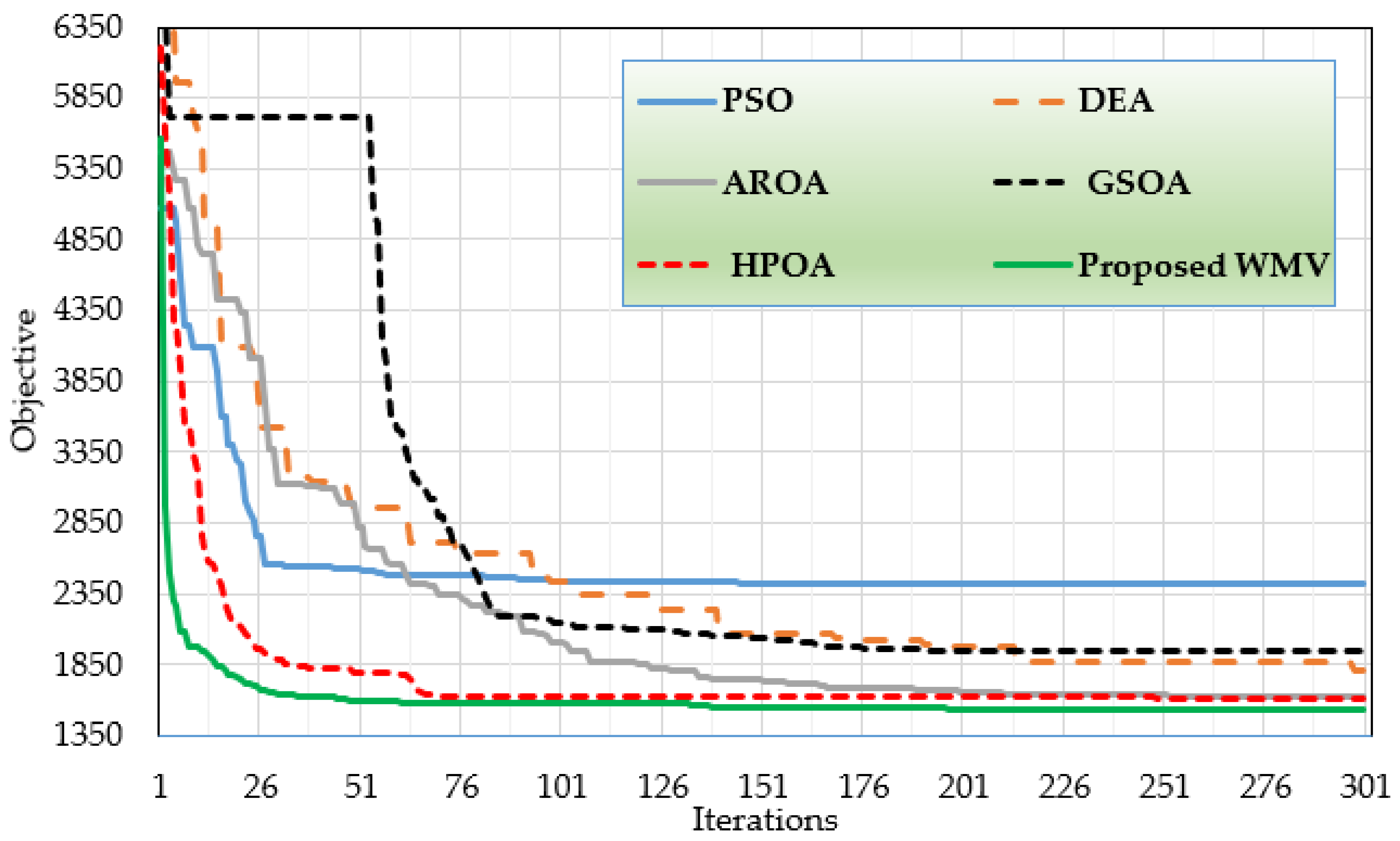
Additionally, their pertinent convergence characteristics are displayed in Figure 10. As demonstrated from this figure, the suggested WMV achieves the lowest trade-off of energy losses and voltage variations as compared to all the other methods used, yielding outstanding convergence features. Beginning in the first iterations, the suggested WMV exhibits a quicker approach to the lower target values.

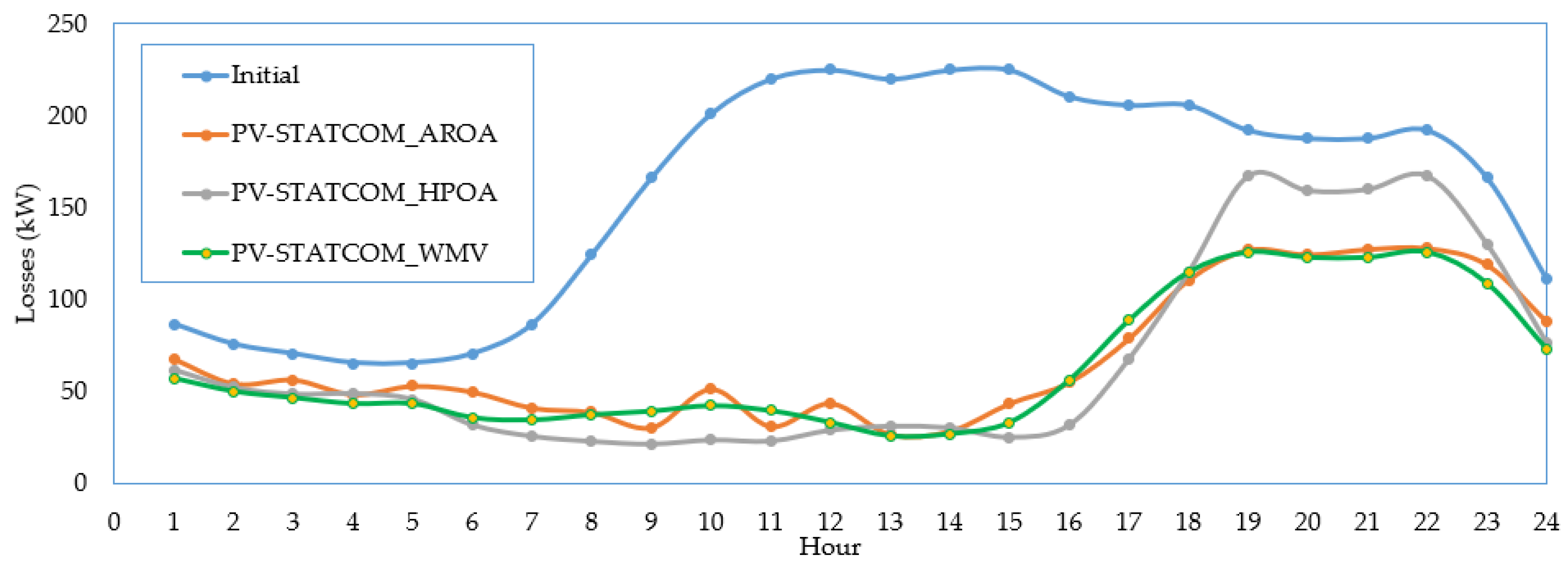
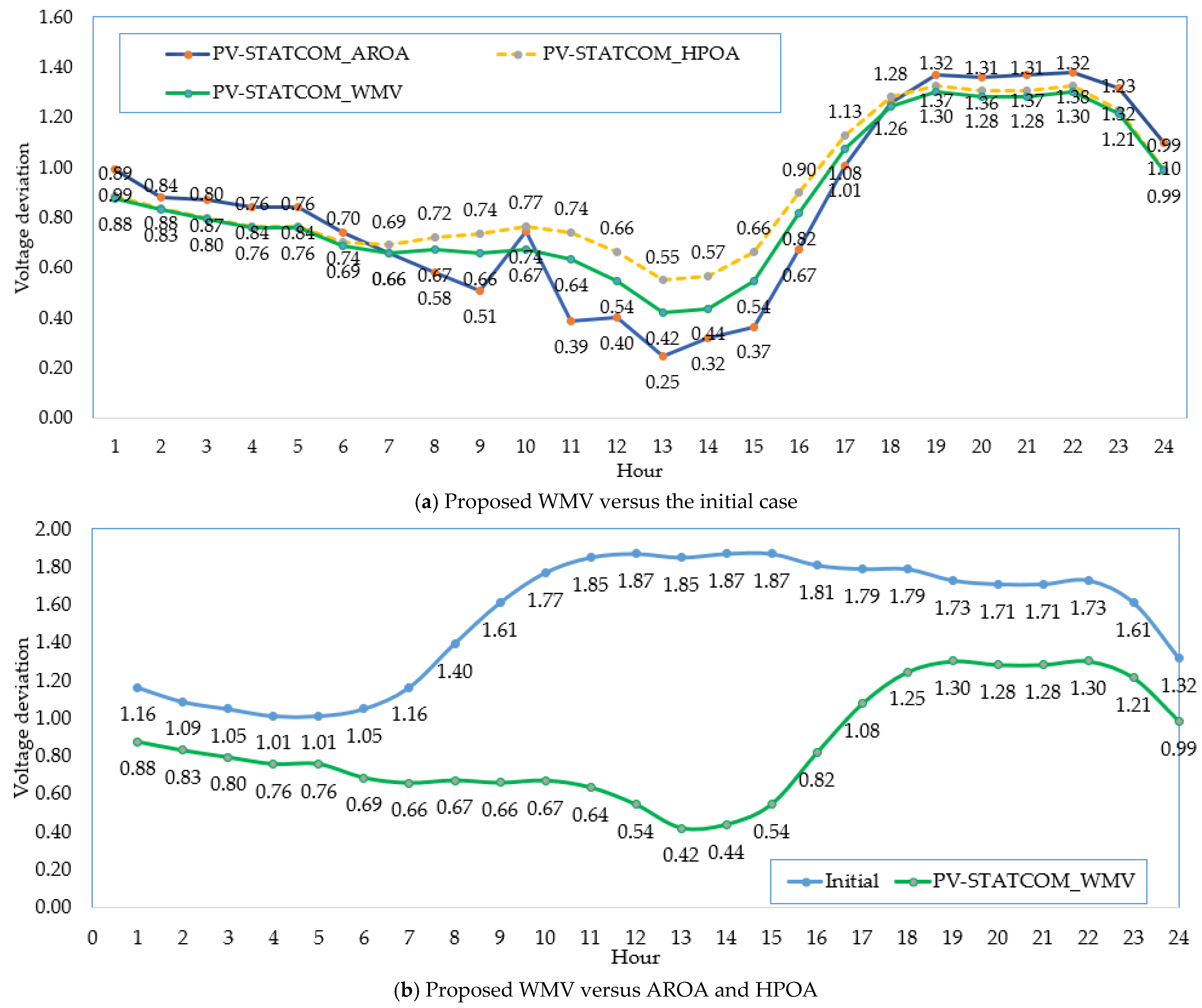
Figure 11 compares the hourly power losses of both of the most effective techniques, WMV and AROA, to the beginning instance in order to better illustrate the differences between them. It is evident that the suggested WMV significantly lowers power losses throughout the day in comparison to the original scenario. In comparison to the initial scenario, the WMV method significantly reduces the energy losses from 3784.5837 kW/day to 1527.7952 kW/day by 60.70%. When compared to AROA, the suggested WMV exhibits a notable decrease in power losses over the majority of hours. When using the WMV approach instead of AROA, the energy losses are reduced by 5.90%, from 1623.5602 kW/day to 1527.7952 kW/day. Additionally, when using the WMV method instead of AROA, the energy losses are reduced by 4.13%, from 1593.6169 kW/day to 1527.7952 kW/day. Furthermore, Figure 12 shows the associated hourly voltage deviations of WMV in comparison to AROA, HPOA and the initial scenario. Both AROA and HPOA achieve relatively similar advantages of 21.65 and 22.99 PU/day, respectively. It can be noticed that applying the WMV approach reduces voltage deviations from 36.832 PU/day to 20.46 PU/day, a 44.54% reduction over the initial scenario.

4.3. Discussions on Constraint Handling Effectiveness and Feasibility Validation

In this study, the operational constraints of the distribution system are handled through a penalty-based reformulation of the optimization objective function. The inequality constraints associated with bus voltage limits, line thermal limits, and renewable penetration levels are incorporated into the objective function through additional penalty terms. In this approach, the penalty component becomes active only when a constraint violation occurs. When such violations appear, the penalty term assumes a very large value, which significantly increases the objective function value and consequently drives the optimizer toward the feasible region of the search space. As a result, infeasible candidate solutions become unattractive to the optimization algorithm and are automatically discarded during the evolutionary selection process.

Within the designed WMV optimization framework, the penalty parameters were deliberately assigned sufficiently large magnitudes to strongly discourage any violation of operational limits during the search process. In the present study, the penalty coefficients are selected as: $K_A=1000$; $K_B=1000$; $K_C=\mathrm{100,000}$; and $K_D=\mathrm{100,000}$. In this work, larger penalty weights were assigned to voltage magnitude violations since maintaining acceptable voltage levels is one of the most critical operational requirements in distribution networks. Voltage constraint violations can lead to power quality issues and equipment malfunction; therefore, strict enforcement of voltage limits is necessary during the optimization process.

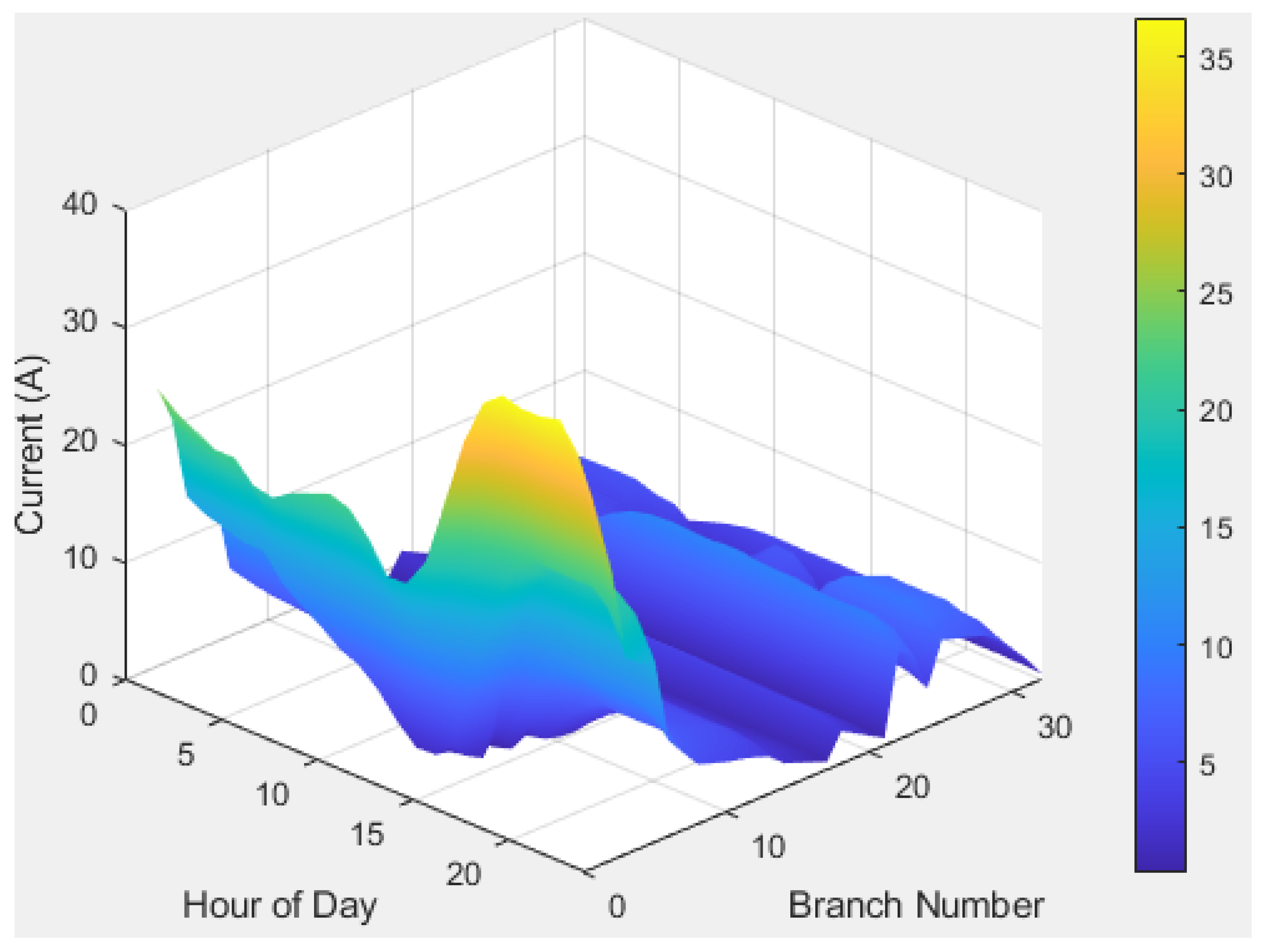
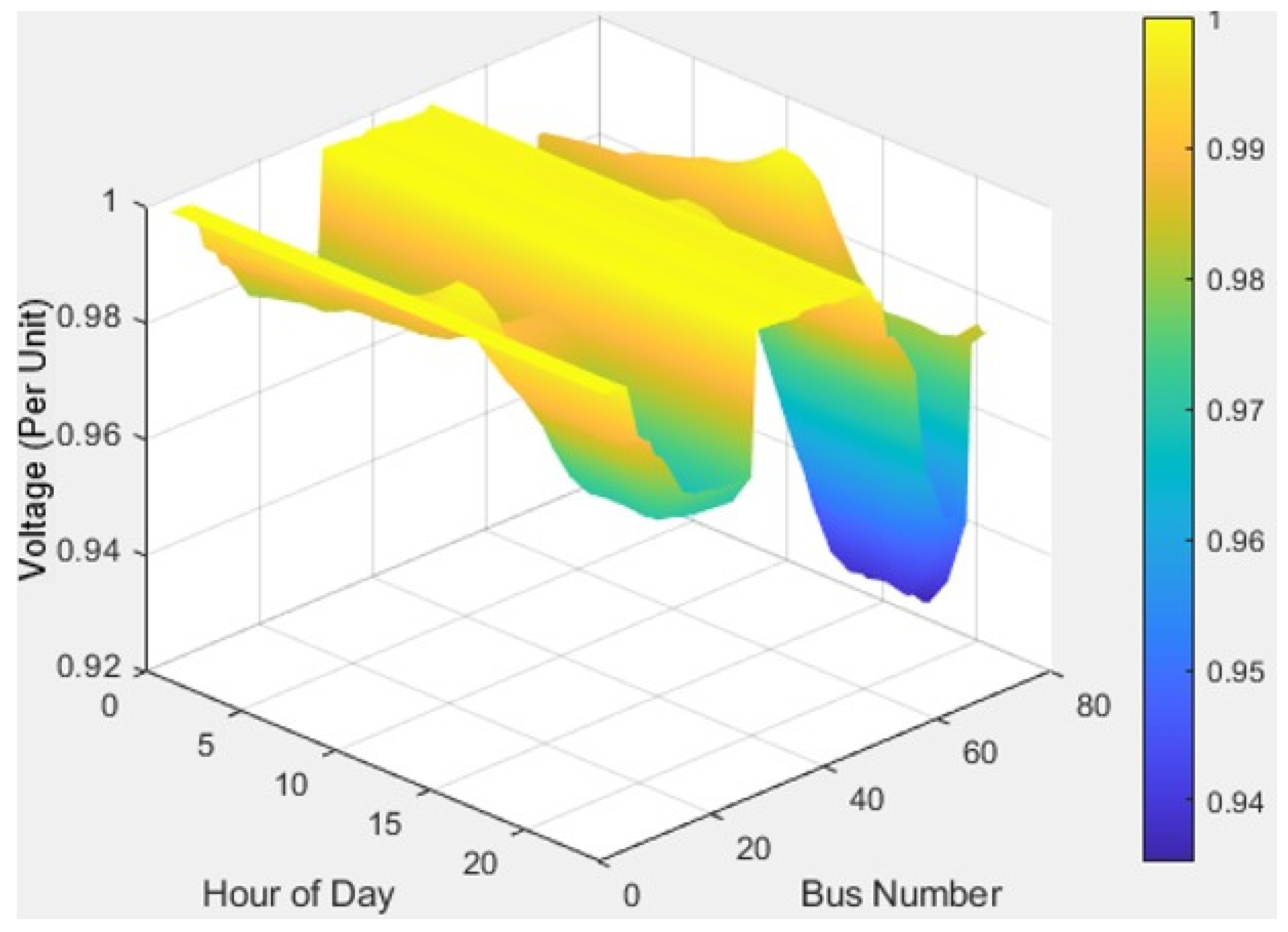
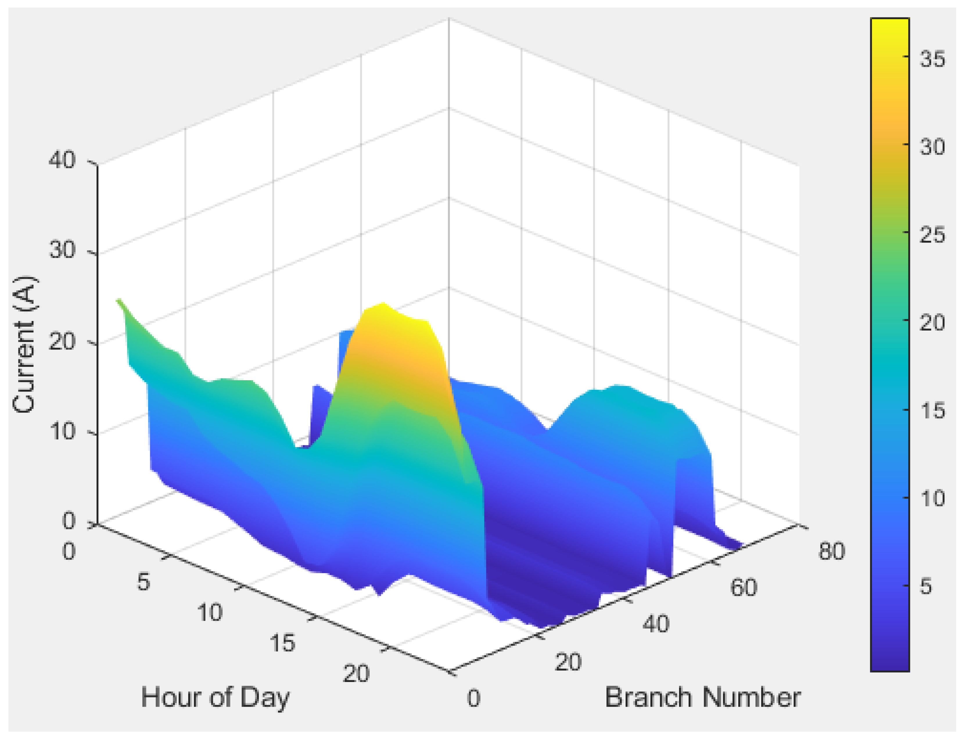
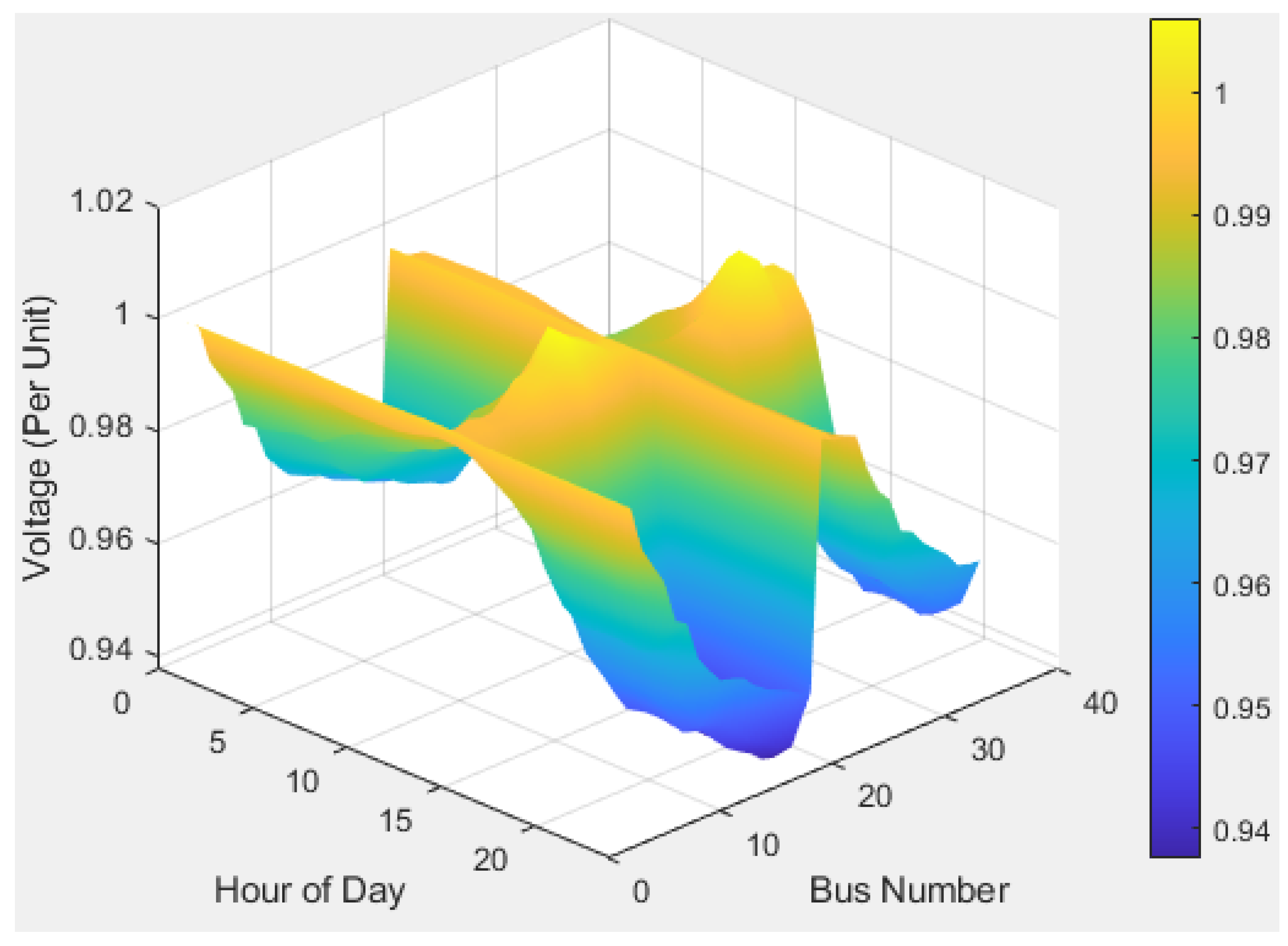
To further validate the effectiveness of the adopted constraint-handling mechanism, three-dimensional (3D) plots of all the bus voltages and branch currents across the 24 h operating horizon are provided in Figure 13, Figure 14, Figure 15 and Figure 16 for both studied systems.

Figure 13 and Figure 14 illustrate the hourly voltage profiles and branch current distributions for the IEEE 33-bus system, respectively. The voltage surface in Figure 13 clearly shows that the voltage magnitudes for all the buses and time intervals remain within the acceptable operational range. Similarly, Figure 14 presents the branch currents across the network, confirming that the thermal limits of all feeders are respected during the entire 24 h operating period.

In addition, Figure 15 and Figure 16 present the same validation analysis for the IEEE 69-bus distribution system. The voltage surface shown in Figure 15 indicates that the proposed optimization framework successfully maintains voltage magnitudes within the allowable range across all the buses and hours. Meanwhile, the branch current distribution illustrated in Figure 16 confirms that line loading remains safely below thermal limits, indicating that no branch overloading occurs in the optimized operating condition.

These plots allow a comprehensive visualization of the system operating conditions and confirm that all the operational constraints are satisfied throughout the entire daily cycle. As shown, all the bus voltages remain within the permissible limits (0.95 p.u.–1.05 p.u.) during all hours of operation. All the branch currents remain below their corresponding thermal capacity limits, ensuring secure line loading conditions.

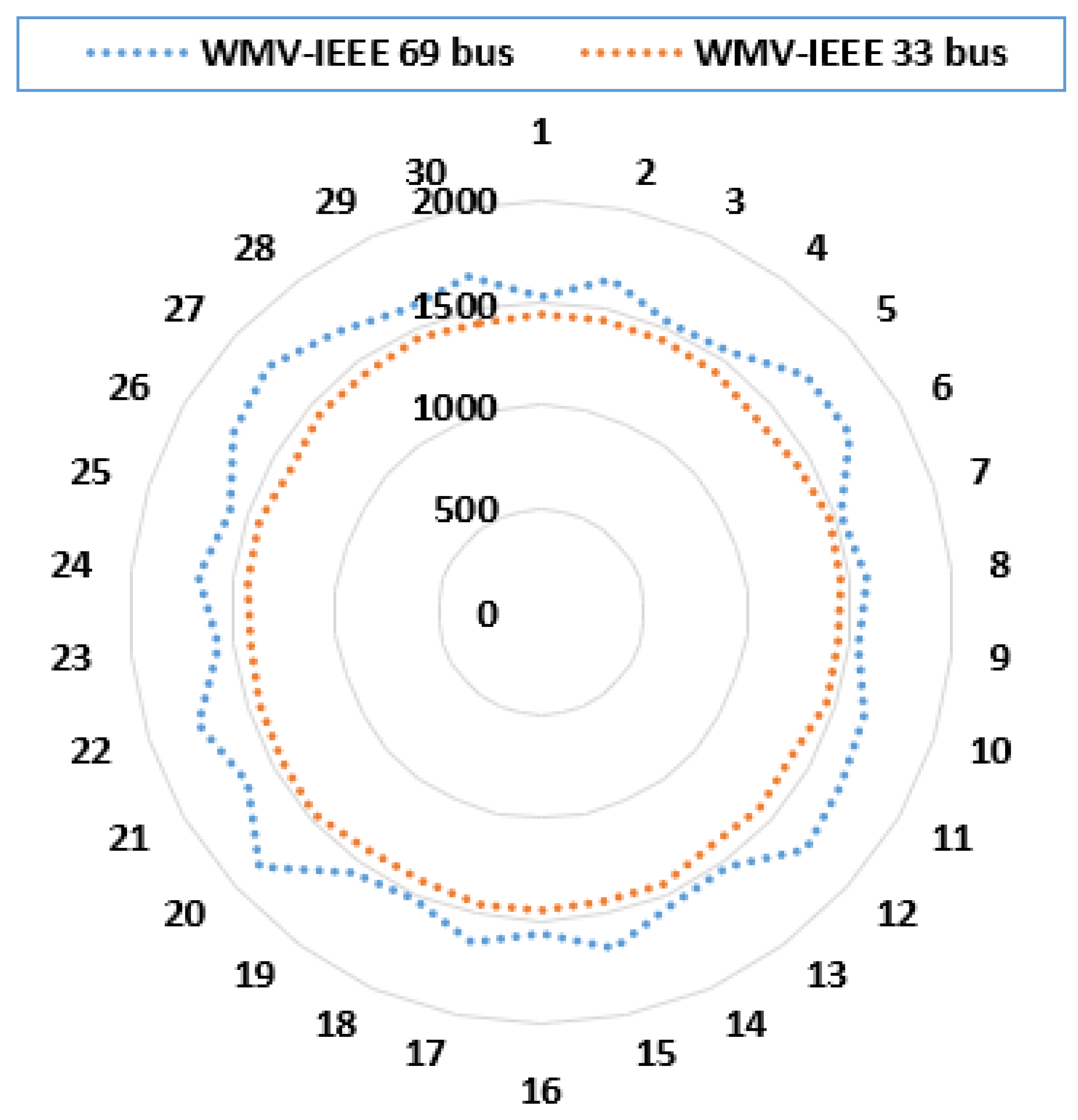
The robustness and stability of the proposed WMV technique were further evaluated by performing thirty independent runs for each test system, and the statistical performance indicators are summarized in Figure 17. The obtained results demonstrate a consistent convergence behavior of the proposed optimizer with limited variability among the independent executions. For the IEEE 69-bus system, the best obtained daily energy loss is 1527.795 kWh, while the average and worst values are 1633.659 kWh and 1840.404 kWh, respectively, with a standard deviation of 85.053. Similarly, for the IEEE 33-bus system, the best energy loss is 1398.029 kWh, while the average and worst values are 1436.724 kWh and 1473.385 kWh, respectively, with a relatively small standard deviation of 18.289. The relatively low dispersion of the obtained solutions, particularly for the IEEE 33-bus system, confirms the high stability and repeatability of the proposed WMV technique, indicating that the algorithm is capable of consistently locating high-quality solutions without significant sensitivity to the stochastic initialization of the population.

In addition to robustness analysis, the computational efficiency of the proposed WMV method was also evaluated and compared with several recently reported optimization techniques, including AROA [24], DEA [24], and GSOA [24], as presented in

Table 3. Average computational times of the AROA [24], DEA [24], and GSOA [24] for the IEEE 33-distribution system.

Items	AROA	DEA	GSOA	Proposed WMV
Computational Time (seconds)	531.833	585.51	758.85	577.21

. The results indicate that the proposed WMV algorithm requires an average computational time of 577.21 s for the IEEE 33-bus distribution system. This value is significantly lower than that of GSOA (758.85 s) and DEA (585.51 s), while remaining comparable to AROA (531.833 s).

5. Conclusions

This paper presented a constrained mathematical optimization framework for the optimal allocation and sizing of PV-STATCOM devices in radial distribution systems under 24 h load variations. The problem was formulated as a nonlinear, non-convex optimization model aiming to simultaneously minimize daily energy losses while satisfying operational constraints, including voltage magnitude limits, branch thermal capacities, inverter active/reactive power limits, and renewable penetration restrictions. A penalty-based reformulation was adopted to effectively incorporate inequality constraints into the objective function. To solve the resulting optimization problem, the weighted mean of vectors (WMV) algorithm was employed. The WMV optimizer integrates a wavelet-based weighted mean mechanism, a mean-driven rule update strategy, a vector combining operator to enhance population diversity, and a local search refinement process to improve convergence accuracy. This hybrid structure enables a balanced trade-off between global exploration and local exploitation within complex feasible search domains typical of power system planning problems.

The proposed mathematical framework was validated on the IEEE 33-bus and IEEE 69-bus distribution systems considering realistic daily loading profiles. The simulation results demonstrated substantial reductions in daily energy losses compared to the initial operating conditions. Moreover, when benchmarked against established metaheuristic approaches, including PSO, DEA, AROA, and GSOA, the WMV algorithm consistently achieved superior compromise solutions with improved convergence characteristics and enhanced robustness. The analysis also confirmed that the appropriate placement and sizing of multiple PV-STATCOM units significantly improve voltage regulation and system efficiency across all hourly operating conditions, maintaining voltage magnitudes within acceptable limits throughout the day.

Future work may extend the proposed formulation by incorporating stochastic modeling of solar generation uncertainty, investment cost considerations for techno-economic planning, multi-objective Pareto-based optimization, power reserve optimization [44] and hybridization of WMV with deterministic mathematical programming techniques. Additionally, integrating probabilistic load modeling and inverter capability curves could enhance practical applicability in real-world smart grid environments.

References

1. Fernández, G.; Martínez, A.; Galán, N.; Ballestín-Fuertes, J.; Muñoz-Cruzado-Alba, J.; López, P.; Stukelj, S.; Daridou, E.; Rezzonico, A.; Ioannidis, D. Optimal d-statcom placement tool for low voltage grids. Energies 2021, 14, 4212. [Google Scholar] [CrossRef] [Scilit]
2. Alves, Z.M.; Martins, R.M.; Marchesan, G.; Junior, G.C. Metaheuristic for the Allocation and Sizing of PV-STATCOMs for Ancillary Service Provision. Energies 2022, 16, 424. [Google Scholar] [CrossRef] [Scilit]
3. Luo, L.; Gu, W.; Zhang, X.-P.; Cao, G.; Wang, W.; Zhu, G.; You, D.; Wu, Z. Optimal siting and sizing of distributed generation in distribution systems with PV solar farm utilized as STATCOM (PV-STATCOM). Appl. Energy 2018, 210, 1092–1100. [Google Scholar] [CrossRef] [Scilit]
4. Molzahn, D.K.; Hiskens, I.A. A Survey of Relaxations and Approximations of the Power Flow Equations. Found. Trends Electr. Energy Syst. 2019, 4, 1–221. [Google Scholar] [CrossRef] [Scilit]
5. Yang, C.; Sun, Y.; Zou, Y.; Zheng, F.; Liu, S.; Zhao, B.; Wu, M.; Cui, H. Optimal Power Flow in Distribution Network: A Review on Problem Formulation and Optimization Methods. Energies 2023, 16, 5974. [Google Scholar] [CrossRef] [Scilit]
6. Wang, C.; Luo, F.; Jiao, Z.; Zhang, X.; Lu, Z.; Wang, Y.; Zhao, R.; Yang, Y. An Enhanced Second-Order Cone Programming-Based Evaluation Method on Maximum Hosting Capacity of Solar Energy in Distribution Systems with Integrated Energy. Energies 2022, 15, 9025. [Google Scholar] [CrossRef] [Scilit]
7. Li, Q.; Ayyanar, R.; Vittal, V. Convex optimization for des planning and operation in radial distribution systems with high penetration of photovoltaic resources. IEEE Trans. Sustain. Energy 2016, 7, 985–995. [Google Scholar] [CrossRef] [Scilit]
8. Chowdhury, M.M.U.T.; Kamalasadan, S. An Angle Included Optimal Power Flow (OPF) Model for Power Distribution Network Using Second Order Cone Programming (SOCP). In Proceedings of the 2020 IEEE Industry Applications Society Annual Meeting, IAS 2020, Detroit, MI, USA, 10–16 October 2020. [Google Scholar] [CrossRef] [Scilit]
9. Gil-González, W.; Molina-Cabrera, A.; Montoya, O.D.; Grisales-Noreña, L.F. An mi-sdp model for optimal location and sizing of distributed generators in dc grids that guarantees the global optimum. Appl. Sci. 2020, 10, 7681. [Google Scholar] [CrossRef] [Scilit]
10. Alqahtani, M.H.; Ginidi, A.R.; Aljumah, A.S.; Shaheen, A.M. Cost-Effective and Low-Carbon Emission Deployment of PV-DG Integration in Distribution Networks Using Self-Adaptive Bonobo Optimizer. Int. J. Energy Res. 2025, 2025, 8830028. [Google Scholar] [CrossRef] [Scilit]
11. El-Rifaie, A.M.; Shaheen, A.M.; Tolba, M.A.; Smaili, I.H.; Moustafa, G.; Ginidi, A.R.; Elshahed, M.A. Modified Gradient-Based Algorithm for Distributed Generation and Capacitors Integration in Radial Distribution Networks. IEEE Access 2023, 11, 120899–120917. [Google Scholar] [CrossRef] [Scilit]
12. Moustafa, G.; Tolba, M.A.; El-Rifaie, A.M.; Ginidi, A.; Shaheen, A.M.; Abid, S. A Subtraction-Average-Based Optimizer for Solving Engineering Problems with Applications on TCSC Allocation in Power Systems. Biomimetics 2023, 8, 332. [Google Scholar] [CrossRef] [Scilit] [PubMed]
13. Shriya, U.; Veena, S.H. Increasing Grid Power Transmission Using PV-STATCOM. In Proceedings of the 2021 6th International Conference for Convergence in Technology, I2CT 2021, Maharashtra, India, 2–4 April 2021. [Google Scholar] [CrossRef] [Scilit]
14. Aljumah, A.S.; Alqahtani, M.H.; Shaheen, A.M.; Ginidi, A.R. Adaptive operational allocation of D-SVCs in distribution feeders using modified artificial rabbits algorithm. Electr. Power Syst. Res. 2025, 245, 111588. [Google Scholar] [CrossRef] [Scilit]
15. Aljumah, A.S.; Alqahtani, M.H.; Ginidi, A.R.; Shaheen, A.M. Improved Artificial Hummingbird Algorithm for Optimal Allocation of SVCs in Distribution Networks to Maximize Energy Efficiency. J. Mod. Power Syst. Clean Energy 2026, 14, 261–272. [Google Scholar] [CrossRef] [Scilit]
16. Alqahtani, M.H.; Almutairi, S.Z.; Aljumah, A.S.; Ginidi, A.R.; Shaheen, A.M. Enhanced power grid performance through Gorilla Troops Algorithm-guided thyristor controlled series capacitors allocation. Heliyon 2024, 10, e34326. [Google Scholar] [CrossRef] [Scilit]
17. Sirjani, R. Optimal Placement and Sizing of PV-STATCOM in Power Systems Using Empirical Data and Adaptive Particle Swarm Optimization. Sustainability 2018, 10, 727. [Google Scholar] [CrossRef] [Scilit]
18. Varma, R.K.; Khadkikar, V.; Seethapathy, R. Nighttime application of PV solar farm as STATCOM to regulate grid voltage. IEEE Trans. Energy Convers. 2009, 24, 983–985. [Google Scholar] [CrossRef] [Scilit]
19. Varma, R.K.; Das, B.; Axente, I.; Vanderheide, T. Optimal 24-hr utilization of a PV solar system as STATCOM (PV-STATCOM) in a distribution network. In Proceedings of the IEEE Power and Energy Society General Meeting, Detroit, MI, USA, 24–28 July 2011. [Google Scholar] [CrossRef] [Scilit]
20. Gasperic, S.; Mihalic, R. Estimation of the efficiency of FACTS devices for voltage-stability enhancement with PV area criteria. Renew. Sustain. Energy Rev. 2019, 105, 144–156. [Google Scholar] [CrossRef] [Scilit]
21. Sadiq, R.; Wang, Z.; Chung, C.Y.; Zhou, C.; Wang, C. A review of STATCOM control for stability enhancement of power systems with wind/PV penetration: Existing research and future scope. Int. Trans. Electr. Energy Syst. 2021, 31, e13079. [Google Scholar] [CrossRef] [Scilit]
22. Varma, R.K.; Siavashi, E.M. Enhancement of solar farm connectivity with smart PV inverter PV-STATCOM. IEEE Trans. Sustain. Energy 2019, 10, 1161–1171. [Google Scholar] [CrossRef] [Scilit]
23. Varma, R.K.; Siavashi, E.M. PV-STATCOM: A New Smart Inverter for Voltage Control in Distribution Systems. IEEE Trans. Sustain. Energy 2018, 9, 1681–1691. [Google Scholar] [CrossRef] [Scilit]
24. Elshahed, M.; Tolba, M.A.; El-Rifaie, A.M.; Ginidi, A.; Shaheen, A.; Mohamed, S.A. An Artificial Rabbits’ Optimization to Allocate PVSTATCOM for Ancillary Service Provision in Distribution Systems. Mathematics 2023, 11, 339. [Google Scholar] [CrossRef] [Scilit]
25. Kumar, P.; Bohre, A.K. Optimal allocation of Hybrid Solar-PV with STATCOM based on Multi-objective Functions using combined OPF-PSO Method. In Proceedings of the International Conference on IoT Based Control Networks & Intelligent Systems – ICICNIS, Online, 28–29 June 2021. [Google Scholar] [CrossRef] [Scilit]
26. Popavath, L.N.; Kaliannan, P. Photovoltaic-STATCOM with low voltage ride through strategy and power quality enhancement in a grid integrated Wind-PV system. Electronics 2018, 7, 51. [Google Scholar] [CrossRef] [Scilit]
27. Ahmadianfar, I.; Heidari, A.A.; Noshadian, S.; Chen, H.; Gandomi, A.H. INFO: An efficient optimization algorithm based on weighted mean of vectors. Expert Syst. Appl. 2022, 195, 116516. [Google Scholar] [CrossRef] [Scilit]
28. Elnagi, M.; Kamel, S.; Ramadan, A.; Elnaggar, M.F. Photovoltaic Models Parameters Estimation Based on Weighted Mean of Vectors. Comput. Mater. Contin. 2023, 74, 5229–5250. [Google Scholar] [CrossRef] [Scilit]
29. Ikram, R.M.A.; Mostafa, R.R.; Chen, Z.; Parmar, K.S.; Kisi, O.; Zounemat-Kermani, M. Water Temperature Prediction Using Improved Deep Learning Methods through Reptile Search Algorithm and Weighted Mean of Vectors Optimizer. J. Mar. Sci. Eng. 2023, 11, 259. [Google Scholar] [CrossRef] [Scilit]
30. Tang, X.; Zhang, H.; Taheri, B. Opimal design and 4E evaluation of a CCHP system using an improved version of weighted mean of vectors algorithm. Int. J. Hydrogen Energy 2023, 48, 16457–16469. [Google Scholar] [CrossRef] [Scilit]
31. Nasef, A.; Shaheen, A.; Khattab, H. Local and remote control of automatic voltage regulators in distribution networks with different variations and uncertainties: Practical cases study. Electr. Power Syst. Res. 2022, 205, 107773. [Google Scholar] [CrossRef] [Scilit]
32. Shaheen, A.M.; Alassaf, A.; Alsaleh, I.; Elsayed, A.M. Enhanced Kepler optimization for efficient penetration of PV sources integrated with STATCOM devices in power distribution systems. Expert Syst. Appl. 2024, 253, 124333. [Google Scholar] [CrossRef] [Scilit]
33. Shaheen, A.M.; Elsayed, A.M.; El-Sehiemy, R.A.; Kamel, S.; Ghoneim, S.S.M. A modified marine predators optimization algorithm for simultaneous network reconfiguration and distributed generator allocation in distribution systems under different loading conditions. Eng. Optim. 2021, 54, 687–708. [Google Scholar] [CrossRef] [Scilit]
34. Shaheen, A.; Elsayed, A.; Ginidi, A.; El-Sehiemy, R.; Elattar, E. Reconfiguration of electrical distribution network-based DG and capacitors allocations using artificial ecosystem optimizer: Practical case study. Alex. Eng. J. 2022, 61, 6105–6118. [Google Scholar] [CrossRef] [Scilit]
35. Shaheen, A.M.; Elsayed, A.M.; Ginidi, A.R.; El-Sehiemy, R.A.; Elattar, E.E. Improved Heap-Based Optimizer for DG Allocation in Reconfigured Radial Feeder Distribution Systems. IEEE Syst. J. 2022, 16, 6371–6380. [Google Scholar] [CrossRef] [Scilit]
36. Alqahtani, M.H.; Draz, A.; Shaheen, A.M.; El-Fergany, A.A. Advanced Relay Coordination in Power Networks Considering Transformer Inrush and Motor Starting Currents via Weighted Mean Variance Optimizer. IEEE Access 2024, 12, 184953–184975. [Google Scholar] [CrossRef] [Scilit]
37. Shaheen, A.M.; El-Rifaie, A.M.; Al Faiya, B.; Moustafa, G.; Alnami, H. Economic and environmental optimization-dispatch in large-scale power systems using weighted mean of vectors algorithm. Sustain. Comput. Inform. Syst. 2025, 48, 101265. [Google Scholar] [CrossRef] [Scilit]
38. Khattab, H.A.; Aljumah, A.S.; Shaheen, A.M.; Omar, H.A. Improved Manta Ray Foraging Algorithm for Optimal Allocation Strategies to Power Delivery Capabilities in Active Distribution Networks. IEEE Access 2024, 12, 157699–157715. [Google Scholar] [CrossRef] [Scilit]
39. Shaheen, A.; El-Sehiemy, R.; Kamel, S.; Selim, A. Optimal Operational Reliability and Reconfiguration of Electrical Distribution Network Based on Jellyfish Search Algorithm. Energies 2022, 15, 6994. [Google Scholar] [CrossRef] [Scilit]
40. Paz-Rodríguez, A.; Castro-Ordoñez, J.F.; Montoya, O.D.; Giral-Ramírez, D.A. Optimal integration of photovoltaic sources in distribution networks for daily energy losses minimization using the vortex search algorithm. Appl. Sci. 2021, 11, 4418. [Google Scholar] [CrossRef] [Scilit]
41. El-Ela, A.; El-Sehiemy, R.A.; Allam, S.M.; Shaheen, A.M.; Nagem, N.A.; Sharaf, A.M. Renewable Energy Micro-Grid Interfacing: Economic and Environmental Issues. Electronics 2022, 11, 815. [Google Scholar] [CrossRef] [Scilit]
42. Shaheen, A.M.; Elattar, E.E.; Nagem, N.A.; Nasef, A.F. Allocation of PV Systems with Volt/Var Control Based on Automatic Voltage Regulators in Active Distribution Networks. Sustainability 2023, 15, 15634. [Google Scholar] [CrossRef] [Scilit]
43. Shaheen, A.M.; El-Sehiemy, R.A.; Ginidi, A.; Elsayed, A.M.; Al-Gahtani, S.F. Optimal Allocation of PV-STATCOM Devices in Distribution Systems for Energy Losses Minimization and Voltage Profile Improvement via Hunter-Prey-Based Algorithm. Energies 2023, 16, 2790. [Google Scholar] [CrossRef] [Scilit]
44. Aljumah, A.S.; Alqahtani, M.H.; Ginidi, A.R.; Shaheen, A.M. Combined heat and power dispatch with reserve constraints using a mutated trochoid searching optimizer. Electr. Power Syst. Res. 2026, 252, 112447. [Google Scholar] [CrossRef] [Scilit]
Figure 1. Main steps of the proposed WMV.
Mathematics 14 01351 g001
Figure 2. IEEE 33-distribution feeder.
Mathematics 14 01351 g002
Figure 3. IEEE 69-distribution feeder.
Mathematics 14 01351 g003
Figure 4. Hourly loading profile expressed as a percentage of the nominal state.
Mathematics 14 01351 g004
Figure 5. Hourly reactive power outputs of each PV-STATCOM using the proposed WMV algorithm for the IEEE 33-distribution feeder.
Mathematics 14 01351 g005
Figure 6. Convergence characteristics of the IEEE 33-distribution feeder applied techniques.
Mathematics 14 01351 g006
Figure 7. Hourly power losses based on the proposed WMV, AROA and HPOA versus the initial case for the IEEE 33-distribution feeder.
Mathematics 14 01351 g007
Figure 8. Hourly voltage deviations of the IEEE 33-distribution feeder based on the proposed WMV against the initial case, AROA and HPOA.
Mathematics 14 01351 g008
Figure 9. Hourly reactive power outputs of each PV-STATCOM using the proposed WMV algorithm for the IEEE 69-distribution feeder.
Mathematics 14 01351 g009
Figure 10. Convergence properties of the applied algorithms for the IEEE 69-distribution feeder.
Mathematics 14 01351 g010
Figure 11. Hourly power losses of the IEEE 69-distribution feeder based on the proposed WMV against the initial case, AROA, and HPOA.
Mathematics 14 01351 g011
Figure 12. Hourly voltage deviations of the IEEE 69-distribution feeder based on the proposed WMV against the initial case, AROA and HPOA.
Mathematics 14 01351 g012
Figure 13. All the bus voltages in every hour for the IEEE 33-bus system.
Mathematics 14 01351 g013
Figure 14. All the branch currents in every hour for the IEEE 33-bus system.
Mathematics 14 01351 g014
Figure 15. All the bus voltages in every hour for the IEEE 69-bus system.
Mathematics 14 01351 g015
Figure 16. All the branch currents in every hour for the IEEE 69-bus system.
Mathematics 14 01351 g016
Figure 17. Thirty disparate implementations of the proposed WMV technique for both systems.
Mathematics 14 01351 g017