Stability Test for Multiplicity of Solutions in Finite Element Analysis of Cracking Structures

Abstract

Quasi-brittle structures modeled with softening constitutive laws may lose the uniqueness of equilibrium, producing bifurcation and multiple admissible crack evolutions even under symmetric loading. This paper develops a stability test and a constructive multiplicity procedure for finite element cracking analyses formulated as a Parametric Linear Complementarity Problem (PLCP) solved in tableau form. The approach exploits the pivot sequence of a complementary tableau to monitor stability by tracking the positive definiteness of the reduced active-mode Hessian $\widehat{\mathbf{A}}$ through a complement condition, without eigenvalue computations. A direct relationship between loss of positive definiteness and the sign of the incremental load factor $\Delta \dot{\mathsf{\alpha }}$ is established, providing an intrinsic indicator of transition to descending response. When degeneracy occurs, a “void pivot” mechanism is introduced to generate an alternative admissible tableau, enabling a systematic construction of multiple isolated solutions associated with competing crack patterns. The method is demonstrated on a two-notched direct tension specimen with cohesive softening, where symmetric and antisymmetric paths emerge at a critical step. The implementation is compatible with parallelized matrix operations and remains effective in the presence of non-holonomic constraints.

1. Introduction

In structural engineering computational practice, bifurcation phenomena are generally not treated explicitly and continue to represent an open problem in numerical simulation. In most commercial finite element codes, the possible loss of uniqueness of equilibrium is avoided rather than analyzed, by means of algorithmic strategies primarily introduced to ensure convergence [1]. These include solution procedures that implicitly enforce a single equilibrium path, numerical regularization techniques, or the introduction of artificial imperfections. While effective from a numerical point of view, such strategies tend to bypass the intrinsic multiplicity of admissible solutions.

In contrast to this numerical treatment, structural systems made of quasi-brittle materials such as concrete and masonry exhibit nonlinear responses governed by fracture localization, damage evolution, and progressive stiffness degradation [2]. A well-documented phenomenon in these systems is the emergence of asymmetric crack patterns under perfectly symmetric loading and boundary conditions, which reflects a fundamental loss of uniqueness in equilibrium. In mechanical terms, this behavior is associated with bifurcation and post-critical evolution, where multiple equilibrium branches may satisfy the governing equations simultaneously [3,4].

The assessment of stability and the identification of multiple potential solutions are critical from an engineering perspective. In quasi-brittle materials, a structure might follow a stable symmetric path or a lower-energy asymmetric path; identifying these allows engineers to establish a ranking of different loading-unloading paths in terms of structural safety.

In the context of structural safety, the employment of advanced numerical simulations for stability analysis offers significant advantages over purely empirical or simplified analytical methods. As highlighted in recent literature [5], simulation-based approaches provide a comprehensive framework to explore the entire evolution of failure mechanisms, allowing for a proactive assessment of potential bifurcation points and stability of equilibrium paths. This predictive capability is essential for establishing safety margins in complex cracking structures, as it enables a rigorous investigation into how small perturbations or material heterogeneities may trigger sudden changes in the structural response, ultimately leading to more robust and reliable design strategies.

From a computational standpoint, capturing these competing branches is essential for structural safety assessment because different admissible crack paths can entail markedly different load capacities, deformation states, and collapse mechanisms. Conventional nonlinear finite element solvers typically follow a single equilibrium path determined by incremental loading and local linearization, and therefore may fail to identify alternative admissible solutions unless specialized branch-switching or imperfection strategies are introduced.

A natural framework for representing piecewise linear constitutive laws, unilateral boundary conditions, and switching constraints is provided by Mathematical Programming (MP) [6,7] and, in particular, by the Linear Complementarity Problem (LCP) [8]. In the present context, cracking initiation and evolution can be formulated through complementarity between a “distance-to-yield”-type variable and its associated inelastic multiplier, enabling the representation of activation, unloading, and softening within a unified algebraic structure [9]. This concept is incorporated into the proposed formulation. Cracking analyses are then expressed as a Parametric (load-scaled) Linear Complementarity Problem (PLCP), solved using a tableau pivoting procedure [10].

The central objectives are:

1.

Stability/uniqueness identification: to provide a computationally efficient test that detects when the reduced active-mode matrix $\widehat{\mathbf{A}}$ ceases to be positive semi-definite, signaling potential loss of uniqueness and the onset of instability.

2.

Intrinsic detection of descending response: to clarify the relationship between the definiteness of $\widehat{\mathbf{A}}$ and the sign of the incremental load factor $\Delta \dot{\mathsf{\alpha }}$, thus identifying the transition to descending branches without external criteria.

3.

Construction of multiple solutions: to present a practical mechanism that, upon degeneracy, generates alternative admissible tableau (and hence alternative equilibrium solutions), allowing systematic treatment of solution multiplicity.

The method is embedded in a finite element cracking model in which “potential crack lines” coincide with element edges in a structured mesh, and crack activation is governed at crack-line nodes through a Coulomb criterion with tension cut-off and softening calibrated to fracture energy [11,12].

While previous research has established the theoretical foundations for multiplicity in PLCP-based fracture mechanics, the novelty of this work resides in the formulation of a constructive pivot-based stability test. This approach transforms the detection of bifurcation from a purely mathematical existence problem into an algorithmic procedure capable of identifying and following alternative equilibrium branches in a computationally efficient manner.

Limitations of the proposed approach are:

(i)

Crack lines are conceived piece-wise linear and, considering a generic point (finite element node), the crack lines coincide with the edges of the finite elements around the node. Nevertheless, the error due to the limited number of potential crack directions may decrease by increasing the potential crack directions, refining the finite element mesh;

(ii)

The initiation and following development of a crack is controlled by a series of specific linear inequalities in the plane of the normal and shear stress component acting along the crack line;

(iii)

The stability test is proposed and checked only in the case of one degree of degeneracy, i.e., only one variable in the basis may be equal to zero.

From an engineering perspective, the primary objective is to estimate the ultimate load, which determines the structure’s safety factor. However, analyzing the post-peak behavior is equally vital for assessing the reliability of that maximum load. If the post-critical response exhibits gradual softening, the predicted maximum load is more likely to be reached in practice. Conversely, a steep descending branch indicates a brittle or unstable collapse, making the maximum load difficult to sustain. In cases of multiple equilibrium paths, it is critical to identify the steepest solution.

2. Numerical Procedure: Tableau Formulation and Pivoting

2.1. PLCP Formulation Within a Proportional Loading Stage

The loading history is assumed to be monotonic within each proportional stage and controlled by a scalar parameter $\mathsf{\alpha }$. A non-proportional loading history is obtained by subdividing the overall path into a suitable number of proportional stages. Within this framework, the cracking problem can be expressed in the following mathematical form, which defines a PLCP associated with a proportional loading stage:

$$\mathsf{\varphi }={\mathsf{\varphi }}_0+\mathbf{A}\Delta \mathsf{\lambda }-\Delta \mathsf{\alpha }\mathbf{b}$$

(1)

$$\mathsf{\varphi }\ge 0$$

(2)

$$\Delta \mathsf{\lambda }\ge 0$$

(3)

$${\mathsf{\varphi }}^{\mathrm{t}}\Delta \mathsf{\lambda }=0$$

(4)

In addition, the conditions:

$${\Delta \dot{{\mathsf{\lambda }}_{\mathrm{i}}}\ge 0 \mathrm{a}\mathrm{n}\mathrm{d} \mathsf{\varphi }}_{\mathrm{i}}\Delta \dot{{\mathsf{\lambda }}_{\mathrm{i}}}=0$$

(5)

are valid only for non-holonomic modes. Equation (5) is omitted in the case of holonomic mode i.

The symbol $\Delta$ is used to denote quantities evaluated within a single proportional loading stage, whereas variables written without $\Delta$ represent the corresponding accumulated values over the entire loading history. A superposed dot on the variable $\Delta \dot{\mathsf{\lambda }}$ indicates the incremental evolution of that quantity within an individual step.

Equation (1) represents the elastic response of the finite element structural model to the scaled external load vector αb, together with the contribution of the inelastic deformation increments Δλ. Condition (2) enforces the piecewise linear yield (or admissibility) constraints, while Conditions (2)–(4) collectively express the normality requirements of classical plasticity theory through complementarity. The scalar parameter Δα controls the proportional amplification or reduction of the applied loads within a loading stage, thereby enabling the representation of complex loading paths through successive proportional increments. These concepts and formulations are well established in the literature on plasticity and mathematical programming, as documented in the foundational contributions [13,14,15,16,17,18].

In Equations (1)–(5):

• $\mathbf{R}$ collects the mode “distances” (e.g., yield functions or crack resistances), one per cracking mode.
• $\Delta \mathsf{\lambda }$ collects the associated inelastic multipliers (modulus of crack opening-sliding vectors).
• ${\mathsf{\varphi }}_0\equiv \mathbf{R}$ is the initial plastic potentials vector within the current loading stage.
• $\mathbf{b}$ is the stress elastic response due to the unit external load projected to the unit vectors normal to the yield modes.
• $\mathbf{A}$ is the Hessian matrix induced by the structural model and constitutive linearization (symmetric and semi-definite positive for elastic–plastic, and potentially indefinite for softening material behavior); it is assembled by projecting the elastic response onto the unit vectors normal to the yield/crack modes.
• Ȃ is the submatrix of $\mathbf{A}$ which refers only to the active modes i such i.e., that ${\mathsf{\varphi }}_{\mathrm{i}}$ = 0.

While the complementarity problem defined by Equations (1)–(4) is well-established in elasto-plasticity and mathematical programming, cracking and softening may cause the characteristic matrix $\mathbf{Ȃ}$ to lose positive definiteness (becoming singular and, beyond critical points, indefinite), thereby introducing additional numerical challenges associated with instability and potential solution multiplicity [18,19,20]. Similar formulations have been employed in the analysis of fracturing structures in a limited number of contributions [19,20], where the emergence of non-unique solutions becomes an intrinsic feature of the problem. In particular, Scamardo et al. [19] proposed a non-standard finite element method, coupled with a mathematical programming procedure in the form of a PLCP, to simulate initiation and propagation of in-plane tensile cracks in quasi-brittle material.

From a computational perspective, this observation motivates the development of numerical procedures capable of identifying when the complementarity problem remains positive semi-definite and admits a unique solution, as well as detecting the onset of degeneracy associated with solution multiplicity. Addressing this issue is essential for the systematic construction of alternative admissible equilibrium paths once uniqueness is lost.

Early MP algorithms applied to formulations of types (1)–(4) encountered significant difficulties in finite element applications, primarily due to the prohibitively large number of unknowns involved. As a consequence, simplified rate-based approaches restricted to the currently active variables became widespread [8,21,22,23,24]. Within such schemes, the loading history is obtained through explicit integration, requiring at each step the solution of an elastic problem for an updated load vector together with a reduced LCP involving only the active modes. While effective in practice, these approaches offer limited opportunities for exploiting parallel computation.

The strategy adopted here returns to the early-stage full formulation by retaining all potential variables and exploiting its intrinsic algebraic structure. In particular, the solution process can be decomposed into distinct algorithmic stages: the assembly of matrix $\mathbf{A}$, which can be performed column by column in a fully parallel manner, and the solution of the parametric LCP through a tableau-based pivoting procedure, which is likewise amenable to parallel execution. The entire implementation is carried out in matrix form, relying exclusively on matrix definitions and matrix operations, thereby simplifying code development and maintenance. For a comprehensive derivation of the PLCP operators and the specific algorithmic summary used to compute the tableau entries, the reader is referred to [19], which serves as the foundational basis for the current implementation.

A MATLAB (version 2024a) implementation of the algorithm, STRUPL 2025, is currently available for nonlinear analyses at the academic level.

2.2. Tableau Definition

The LCP is solved using a simplex method pivoting strategy. Within this framework, the problem is cast in tabular form to provide a compact algebraic representation of the residual equations (Equation (6)) and to support systematic basis exchanges during the solution process. The resulting tableau stores the vectors $\mathbf{R}$ and $-\mathbf{b}$, together with the matrix $\mathbf{A}$, in a form suitable for pivot operations.

$$\mathsf{\varphi }=\left[\begin{array}{c}{\mathsf{\varphi }}_1\\ ⋮\\ \begin{array}{c}{\mathsf{\varphi }}_{\mathrm{i}}\\ \begin{array}{c}⋮\\ {\mathsf{\varphi }}_{{\mathrm{n}}_{\mathrm{y}}}\end{array}\end{array}\end{array}\right]=\mathbf{R}-\Delta \mathsf{\alpha }\mathbf{b}+\mathbf{A}\Delta \mathsf{\lambda }$$

(6)

The tableau $\mathbf{T}\in {\mathbb{R}}^{{\mathrm{n}}_{\mathrm{y}}\times \left({\mathrm{n}}_{\mathrm{y}}+2\right)}$ has ${\mathrm{n}}_{\mathrm{y}}$ rows and ${\mathrm{n}}_{\mathrm{y}}+2$ columns. The first column stores the entries of $\mathbf{R}$, the second column stores the entries of $-\mathbf{b}$, and columns three to ${\mathrm{n}}_{\mathrm{y}}+2$ store the coefficients of the matrix $\mathbf{A}$. The corresponding initial tableau is given in

Table 1. Initial tableau.

		Δα	$\Delta {\mathsf{\lambda }}_1$	…	$\Delta {\mathsf{\lambda }}_{\mathrm{i}}$	…	$\Delta {\mathsf{\lambda }}_{{\mathrm{n}}_{\mathrm{y}}}$
${\mathsf{\varphi }}_1$	${\mathrm{R}}_1$	${-\left(\mathrm{b}\right)}_1$	${\mathrm{A}}_{11}$	…	${\mathrm{A}}_{1\mathrm{j}}$	…	${\mathrm{A}}_{1,{\mathrm{n}}_{\mathrm{y}}}$
$⋮$	…	…	…	…	…	…	…
${\mathsf{\varphi }}_{\mathrm{i}}$	${\mathrm{R}}_{\mathrm{i}}$	${-\left(\mathrm{b}\right)}_{\mathrm{i}}$	${\mathrm{A}}_{\mathrm{i}1}$	…	${\mathrm{A}}_{\mathrm{i}\mathrm{j}}$	…	${\mathrm{A}}_{\mathrm{i},{\mathrm{n}}_{\mathrm{y}}}$
$⋮$	…	…	…	…	…	…	…
${\mathsf{\varphi }}_{{\mathrm{n}}_{\mathrm{y}}}$	${\mathrm{R}}_{{\mathrm{n}}_{\mathrm{y}}}$	${-\left(\mathrm{b}\right)}_{{\mathrm{n}}_{\mathrm{y}}}$	${\mathrm{A}}_{{\mathrm{n}}_{\mathrm{y}},1}$	…	${\mathrm{A}}_{{\mathrm{n}}_{\mathrm{y}},\mathrm{j}}$	…	${\mathrm{A}}_{{\mathrm{n}}_{\mathrm{y}},{\mathrm{n}}_{\mathrm{y}}}$

, in which a column and a row have been added to the matrix T to store the basic variables (first column) and the non-basic variables (first row).

To track admissible states during the pivoting process, the tableau is augmented with in-basis (INB) and out-of-basis (OUTB) vectors. The in-basis vector collects the residual variables (7):

$$\mathrm{I}\mathrm{N}\mathrm{B}=[{\mathsf{\varphi }}_1,\dots ,{\mathsf{\varphi }}_{{\mathrm{n}}_{\mathrm{y}}}{]}^{\mathsf{T}}$$

(7)

while the out-of-basis vector collects the scalar variable and the multipliers (8).

$$\mathrm{O}\mathrm{U}\mathrm{T}\mathrm{B}=[\Delta \mathsf{\alpha },\Delta {\mathsf{\lambda }}_1,\dots ,\Delta {\mathsf{\lambda }}_{{\mathrm{n}}_{\mathrm{y}}}{]}^{\mathsf{T}}$$

(8)

The first solution is assumed to be:

$$\Delta \mathsf{\alpha }=0, \mathsf{\varphi }=\mathbf{R}, \Delta \mathsf{\lambda }=0$$

(9)

This induces the initial configuration of the in-basis and out-of-basis sets, with all residual variables initially in the basis. Subsequent pivot operations update this configuration by exchanging variables between INB and OUTB according to the pivot transformation rules [8,10]. In the first pivot step, $\Delta \mathsf{\alpha }$ enters the basis to increase the applied load, and ${\mathsf{\varphi }}_{\mathrm{i}}$ leaves the basis according to the pivot criterion, preserving the complementarity of the pair $({\mathsf{\varphi }}_{\mathrm{i}},\Delta {\mathsf{\lambda }}_{\mathrm{i}})$.

2.3. Pivot Transformation Rules

At each iteration, the algorithm performs a pivot transformation that exchanges one variable into the basis and one variable out of the basis while preserving feasibility and complementarity. The leaving variable is determined by the minimum positive ratio criterion (10), which identifies the critical row $\mathrm{i}={\mathrm{i}}_{\mathrm{mode}}$.

$$\underset{\mathrm{i}}{\mathrm{m}\mathrm{i}\mathrm{n}}\left({\displaystyle \frac{{\mathrm{R}}_{\mathrm{i}}}{{\mathrm{b}}_{\mathrm{i}}}}\mid {\mathrm{b}}_{\mathrm{i}}>0\right)$$

(10)

This criterion follows directly from the Fundamental Theorem of Linear Programming [10,14], which states that admissible solutions are located at the vertices of the feasible polyhedron. Geometrically, increasing the entering variable moves the solution along an edge of the feasible region; the minimum positive ratio selects the first constraint intersected along this direction, i.e., the constraint that becomes active first. This guarantees that all basic variables remain non-negative after the pivot [25].

If no positive ratio exists, the feasible region is unbounded in the entering direction, and the solution admits an unbounded increase, consistent with the alternative provided by Farkas’ Lemma [8,25]. From the engineering perspective, this situation corresponds with the “plastic collapse” of the structure, which is detailed in Section 6. At this stage, the procedure is terminated in accordance with standard engineering requirements.

The tableau coefficients are then updated through standard row and column operations, yielding a new basis that satisfies the complementarity conditions. Let the pivot element be $\mathrm{T}(\mathrm{i},\mathrm{j})$ (row $\mathrm{i}$, column j). The tableau update is:

$${\mathrm{T}(\mathrm{i},\mathrm{j})}^{\mathrm{N}\mathrm{E}\mathrm{W}}={\displaystyle \frac{1}{{\mathrm{T}(\mathrm{i},\mathrm{j})}^{\mathrm{O}\mathrm{L}\mathrm{D}}}}$$

(11)

$${\mathrm{T}(\mathrm{i},\mathrm{h})}^{\mathrm{N}\mathrm{E}\mathrm{W}}=-{\mathrm{T}\left(\mathrm{i},\mathrm{h}\right)}^{\mathrm{O}\mathrm{L}\mathrm{D}} \ast {\mathrm{T}(\mathrm{i},\mathrm{j})}^{\mathrm{N}\mathrm{E}\mathrm{W}}$$

(12)

$${\mathrm{T}(\mathrm{k},\mathrm{j})}^{\mathrm{N}\mathrm{E}\mathrm{W}}={\mathrm{T}\left(\mathrm{k},\mathrm{j}\right)}^{\mathrm{O}\mathrm{L}\mathrm{D}} \ast {\mathrm{T}(\mathrm{i},\mathrm{j})}^{\mathrm{N}\mathrm{E}\mathrm{W}}$$

(13)

$${\mathrm{T}(\mathrm{k},\mathrm{h})}^{\mathrm{N}\mathrm{E}\mathrm{W}}={\mathrm{T}\left(\mathrm{k},\mathrm{h}\right)}^{\mathrm{O}\mathrm{L}\mathrm{D}}-{\mathrm{T}\left(\mathrm{k},\mathrm{j}\right)}^{\mathrm{O}\mathrm{L}\mathrm{D}} \ast {\mathrm{T}\left(\mathrm{i},\mathrm{h}\right)}^{\mathrm{O}\mathrm{L}\mathrm{D}} \ast {\mathrm{T}(\mathrm{i},\mathrm{j})}^{\mathrm{N}\mathrm{E}\mathrm{W}}$$

(14)

for all rows $\mathrm{k}\ne \mathrm{i}$ and all columns $\mathrm{h}$ $\ne \mathrm{j}$ (h and $\mathrm{k}$ denote the generic row and column indices). The implementation is performed in matrix form (bulk operations) to enable efficient vectorisation and parallelism.

Table 2. Tableau at Step 2 with the activation of the first mode ${\mathsf{\varphi }}_{\mathrm{i}}$ (limit of the elastic solution).

		${\mathrm{x}}_1={\mathsf{\varphi }}_{\mathrm{i}}$	${\mathrm{x}}_2=$$\Delta {\mathsf{\lambda }}_1$	…	${\mathrm{x}}_{\mathrm{m}}=$$\Delta {\mathsf{\lambda }}_{\mathrm{i}}$	…	${\mathrm{x}}_{{\mathrm{n}}_{\mathrm{y}}+1}=$$\Delta {\mathsf{\lambda }}_{{\mathrm{n}}_{\mathrm{y}}}$
${\mathrm{y}}_1={\mathsf{\varphi }}_1$	T(1,1)	T(1,2)	T(1,3)	…	T(1,m+1)	…	T(1,ny+2)
$⋮$	…	…	…	…	…	…	…
${\mathrm{y}}_{\mathrm{k}}=$Δα	T(k,1)	T(k,2)	T(k,3)	…	T(k,m+1)	…	T(k,ny+2)
$⋮$	…	…	…	…	…	…	…
${{\mathrm{y}}_{{\mathrm{n}}_{\mathrm{y}}}= \mathsf{\varphi }}_{{\mathrm{n}}_{\mathrm{y}}}$	T(ny,1)	T(ny,2)	T(ny,3)	…	T(ny,m+1)	…	T(ny,ny+2)

illustrates Step 2, which is representative of the generic pivot step: x collects the column variables (entering candidates), while y collects the row variables (current basic set); this notation allows the tableau to be read directly as a mapping from x to y during the pivot update.

This sequential (“two-step”) activation ensures that a complementary pair $\left({\mathsf{\varphi }}_{\mathrm{i}},{\Delta \mathsf{\lambda }}_{\mathrm{i}}\right)$ is never simultaneously basic, thereby preserving the complementarity structure. When an admissible pivot exists, increasing the load factor causes a residual ${\mathsf{\varphi }}_{\mathrm{i}}$ to reach zero and leave the basis, after which its complementary multiplier $\Delta {\mathsf{\lambda }}_{\mathrm{i}}$ becomes eligible to enter, representing the activation of inelastic evolution in the corresponding mode. The procedure terminates when no admissible pivot exists, indicating an unbounded solution associated with a limit load or collapse mechanism.

3. Active Modes Formulation and the Condition for Definite Positivity of Hessian Matrix Ȃ

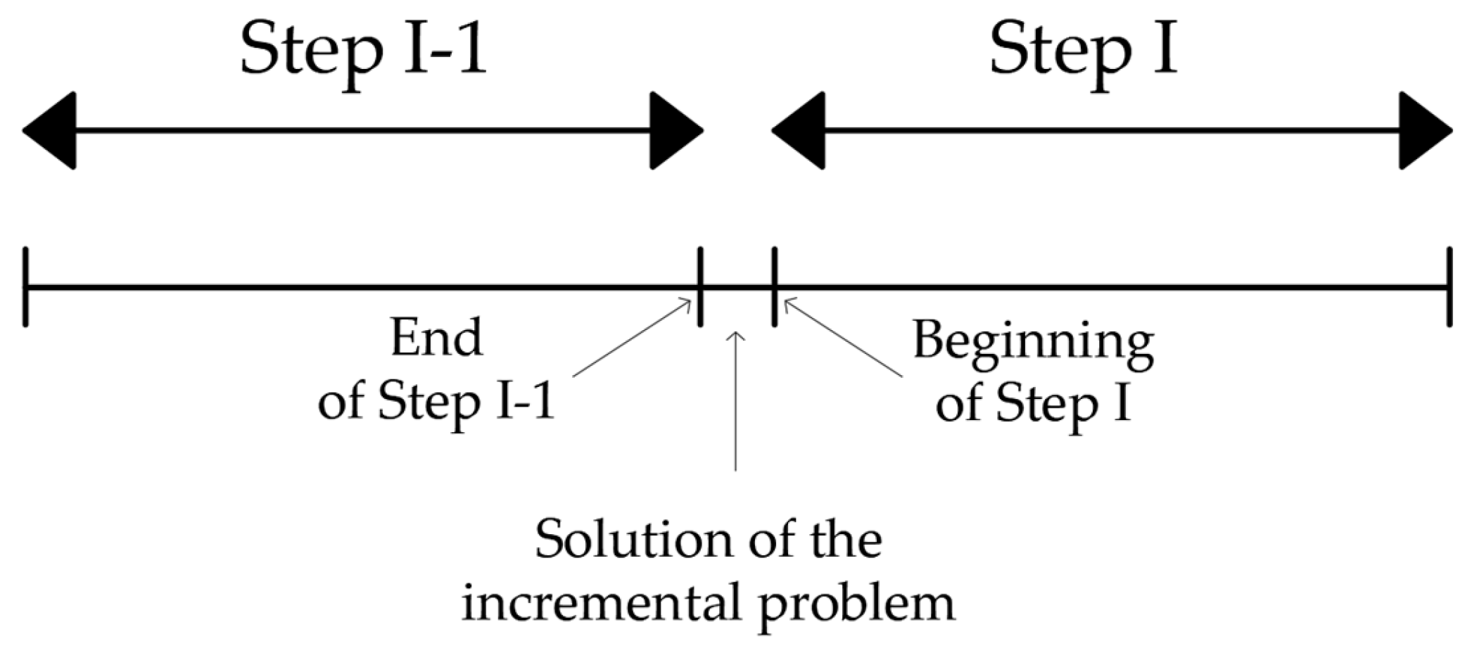
It is assumed that, at each step, a new $\mathsf{\varphi }$ mode becomes active or is deactivated. The case of new activation is described as the loading program sequence, organized in a stepwise manner, where each main step spans a prescribed interval of the load parameter. It unfolds through a sequence of intermediate increments that advance the state from the beginning of the step to a uniquely defined terminal configuration. This representation emphasizes that the overall loading evolution is constructed by completing, step by step, an internal chain of intermediate updates until the end condition of the current step is reached. According to Figure 1, the solution of the incremental problem presented in the next section is performed at the beginning of the generic Step I.

3.1. Active Set and Reduced System

At a generic step $\mathrm{I}$, a subset of modes is active, meaning $\widehat{\mathsf{\varphi }}=0$ for those modes. Variables associated with active modes are collected with a hat (^∧):

• $\widehat{\Delta \mathsf{\lambda }}$ and $\widehat{\mathsf{\varphi }}$ denote restriction of $\Delta \mathsf{\lambda }$ and $\mathsf{\varphi }$ to active indices;
• ${\widehat{\mathbf{A}}}_{\mathrm{I}}$ denotes the restriction of $\mathbf{A}$ to active modes at step $\mathrm{I}$.

At the onset of Step $\mathrm{I}$, $(\mathrm{I}-1)$ ${\mathsf{\varphi }}_{\mathrm{i}}$ modes are active and the corresponding LCP is formulated on this active set. Upon the completion of Step $\mathrm{I}$, deriving with respect to time Equation (1), the problem can be written equivalently as:

$$\{\begin{array}{cc}{\widehat{\dot{\mathsf{\varphi }}}}_{\mathrm{I}-1}& ={\widehat{\mathbf{A}}}_{\mathrm{I}-1}\hspace{0.17em}\Delta {\widehat{\dot{\mathsf{\lambda }}}}_{\mathrm{I}-1}+{\widehat{\mathbf{a}}}_{\mathrm{I}}\hspace{0.17em}\Delta {\widehat{\dot{\mathsf{\lambda }}}}_{\mathrm{I}}-\Delta \dot{\mathsf{\alpha }}\hspace{0.17em}{\widehat{\mathbf{b}}}_{\mathrm{I}-1}\\ {\widehat{\dot{\mathsf{\varphi }}}}_{\mathrm{I}}& ={\widehat{\mathbf{a}}}_{\mathrm{I}}^{\mathrm{t}}\hspace{0.17em}\Delta {\widehat{\dot{\mathsf{\lambda }}}}_{\mathrm{I}-1}+{\widehat{\mathrm{a}}}_{\mathrm{I}\mathrm{I}}\hspace{0.17em}\Delta {\widehat{\dot{\mathsf{\lambda }}}}_{\mathrm{I}}-\Delta \dot{\mathsf{\alpha }}\hspace{0.17em}{\widehat{\mathrm{b}}}_{\mathrm{I}}\end{array}$$

(15)

The active-mode matrix at step $I$ is:

$${\widehat{\mathbf{A}}}_{\mathrm{I}}=\left[\begin{array}{cc}{\widehat{\mathbf{A}}}_{\mathrm{I}-1}& {\widehat{\mathbf{a}}}_{\mathrm{I}}\\ {\widehat{\mathbf{a}}}_{\mathrm{I}}^{\mathrm{t}}& {\widehat{\mathrm{a}}}_{\mathrm{I}\mathrm{I}}\end{array}\right]$$

(16)

Assuming the problem is stable up to Step $\mathrm{I}-1$, stability at the end of Step $\mathrm{I}$ is examined through the properties of ${\widehat{\mathbf{A}}}_{\mathrm{I}}$. The inverse is expressed in the compatible block form:

$${\widehat{\mathbf{A}}}_{\mathrm{I}}^{-1}=\left[\begin{array}{cc}{\widehat{\mathbf{C}}}_{\mathrm{I}-1}& {\widehat{\mathbf{c}}}_{\mathrm{I}}\\ {\widehat{\mathbf{c}}}_{\mathrm{I}}^{\mathrm{t}}& {\widehat{\mathrm{c}}}_{\mathrm{I}\mathrm{I}}\end{array}\right]$$

(17)

with:

$${\widehat{\mathrm{c}}}_{\mathrm{I}\mathrm{I}}={\displaystyle \frac{1}{{\widehat{\mathrm{a}}}_{\mathrm{I}\mathrm{I}}-{\widehat{\mathbf{a}}}_{\mathrm{I}}^{\mathrm{t}}\hspace{0.17em}{\widehat{\mathbf{A}}}_{\mathrm{I}-1}^{-1}\hspace{0.17em}{\widehat{\mathbf{a}}}_{\mathrm{I}}}},{\widehat{\mathbf{c}}}_{\mathrm{I}}=-{\widehat{\mathbf{A}}}_{\mathrm{I}-1}^{-1}\hspace{0.17em}{\widehat{\mathbf{a}}}_{\mathrm{I}}\hspace{0.17em}{\widehat{\mathrm{c}}}_{\mathrm{I}\mathrm{I}}.$$

(18)

By the cofactor definition of the inverse:

$${\widehat{\mathrm{c}}}_{\mathrm{I}\mathrm{I}}={\displaystyle \frac{\mathrm{d}\mathrm{e}\mathrm{t}\left|{\widehat{\mathbf{A}}}_{\mathrm{I}-1}\right|}{\mathrm{d}\mathrm{e}\mathrm{t}\left|{\widehat{\mathbf{A}}}_{\mathrm{I}}\right|}}$$

(19)

hence:

$$\mathrm{d}\mathrm{e}\mathrm{t}\left|{\widehat{\mathbf{A}}}_{\mathrm{I}}\right|={\displaystyle \frac{\mathrm{d}\mathrm{e}\mathrm{t}\left|{\widehat{\mathbf{A}}}_{\mathrm{I}-1}\right|}{{\widehat{\mathrm{c}}}_{\mathrm{I}\mathrm{I}}}}$$

(20)

These relations provide the algebraic basis for stating the stability condition at the end of Step $\mathrm{I}$.

3.2. Stability and Uniqueness Condition

Given that $\mathrm{d}\mathrm{e}\mathrm{t}\mid {\widehat{\mathbf{A}}}_{\mathrm{I}-1}^{-1}\mid >0$, to ensure $\mathrm{d}\mathrm{e}\mathrm{t}\mid {\widehat{\mathbf{A}}}_{\mathrm{I}}\mid >0$, from Equation (20), it follows that:

$$\begin{array}{cccc}& {\displaystyle \frac{1}{{\widehat{\mathrm{a}}}_{\mathrm{I}\mathrm{I}}-{\widehat{\mathbf{a}}}_{\mathrm{I}}^{\mathrm{t}}\hspace{0.17em}{\widehat{\mathbf{A}}}_{\mathrm{I}-1}^{-1}\hspace{0.17em}{\widehat{\mathbf{a}}}_{\mathrm{I}}}}>0& & \end{array}$$

(21)

The condition to ensure that the problem remains semi-definite positive at the end of Step $I$ is:

$$\begin{array}{cccc}& {\widehat{\mathrm{a}}}_{\mathrm{i}\mathrm{i}}-{\widehat{\mathbf{a}}}_{\mathrm{i}}^{\mathrm{t}}\hspace{0.17em}{\widehat{\mathbf{A}}}_{\mathrm{i}-1}^{-1}\hspace{0.17em}{\widehat{\mathbf{a}}}_{\mathrm{i}}>0,\forall \hspace{0.17em}\mathrm{i}\le \mathrm{I}.& & \end{array}$$

(22)

Condition (22) extends the stepwise requirement to all intermediate augmentations up to index $\mathrm{I}$, ensuring that each successive active-mode extension preserves semi-definite positivity and, consequently, local uniqueness of the reduced incremental response within the active subspace.

To derive a further relation at the end of Step $\mathrm{I}-1$, with ${\widehat{\mathbf{A}}}_{\mathrm{I}-1}$ semi-definite positive, note that mode $\mathrm{I}$ is not yet active, i.e., $\Delta {\widehat{\dot{\mathsf{\lambda }}}}_{\mathrm{I}}=0$. Under this assumption, ${\dot{\mathsf{\varphi }}}_{\mathrm{I}}\le 0$. For:

$$\begin{array}{cccc}& {\widehat{\dot{\mathsf{\varphi }}}}_{\mathrm{I}-1}=0, \Delta {\widehat{\dot{\mathsf{\lambda }}}}_{\mathrm{I}}=0, \Delta \dot{\mathsf{\alpha }}\ge 0,& & \end{array}$$

(23)

the sign constraint $\Delta \dot{\mathsf{\alpha }}\ge 0$ fixes the direction of the increment, so that maintaining ${\dot{\mathsf{\varphi }}}_{\mathrm{I}}\le 0$ while $\Delta {\widehat{\dot{\mathsf{\lambda }}}}_{\mathrm{I}}=0$ enforces consistency of keeping mode $\mathrm{I}$ inactive at the end of Step $\mathrm{I}-1$.

By solving the first equation in (15) for $\Delta {\widehat{\dot{\mathsf{\lambda }}}}_{\mathrm{I}-1}$ and substituting it in the second equation of (15), the following inequality is obtained:

$${\dot{\mathsf{\varphi }}}_{\mathrm{I}}=\Delta \dot{\mathsf{\alpha }}({\widehat{\mathbf{a}}}_{\mathrm{I}}^{\mathrm{t}}\hspace{0.17em}{\widehat{\mathbf{A}}}_{\mathrm{I}-1}^{-1}{\widehat{\mathbf{b}}}_{\mathrm{I}-1}-{\widehat{\mathrm{b}}}_{\mathrm{I}})\le 0$$

(24)

Equation (24) represents the algebraic bridge, which links the end-of-step assumptions to the “activation-consistency” inequality, which results:

$${\widehat{\mathbf{a}}}_{\mathrm{I}}^{\mathrm{t}}\hspace{0.17em}{\widehat{\mathbf{A}}}_{\mathrm{I}-1}^{-1}{\widehat{\mathbf{b}}}_{\mathrm{I}-1}-{\widehat{\mathrm{b}}}_{\mathrm{I}}\le 0$$

(25)

Inequality (25) characterizes when mode $\mathrm{I}$ can remain inactive at the end of Step $\mathrm{I}-1$ under $\Delta \dot{\mathsf{\alpha }}\ge 0$. In Section 5, strict inequalities away from degenerate cases are used to relate the sign of $\Delta \dot{\mathsf{\alpha }}$ to the sign of the definiteness indicator in (21) and (22).

4. Handling Non-Holonomic Constraints

Certain modes may exhibit non-holonomic behavior, requiring:

$$\begin{array}{cccc}& \Delta {\widehat{\dot{\mathsf{\lambda }}}}_{\mathrm{i}}\ge 0, {\mathsf{\varphi }}_{\mathrm{i}}\hspace{0.17em}\Delta {\widehat{\dot{\mathsf{\lambda }}}}_{\mathrm{i}}=0& & \end{array}$$

(26)

A classical approach would reformulate an incremental LCP restricted to active non-holonomic variables and solve it with a complementary pivot method (e.g., Lemke [10]). While mathematically robust, this reduced-system solving algorithm may be more expensive than a single tableau pivot step, and it undermines the benefits of the fully matrix-based pivoting scheme.

In the present implementation, non-holonomic constraints are enforced by assigning a small positive rate $\Delta {\widehat{\dot{\mathsf{\lambda }}}}_{\mathrm{i}}$ to non-holonomic variables that are (i) basic and (ii) constrained to be non-decreasing. Theoretically, this corresponds to introducing negligible distortions into the system that do not significantly perturb the KKT equilibrium conditions. Specifically, at each step, a value of order ${10}^{-6}$ is given to $\Delta {\widehat{\dot{\mathsf{\lambda }}}}_{\mathrm{i}}$, and the accumulated inelastic variable is updated as:

$$(\Delta {\widehat{\mathsf{\lambda }}}_{\mathrm{I}}{)}_{\mathrm{i}}=(\Delta {\widehat{\mathsf{\lambda }}}_{\mathrm{I}-1}{)}_{\mathrm{i}}+(\Delta {\mathsf{\alpha }}_{\mathrm{I}}-\Delta {\mathsf{\alpha }}_{\mathrm{I}-1})\hspace{0.17em}\Delta {\widehat{\dot{\mathsf{\lambda }}}}_{\mathrm{i}}$$

(27)

This preserves the monotonicity of $\Delta {\mathsf{\lambda }}_{\mathrm{i}}$ while maintaining the tableau structure of the holonomic procedure.

5. Relation Between $∆\dot{\mathit{\alpha }}$ and the Definiteness of the Matrix $\widehat{\mathit{A}}$ in the Rate Problem

Consider the infinitesimal rate form of the active-mode problem under an infinitesimal load increment $\Delta \dot{\mathsf{\alpha }}\hspace{0.17em}\widehat{\mathbf{b}}$ expressed in Equation (15), it is assumed that ${\widehat{\mathbf{A}}}_{\mathrm{I}-1}$ is positive semi-definite.

By solving the first Equation (15) for $\Delta {\widehat{\dot{\mathsf{\lambda }}}}_{\mathrm{I}-1}$, it results:

$$\Delta {\widehat{\dot{\mathsf{\lambda }}}}_{\mathrm{I}-1}={\widehat{\mathbf{A}}}_{\mathrm{I}-1}^{-1}\left({\widehat{\dot{\mathsf{\varphi }}}}_{\mathrm{I}-1}-{\widehat{\mathbf{a}}}_{\mathrm{I}}\hspace{0.17em}\Delta {\widehat{\dot{\mathsf{\lambda }}}}_{\mathrm{I}}+\Delta \dot{\mathsf{\alpha }}\hspace{0.17em}{\widehat{\mathbf{b}}}_{\mathrm{I}-1}\right)$$

(28)

Equation (28) is substituted in the second Equation (15), which is solved for $\Delta \dot{\mathsf{\alpha }}$, resulting in:

$$\Delta \dot{\mathsf{\alpha }}={\displaystyle \frac{1}{{\widehat{\mathrm{b}}}_{\mathrm{I}}}}\left(-{\widehat{\dot{\mathsf{\varphi }}}}_{\mathrm{I}}+{\widehat{\mathbf{a}}}_{\mathrm{I}}^{\mathrm{t}}{\widehat{\mathbf{A}}}_{\mathrm{I}-1}^{-1}\left({\widehat{\dot{\mathsf{\varphi }}}}_{\mathrm{I}-1}-{\widehat{\mathbf{a}}}_{\mathrm{I}}\Delta \widehat{\dot{{\mathsf{\lambda }}_{\mathrm{I}}}}+\Delta \dot{\mathsf{\alpha }}{\widehat{\mathbf{b}}}_{\mathrm{I}-1}\right)+{\widehat{\mathrm{a}}}_{\mathrm{I}\mathrm{I}}{\Delta \widehat{\dot{\mathsf{\lambda }}}}_{\mathrm{I}}\right)$$

(29)

After some algebraic manipulation of (29), considering (23) and the activation condition ${\widehat{\dot{\mathsf{\varphi }}}}_{\mathrm{I}}=0$, the following equation is derived:

$$\Delta \dot{\mathsf{\alpha }}({\widehat{\mathrm{b}}}_{\mathrm{I}}-{\widehat{\mathbf{a}}}_{\mathrm{I}}^{\mathrm{t}}{\widehat{\mathbf{A}}}_{\mathrm{I}-1}^{-1}{\widehat{\mathbf{b}}}_{\mathrm{I}-1})=\Delta {\widehat{\dot{\mathsf{\lambda }}}}_{\mathrm{I}}({\widehat{\mathrm{a}}}_{\mathrm{I}\mathrm{I}}-{\widehat{\mathbf{a}}}_{\mathrm{I}}^{\mathrm{t}}{\widehat{\mathbf{A}}}_{\mathrm{I}-1}^{-1}{\widehat{\mathbf{a}}}_{\mathrm{I}}).$$

(30)

Recalling Equation (25), it may conclude that (under $\Delta {\widehat{\dot{\mathsf{\lambda }}}}_{\mathrm{I}}\ge 0$, with $\Delta {\mathsf{\lambda }}_{\mathrm{I}}=0$ at the end of Step $(\mathrm{I}-1$):

$$\Delta \dot{\mathsf{\alpha }}<0 \mathrm{if} {\widehat{\mathrm{a}}}_{\mathrm{I}\mathrm{I}}-{\widehat{\mathbf{a}}}_{\mathrm{I}}^{\mathrm{t}}{\widehat{\mathbf{A}}}_{\mathrm{I}-1}^{-1}{\widehat{\mathbf{a}}}_{\mathrm{I}}<0,$$

(31)

$$\Delta \dot{\mathsf{\alpha }}=0 \mathrm{if} {\widehat{\mathrm{a}}}_{\mathrm{I}\mathrm{I}}-{\widehat{\mathbf{a}}}_{\mathrm{I}}^{\mathrm{t}}{\widehat{\mathbf{A}}}_{\mathrm{I}-1}^{-1}{\widehat{\mathbf{a}}}_{\mathrm{I}}=0.$$

(32)

In other words, when the Hessian matrix ${\mathbf{A}}_{\mathrm{I}}$ becomes no more semi-definite positive at the end of step I, the procedure automatically proceeds with:

(1)

Activation of the last active mode ${\widehat{\dot{\mathsf{\varphi }}}}_{\mathrm{I}}=0$.

(2)

Decrease in the load factor $\Delta \dot{\mathsf{\alpha }}\le 0$.

It is important to emphasize that the solution procedure remains consistent regardless of the definiteness of the reduced Hessian matrix Ȃ. Specifically, the algorithm operates under the same logic whether Ȃ is positive semi-definite or indefinite. A key feature of the procedure is the requirement that a crack mode activated at step I-1 must remain active in the subsequent step I. This algorithmic constraint is fundamental, as it allows the procedure to distinguish the physical equilibrium path from a simple unloading state during the descending branch of the load factor (α).

6. Limit Load and Collapse Mechanism

Within the tableau procedure, a collapse mechanism (limit point) can be detected when the pivoting required to maintain feasibility produces a configuration where further progress in the controlling variable is impossible while preserving complementarity.

Let a tableau at step $\mathrm{I}$ contain a row $\mathrm{k}$ associated with the basic variable $\mathsf{\alpha }$ such that $\mathrm{T}(\mathrm{k},1)=\mathsf{\alpha }\ge 0$, and consider a candidate entering column $\mathrm{m}+1$ associated with an out-of-basis variable (

Table 3. Tableau at collapse.

		${\mathrm{x}}_1$	${\mathrm{x}}_2$	…	${\mathrm{x}}_{\mathrm{n}}$$= {\mathsf{\varphi }}_{\mathrm{k}}$	…	${\mathrm{x}}_{\mathrm{m}}=$$\Delta {\mathsf{\lambda }}_{\mathrm{k}}$	…	${\mathrm{x}}_{{\mathrm{n}}_{\mathrm{y}}+1}$
${\mathrm{y}}_1$	T(1,1)	T(1,2)	T(1,3)	…	T(1,n+1)	…	$\mathrm{T}(1,\mathrm{m}+1)\ge$0	…	T(1,ny+2)
$⋮$	…	…	…	…	…	…	…	…	…
${\mathrm{y}}_{\mathrm{k}}=$α	T(k,1)	T(k,2)	T(k,3)	…	T(k,n+1)	…	$\mathrm{T}(\mathrm{k},\mathrm{m}+1) = 0$	…	T(k,ny+2)
$⋮$	…	…	…	…	…	…	…	…	…
${\mathrm{y}}_{{\mathrm{n}}_{\mathrm{y}}}$	T(ny,1)	T(ny,2)	T(ny,3)	…	T(ny,n+1)	…	$\mathrm{T}({\mathrm{n}}_{\mathrm{y}},\mathrm{m}+1)\ge$0	…	T(ny,ny+2)

). If:

• $\mathrm{T}(\mathrm{k},\mathrm{m}+1)=0$, and
• all entries in column $\mathrm{m}+1$ satisfy $\mathrm{T}(\mathrm{i},\mathrm{m}+1)\ge 0$ for $1\le \mathrm{i}\le {\mathrm{n}}_{\mathrm{y}}$.
  Then, the procedure identifies a collapse mechanism and terminates the stage. The mechanism is given by the column vector $\mathrm{T}\left(:,\mathrm{m}+1\right)$ interpreted as a mode combination with $\Delta {\dot{\mathsf{\lambda }}}_{\mathrm{i}}=1$ along the corresponding direction.

7. Limit Load and Descending Branch (Δα < 0)

When the active-mode matrix loses positive definiteness at step $\mathrm{I}$, i.e., as described by Equation (33), the load factor decreases while internal variables continue to evolve. In tableau terms, this corresponds to the sign change in the sensitivity coefficient $\mathrm{T}(\mathsf{\alpha },\Delta {\mathsf{\lambda }}_{\mathrm{j}})<0$ associated with the most recently activated mode as described in Table 3.

To follow the descending branch in a controlled manner, the procedure enforces that the last activated mode remains active:

$${\mathsf{\varphi }}_{\mathrm{I}}=0, \Delta {\mathsf{\lambda }}_{\mathrm{I}}>0$$

(33)

So that the computation proceeds with physically consistent softening evolution. From this point onwards, multiple admissible solutions may exist, and the analysis must incorporate multiplicity checks as described in the following section.

8. Multiplicity of Solutions and Degenerate Solutions

8.1. Degeneracy and Multiplicity

Multiplicity of solutions in complementarity-based structural problems is associated with a degenerate tableau, i.e., configurations in which at least one basic variable is exactly zero (or numerically indistinguishable from zero) [9,10]. In cracking analyses, degeneracy commonly arises near symmetric configurations where two competing crack evolutions are equally admissible [23].

Consider a tableau ${\mathrm{T}}_0$ in which:

• Two complementary variables out of basis are ${\mathsf{\varphi }}_{\mathrm{j}}$ and $\Delta {\mathsf{\lambda }}_{\mathrm{j}}$;
• A basic variable ${\mathsf{\varphi }}_{\mathrm{k}}$ satisfies ${\mathsf{\varphi }}_{\mathrm{k}}=0$ (degeneracy).
  The central question is whether this degenerate tableau admits more than one admissible pivot path leading to distinct feasible bases and therefore distinct equilibrium solutions.

8.2. Unique Continuation

Let T₀ be the current tableau and consider the coefficient ${\mathrm{T}}_0({\mathsf{\varphi }}_{\mathrm{k}},\Delta {\mathsf{\lambda }}_{\mathrm{j}})$. If:

$${\mathrm{T}}_0({\mathsf{\varphi }}_{\mathrm{k}},\Delta {\mathsf{\lambda }}_{\mathrm{j}})<0$$

(34)

then $\Delta {\mathsf{\lambda }}_{\mathrm{j}}$ can enter the basis via a standard feasibility-preserving pivot and remove the degeneracy. In this case, the continuation is unique (the algorithm selects the only admissible pivot that restores strict feasibility).

The occurrence of different solutions from this stage would mean that, starting from Tableau N.1 (

Table 4. Tableau N.1: First solution (active ${\Delta \mathsf{\lambda }}_{\mathrm{i}}$).

		${\mathsf{\varphi }}_{\mathrm{i}}$	${\Delta \mathsf{\lambda }}_{\mathrm{j}}$	${\mathsf{\varphi }}_{\mathrm{j}}$	${\Delta \mathsf{\lambda }}_{\mathrm{k}}$	$\Delta {\mathsf{\lambda }}_{\mathrm{r}}$
${\Delta \mathsf{\lambda }}_{\mathrm{i}}$	…	…	…	…	…	…
α	…	…	…	…	…	…
${\mathsf{\varphi }}_{\mathrm{k}}$	0 *	…	T0$({\mathsf{\varphi }}_{\mathrm{k}},{\Delta \mathsf{\lambda }}_{\mathrm{j}}$) > 0		T0$({\mathsf{\varphi }}_{\mathrm{k}},{\Delta \mathsf{\lambda }}_{\mathrm{k}}$) < 0	…
…	…	…	…	…	…	…

* or a very small positive value.

), different admissible bases can be obtained, leading to different sets of Δλᵢ in the basis.

Multiplicity becomes possible when the degenerate row exhibits the sign pattern ${\mathrm{T}}_0({\mathsf{\varphi }}_{\mathrm{k}},\Delta {\mathsf{\lambda }}_{\mathrm{j}})>0$ and ${\mathrm{T}}_0({\mathsf{\varphi }}_{\mathrm{k}},\Delta {\mathsf{\lambda }}_{\mathrm{k}})<0$; in this case, a void transformation on ${\mathrm{T}}_0({\mathsf{\varphi }}_{\mathrm{k}},\Delta {\mathsf{\lambda }}_{\mathrm{k}})$ provides an alternative admissible tableau (Tableau N.2,

Table 5. Tableau N.2: Second solution (active Δλ_i and Δλ_k).

		${\mathsf{\varphi }}_{\mathrm{i}}$	${\Delta \mathsf{\lambda }}_{\mathrm{j}}$	${\mathsf{\varphi }}_{\mathrm{j}}$	${\mathsf{\varphi }}_{\mathrm{k}}$	$\Delta {\mathsf{\lambda }}_{\mathrm{r}}$
${\Delta \mathsf{\lambda }}_{\mathrm{i}}$	…	…	…	…	…	…
α	…	…	…	…	…	…
$\Delta {\mathsf{\lambda }}_{\mathrm{k}}$	0 ∗	…	${\displaystyle \frac{-{\mathrm{T}}_0({\mathsf{\varphi }}_{\mathrm{k}},{\Delta \mathsf{\lambda }}_{\mathrm{j}})}{{\mathrm{T}}_0({\mathsf{\varphi }}_{\mathrm{k}},{\Delta \mathsf{\lambda }}_{\mathrm{k}})}}>0$		${\displaystyle \frac{1}{{\mathrm{T}}_0({\mathsf{\varphi }}_{\mathrm{k}},{\Delta \mathsf{\lambda }}_{\mathrm{k}})}}<0$	…
…	…	…	…	…	…	…

∗ or a very small positive value.

).

8.3. Constructive Second Solution and Void Transformation

A practical multiplicity criterion at tableau ${\mathrm{T}}_0$ is:

• A basic mode is degenerate:

$${\mathrm{T}}_0({\mathsf{\varphi }}_{\mathrm{k}},1)={\mathsf{\varphi }}_{\mathrm{k}}=0$$

(35a)

b.

The complementary entry is negative:

$${\mathrm{T}}_0({\mathsf{\varphi }}_{\mathrm{k}},\Delta {\mathsf{\lambda }}_{\mathrm{k}})<0$$

(35b)

c.

A cross-entry is positive:

$${\mathrm{T}}_0({\mathsf{\varphi }}_{\mathrm{k}},\Delta {\mathsf{\lambda }}_{\mathrm{j}})>0$$

(35c)

When (35) holds, a void transformation (a pivot of arbitrarily small amplitude, used as a basis exchange) can be performed with the pivot element ${\mathrm{T}}_0({\mathsf{\varphi }}_{\mathrm{k}},\Delta {\mathsf{\lambda }}_{\mathrm{k}})$. This generates a second admissible tableau N.2 (Table 5) in which both $\Delta {\mathsf{\lambda }}_{\mathrm{k}}$ and $\Delta {\mathsf{\lambda }}_{\mathrm{j}}$ may become simultaneously active [21], leading to a distinct equilibrium branch (for example, a symmetric crack evolution instead of an antisymmetric one).

This mechanism provides a constructive, algorithmic way to generate a second admissible tableau and hence a second equilibrium continuation from the same degenerate configuration without introducing geometric imperfections.

9. Application: Two-Notched Direct Tension Benchmark

9.1. Benchmark Definition

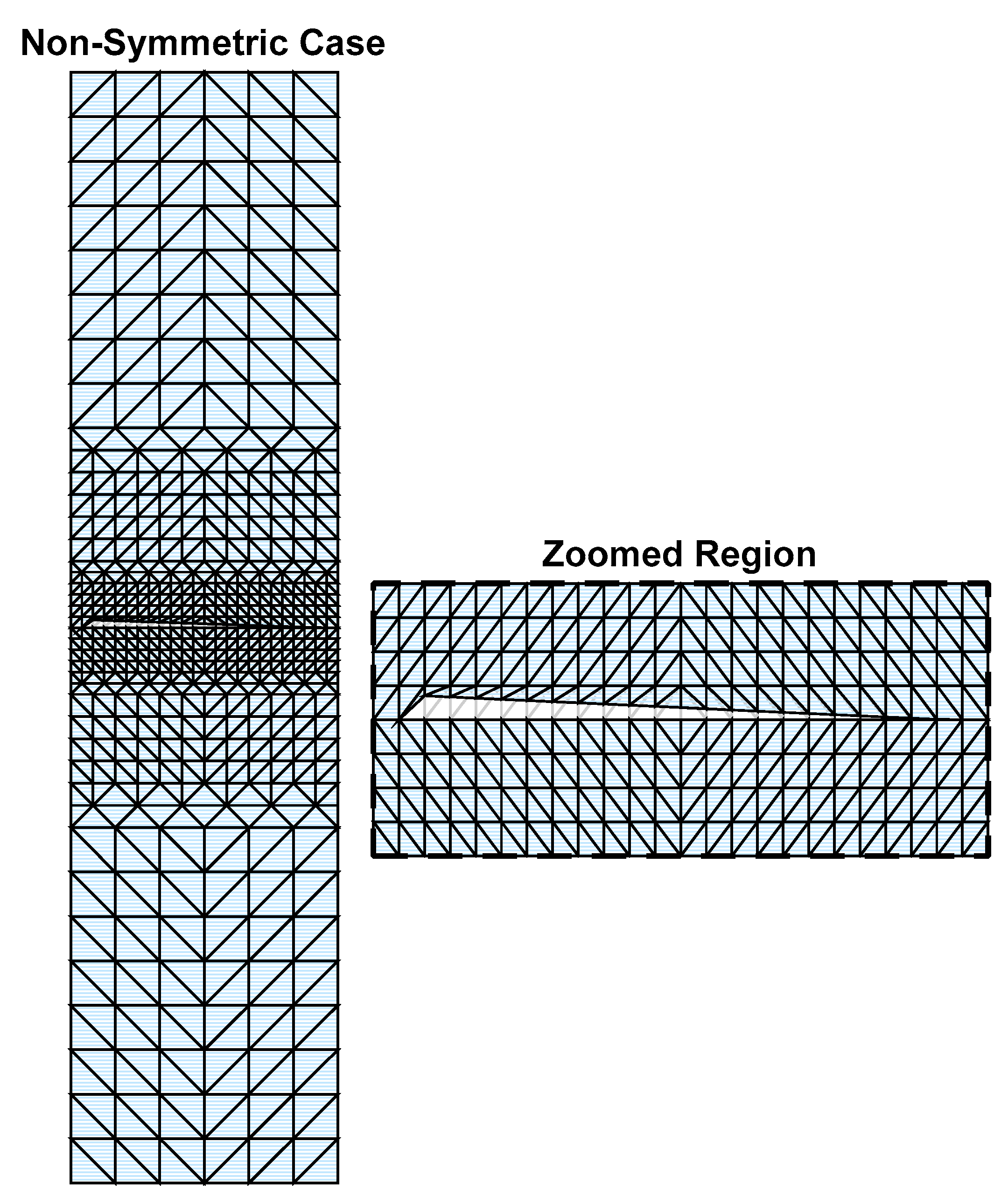
A classical two-notched 60 mm × 250 mm direct tension specimen, extensively documented in the scientific literature [11,19,20,23,26], is used to verify (i) the detection of the stability loss point and (ii) construction of competing symmetric/antisymmetric crack paths.

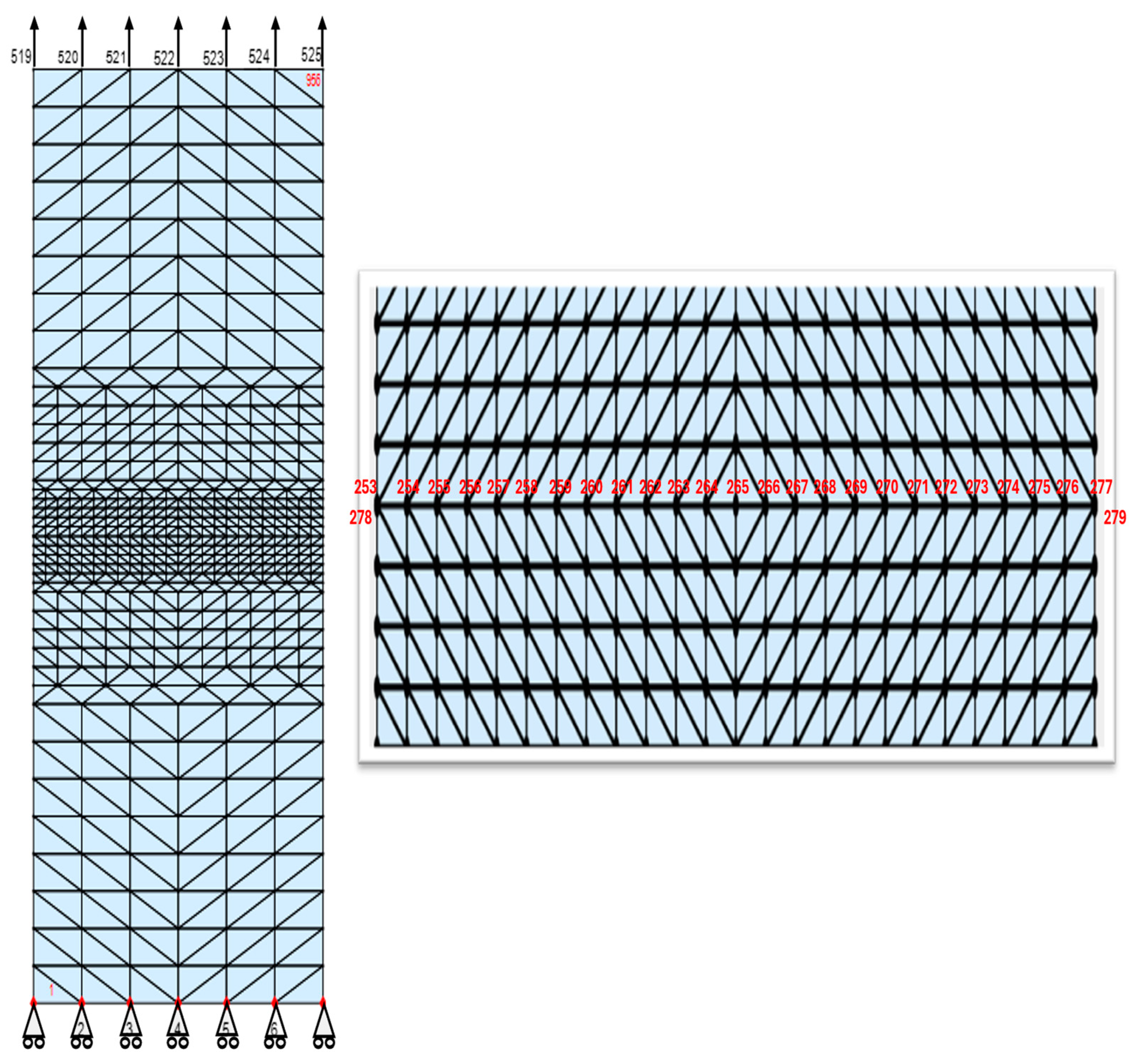
The two notches are introduced by duplicating the nodes of the mesh at the extremities of the central potential crack line, so that the upper and lower halves are kinematically disconnected at the notch locations (Figure 2). For instance, nodes 251–252 connect to lower elements, and duplicated nodes 526–527 (same coordinates) connect to upper elements. This standard “double-node” treatment reproduces the notch effect without modifying the crack-line topology, and it is consistent with the discrete crack-line representation adopted in the complementarity formulation [19].

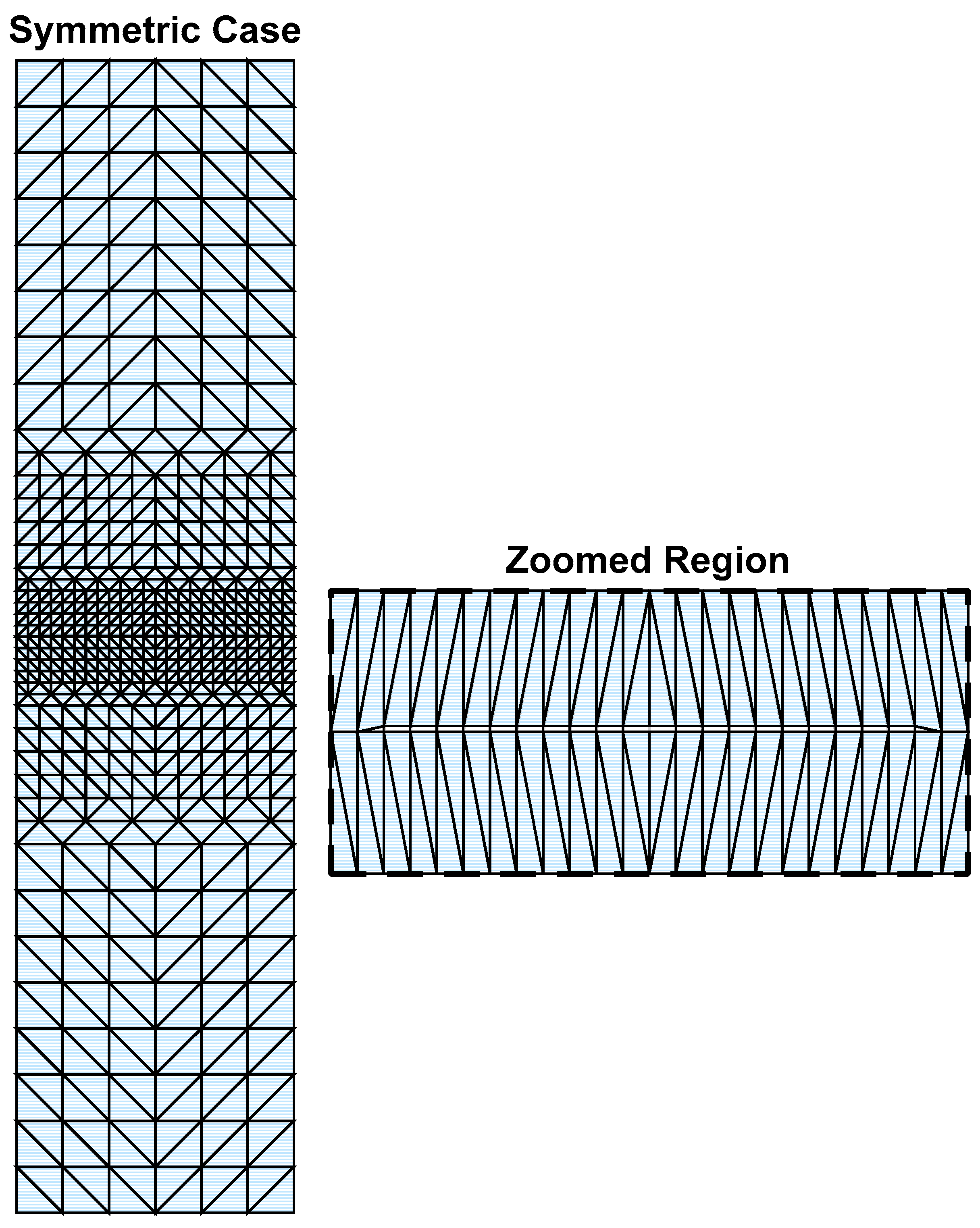
The specimen is discretized by a two-dimensional finite element mesh composed of nodes and three-node triangular plane stress/strain elements, with a constant thickness. Crack propagation is represented through a structured set of potential crack lines, giving potential cracking nodes (summed over all crack lines). The nonlinear response is formulated in a complementarity setting, with ${\mathrm{n}}_{\mathrm{y}}$ unknowns arranged in pairs $({\mathsf{\varphi }}_{\mathrm{i}},\Delta {\mathsf{\lambda }}_{\mathrm{i}})$, where ${\mathsf{\varphi }}_{\mathrm{i}}$ denotes the crack (gap/opening) mode variable and $\Delta {\mathsf{\lambda }}_{\mathrm{i}}$ its associated conjugate multiplier/normal force increment along each potential crack segment.

Summary of the three-node plane stress/strain triangular elements mesh features of the model are given in

Table 6. Mesh features of the model.

Nodes	Elements	Potential Crack Lines	Potential Cracking Nodes	Total Complementarity Unknowns (Pairs ${\mathit{\varphi }}_{\mathit{i}},\mathsf{\Delta }{\mathit{\lambda }}_{\mathit{i}}$)	Thickness
529	956	47	535	${\mathrm{n}}_{\mathrm{y}}$ = 1070	${\mathrm{t}}_{\mathrm{h}}=50$ mm

.

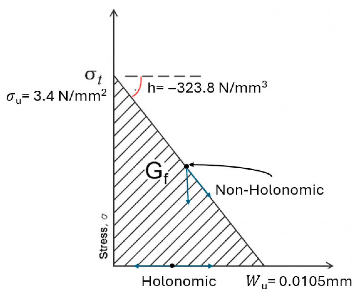
The constitutive behavior along potential crack interfaces follows the Hillerborg cohesive softening law [11,12], expressed in terms of normal traction (or normal force) vs. crack opening (Figure 3). The bulk material is defined by E = 37,000 N/mm² and $\nu =0.2$, while the softening branch is governed by the tensile strength σ_t = 3.4 N/mm² and the softening slope h = −323.8 N/mm² [19]. The ultimate opening W_u is obtained from:

$$\begin{array}{cccc}& {\mathsf{\sigma }}_{\mathrm{u}}={-\mathrm{W}}_{\mathrm{u}} \ast \mathrm{h}& & \end{array}\begin{array}{cccc}& {\mathrm{W}}_{\mathrm{u}}=-{\displaystyle \frac{{\mathsf{\sigma }}_{\mathrm{u}}}{\mathrm{h}}}=-{\displaystyle \frac{3.4}{323.8}}=0.0105 \mathrm{m}\mathrm{m}& & \end{array}$$

(36)

Along the central crack line, accounting for the two modes used to describe initiation/softening and the zero-stress opening/closing phase, the number of unknowns is 42.

9.2. Uncontrolled Multiplicity: Emergence of Antisymmetric Path

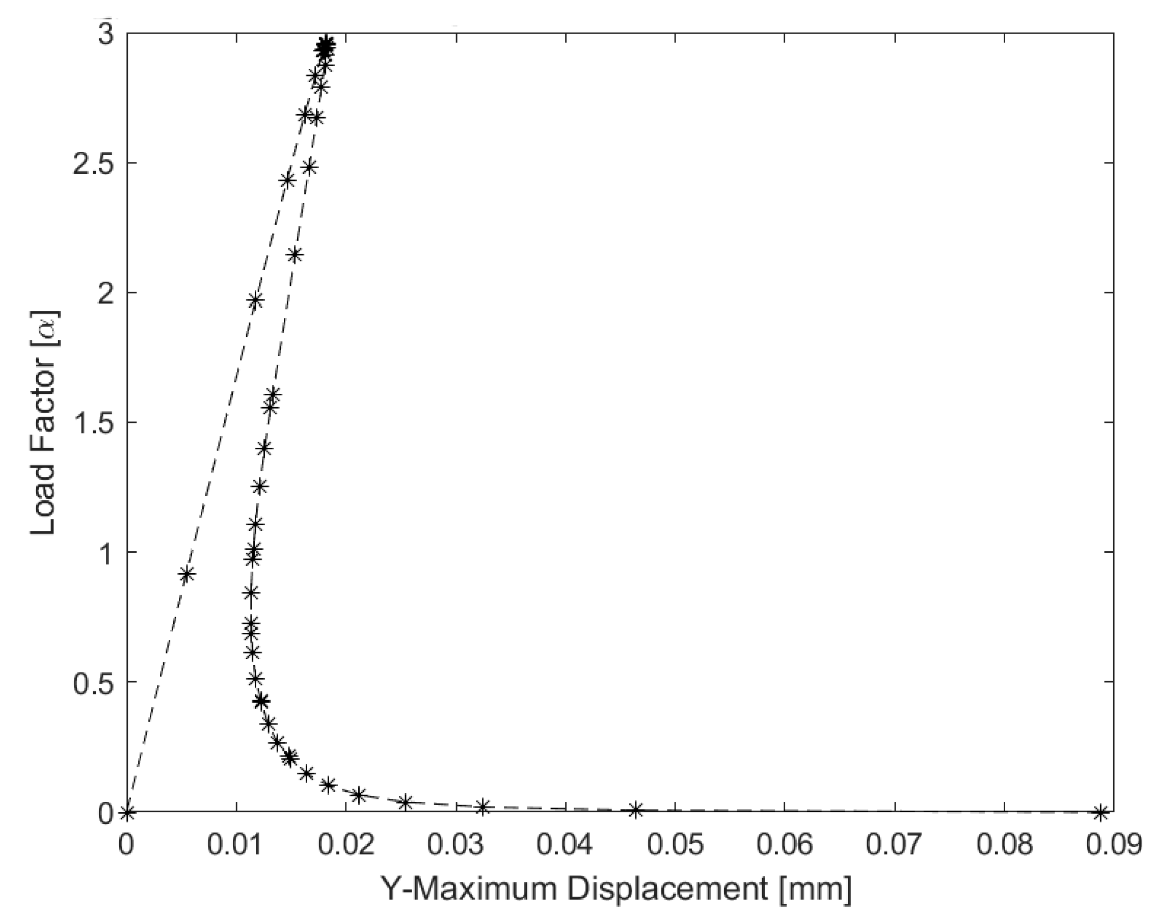
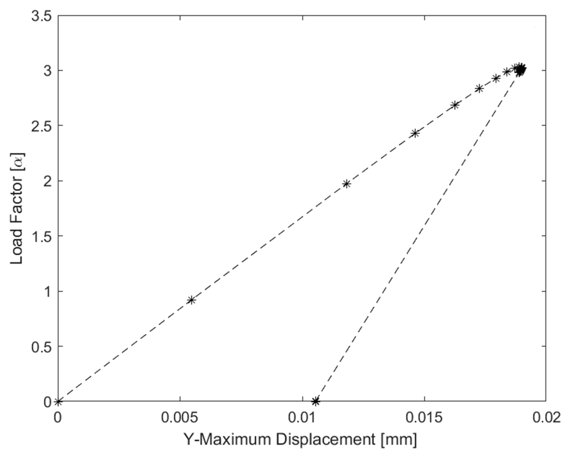
The computed history of $\mathsf{\alpha }$ increases from 0 to a maximum near $\mathsf{\alpha }\approx 2.96$ and then decreases to approximately zero along the softening branch. The full run takes 71 steps; the first elastic limit step ends at $\mathsf{\alpha }=0.9192$ (Figure 4).

From step 1 to 11, the path is stable. Softening modes activate alternately at symmetric locations, progressively advancing the crack from both notches. The activated nodes include (left/right pairs) 253/273, 254/272, 255/271, 256/270, 257/269, and 258.

During these initial elastic and stable-softening phases, the uniqueness of the solution is guaranteed by the positive definiteness of the reduced Hessian $\widehat{\mathbf{A}}$, which is evidenced by the sensitivity coefficients (T) in the tableau remaining consistently negative, forcing a unique pivot sequence and a monotonic increase in the load factor α.

At step 11, the coefficient

$$\mathrm{T}(\mathsf{\alpha },\Delta {\mathsf{\lambda }}_{\mathrm{j}})={\displaystyle \frac{\partial \mathsf{\alpha }}{\partial \Delta {\mathsf{\lambda }}_{\mathrm{j}}}}<0$$

(37)

indicates that $\widehat{\mathbf{A}}$ is no longer positive semi-definite, and multiplicity becomes possible.

From step 12 to 20, the post-critical switching takes place. For increasing $\alpha$, once the Hessian matrix is no longer semi-definite positive, the response exhibits activation/unloading events that can be detailed as follows: node 273 unloads (Step 12), node 268 activates (Step 13), node 272 unloads (Step 14), node 259 activates (Step 15), node 270 unloads (Step 16), node 271 unloads (Step 17), node 269 unloads (Step 18), node 260 activates (Step 19), and node 268 unloads (Step 20). The capability to deal with this non-holonomic behavior is crucial.

The structure is symmetric and, in principle, softening modes at nodes (e.g., 253 and 273) should activate contemporaneously. Owing to numerical imprecision, the softening mode is activated first at node 253, while the corresponding mode at node 273 remains positive, although possibly very small. At the second step, the increment of $\mathsf{\alpha }$ is very small, with $\mathrm{T}(\mathsf{\alpha },\Delta {\mathsf{\lambda }}_{\mathrm{j}})>0$ where j denotes the last activated mode, and perfect symmetry is re-established (both ${\mathsf{\varphi }}_{\mathrm{i}}$ modes are out of the basis). As a consequence, the solution at odd steps (1, 3, 5, 7, 9, 11) is degenerate, whereas at even steps (2, 4, 6, 8, 10) it is not degenerate. In odd steps ($\mathrm{T}({\mathsf{\varphi }}_{\mathrm{k}},\Delta {\mathsf{\lambda }}_{\mathrm{j}})<0$) the small positive value assigned to ${\mathsf{\varphi }}_{\mathrm{k}}$, which induces a slight asymmetry, is nullified in the subsequent even step and symmetry is restored.

Here, $\mathrm{T}(\mathsf{\alpha },\Delta {\mathsf{\lambda }}_{\mathrm{j}})$ denotes the coefficient of matrix $\mathrm{T}$ in the row associated with the variable $\mathsf{\alpha }$ and the column associated with $\Delta {\mathsf{\lambda }}_{\mathrm{j}}$; if it is positive, the load factor $\mathsf{\alpha }$ increases when $\Delta {\mathsf{\lambda }}_{\mathrm{j}}$ enters the basis.

The limit load is defined as the maximum load attained while $\widehat{\mathbf{A}}$ remains positive semi-definite. At Step $\mathrm{N}=11$ (odd) $\mathsf{\alpha }=2.9288$. At this stage, 6 crack nodes are active on the left, and 5 nodes are active on the right. Since $\mathrm{T}(\mathsf{\alpha },\Delta {\mathsf{\lambda }}_{\mathrm{j}})<0$, matrix $\widehat{\mathrm{A}}$ is no longer positive semi-definite. Moreover, $\mathrm{T}({\mathsf{\varphi }}_{\mathrm{k}},\Delta {\mathsf{\lambda }}_{\mathrm{j}})>0$, therefore the symmetric behaviour terminates, and the antisymmetric solution branch is initiated.

Beyond this point, numerical perturbations may trigger an antisymmetric evolution: crack opening continues on one side while previously activated nodes unload on the opposite side. The load factor decreases monotonically, while the constitutive law transitions from softening to the zero-stress opening/closing mode.

The procedure terminates at Step 71 with $\mathsf{\alpha }=2.029\times {10}^{-12}$. At this stage, all tensile points on the left satisfy ${\mathsf{\sigma }}_{\mathrm{t}}=0$ up to node 271. Node 272 remains on the softening branch, and the last active point in the elastic regime is located immediately ahead of it. The resulting configuration corresponds to a collapse mechanism (Figure 5) characterized by a clockwise rotation of the section, with rotation taking place about the extreme node on the right, which acts as the kinematic pivot of the final mechanism.

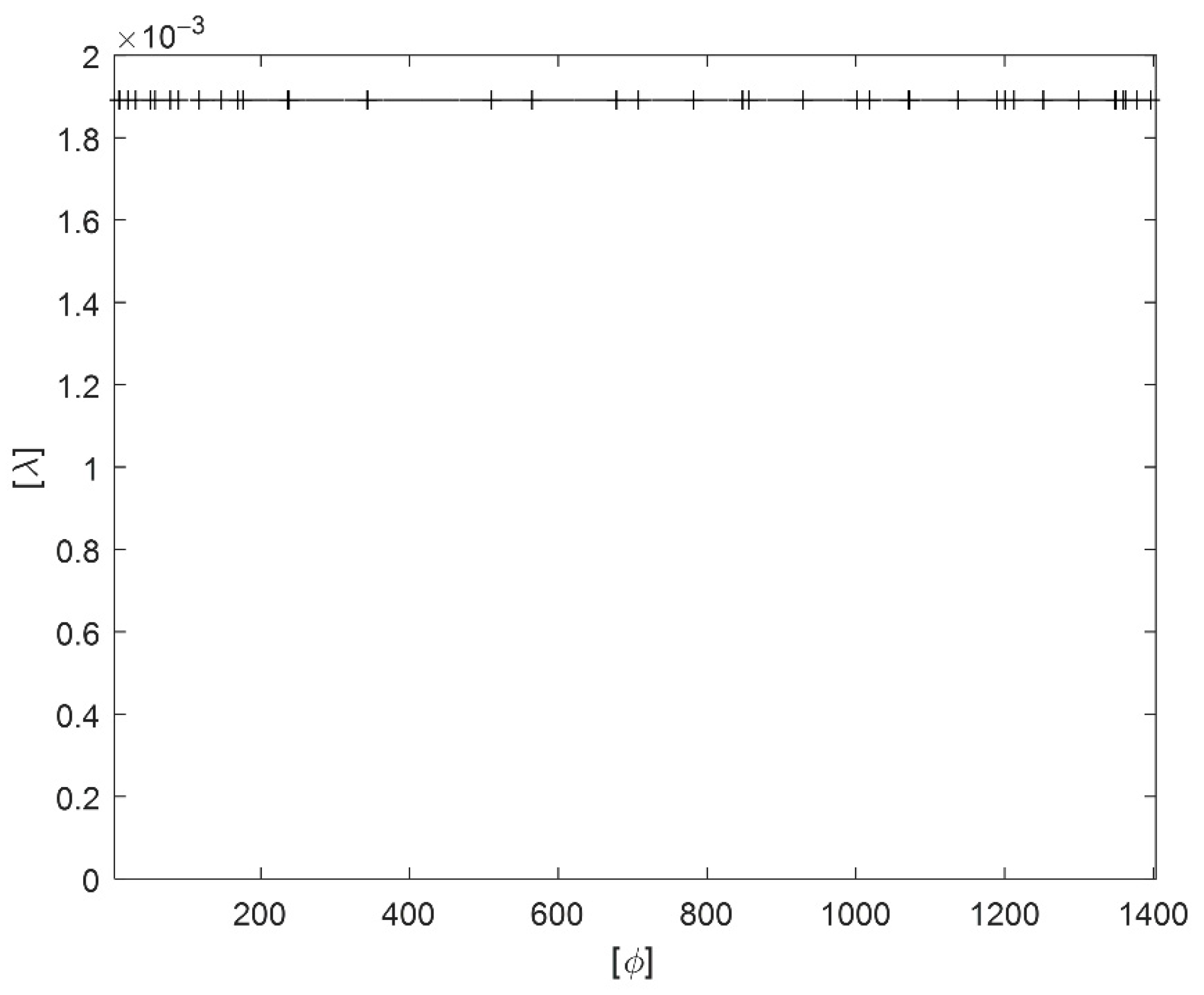
The non-holonomic behavior in terms of plastic variables is described in Figure 6, where at $\Delta \mathsf{\lambda }=1.8\times {10}^{-3}\hspace{0.17em}\mathrm{mm}$ the mode unloads: the multiplier no longer increases, $\Delta \mathsf{\lambda }$ remains constant, and the complementary variable switches so that $\mathsf{\varphi }$ changes from 0 to positive. This constant—$\Delta \mathsf{\lambda }$ switch indicates non-holonomic (history-dependent) behaviour.

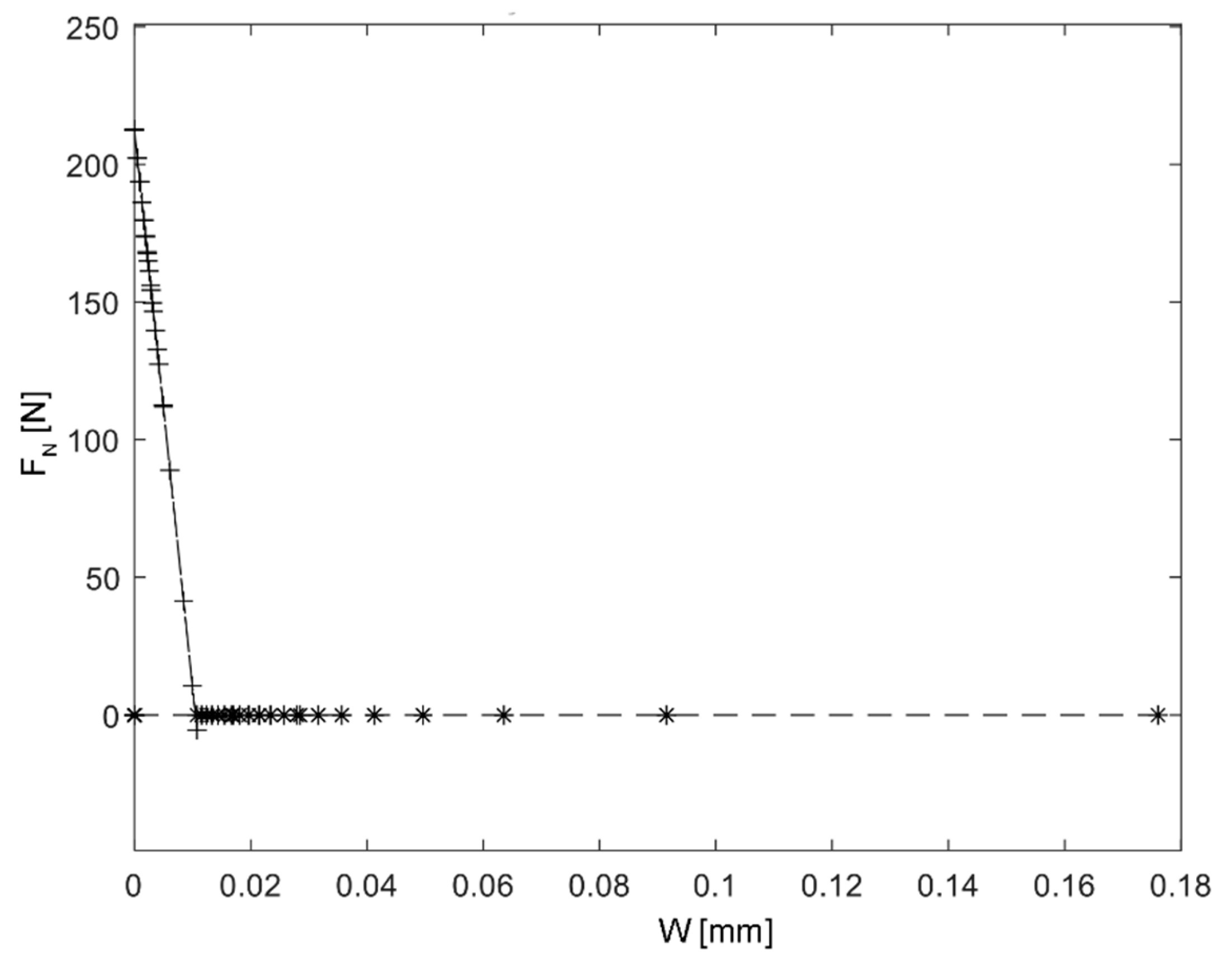
Figure 7 depicts the inelastic response of node 253 in the $({\mathrm{F}}_{\mathrm{N}},\mathrm{W})$ plane (normal force vs. crack opening). Two regimes are observed. In the first, ${\mathrm{F}}_{\mathrm{N}}>0$, the point evolves along the softening branch (mode 555): the crack opening increases while the normal force decreases according to the softening law, and the evolution is non-holonomic. In the second regime, ${\mathrm{F}}_{\mathrm{N}}=0$, the solution lies on the zero-traction branch (mode 556): the constraint ${\mathrm{F}}_{\mathrm{N}}=0$ is enforced and the crack opening may either increase (further opening) or decrease (partial closing), i.e., the response in this regime is holonomic.

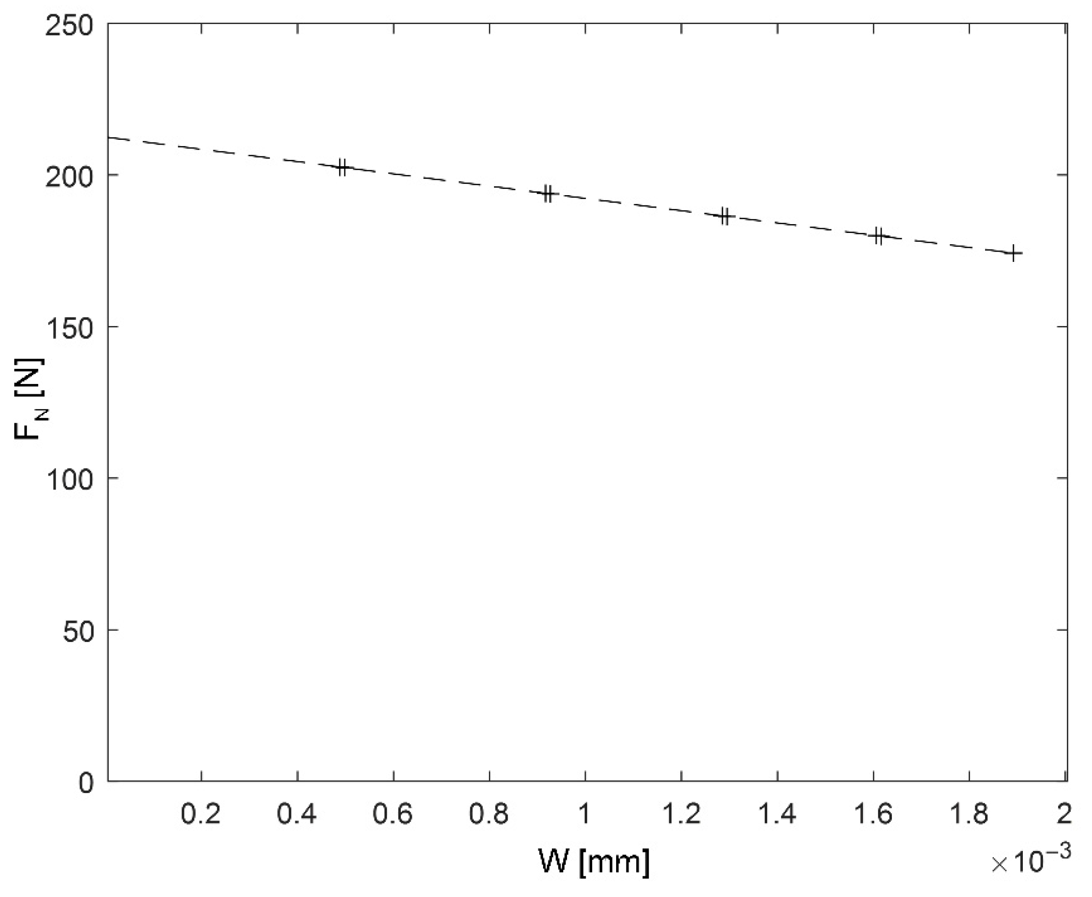
For the symmetric node along the main critical crack path, the behavior in terms of normal force and crack opening figures the initial softening response of mode 515, followed by unloading in the elastic range of the normal stress normal to the crack line, caused by the non-symmetric behavior of the specimen (Figure 8).

9.3. Controlled Multiplicity: Construction of a Symmetric Solution

When multiplicity conditions are detected at the critical step (Step 11), the algorithm applies the degeneracy criterion and performs a void pivot to generate the alternative tableau that enforces symmetric activation, which produces a different load displacement curve (Figure 9).

At step 11 ($\mathsf{\alpha }=2.9288$) the critical quantities are:

• $\mathrm{T}(\mathsf{\alpha },\Delta {\mathsf{\lambda }}_{\mathrm{j}})=-322.64$, with $\mathrm{j}=545$ corresponding to node 268.

Hence, the matrix $\widehat{\mathbf{A}}$ is no longer positive semi-definite and multiple solutions are possible. The multiplicity conditions are verified as follows:

• $\mathrm{T}({\mathsf{\varphi }}_{\mathrm{k}},1)=0$ (degenerate solution);
• $\mathrm{T}({\mathsf{\varphi }}_{\mathrm{k}},\Delta {\mathsf{\lambda }}_{\mathrm{j}})=8.6116\times {10}^5$, with $\mathrm{k}=525$ corresponding to node 268;
• $\mathrm{T}({\mathsf{\varphi }}_{\mathrm{k}},\Delta {\mathsf{\lambda }}_{\mathrm{k}})=-8.6116\times {10}^5$.

Node 268 lies on the right side of the central crack line and is symmetric to node 258. The procedure activates (i.e., brings into the basis) the mode $\Delta {\mathsf{\lambda }}_{\mathrm{k}}$ by a void pivot transformation. The resulting tableau has a positive coefficient $\mathrm{T}(\Delta {\mathsf{\lambda }}_{\mathrm{k}},\Delta {\mathsf{\lambda }}_{\mathrm{j}})$, so that letting $\Delta {\mathsf{\lambda }}_{\mathrm{j}}$ enter the basis increases $\Delta {\mathsf{\lambda }}_{\mathrm{k}}$, leading to a symmetric response (Figure 10).

Before the void pivot transformation, $\mathrm{T}(\mathsf{\alpha },\Delta {\mathsf{\lambda }}_{545})<0$. After the void pivot transformation, the same coefficient becomes greater than zero, meaning that increasing $\Delta {\mathsf{\lambda }}_{545}$ increases the load factor $\mathsf{\alpha }$.

The final mechanism is a symmetric opening mode dominated by tensile separation along the midline, with no marked lateral bias, consistent with the mirrored crack evolution on the two sides.

9.4. Numerical Remarks

(i).

The solution of the problem considered (529 nodes, 956 elements, 47 potential crack lines, 1070 unknowns ${\mathsf{\lambda }}_{\mathrm{i}}$) on a PC equipped with an Intel i7-13700 processor requires approximately 8 s. The computational benefit of parallel computing for the pivot-transformation computations was observed.

(ii).

In the present case, the nonlinear material behavior is described by a piecewise-linear model. The material law is formulated in terms of the stress vector acting on a potential linear cracking line, and the yield conditions are represented by two Coulomb straight lines and one cut-off straight line in the $({\mathsf{\sigma }}_{\mathrm{n}},\mathsf{\tau })$ plane (normal and shear stresses).

(iii).

For the stable part of the loading path, a comparison with the standard Newton method, adopted in nonlinear structural codes for problems with nonlinear material behavior, can be made. The Newton method is applied by subdividing the load factor into a predefined number of equal increments; within each increment, the response is nonlinear and Equation (5) is not considered, i.e., holonomic behavior is assumed. In the Mathematical Programming (MP) approach, the load increment is adjusted by the algorithm so that, within each step, the response is linear. The MP solution is exact with respect to the adopted piecewise-linear model, whereas the Newton solution is incremental and therefore approximate; increasing the number of Newton increments reduces this difference and leads to practically same results [27]. For the unstable part of the loading path, this paper notes that there is no unique continuation approach within a Newton framework, whereas the MP scheme described in this work provides a defined procedure.

(iv).

To validate the proposed tableau-based stability test, a direct verification was performed at the critical step where the sensitivity coefficient changed sign. The active-mode Hessian matrix $\widehat{\mathbf{A}}$ was extracted and its definiteness was checked through a standard LDL factorization. The results confirm that the first occurrence of a non-positive diagonal entry in the factorized matrix D, indicating a loss of positive definiteness, perfectly coincides with the output provided by the tableau pivot sequence. This numerical cross-check confirms that the proposed method effectively monitors structural stability.

10. Conclusions

This paper presented a tableau-based PLCP procedure for finite element cracking analyses with softening, together with a stability test and a constructive method for solution multiplicity.

1.

A stability/uniqueness criterion was formulated by monitoring the positive definiteness of the active-mode matrix $\widehat{\mathbf{A}}$ through a complement condition that can be evaluated incrementally during tableau progression.

2.

A direct relationship between the sign of the incremental load factor $\Delta \dot{\alpha }$ and the definiteness of $\widehat{\mathbf{A}}$ was established, providing an intrinsic indicator for transition to descending response without eigenvalue computations.

3.

A practical multiplicity mechanism was introduced: when a degenerate tableau satisfies a sign-structured criterion on key entries, a void pivot generates an alternative admissible tableau and hence a distinct equilibrium branch.

4.

The benchmark two-notched tension test demonstrated the ability of the method to construct symmetric and anti-symmetric crack evolutions from the same structural model, and to handle non-holonomic behavior consistently.

These results strengthen the role of complementarity programming in nonlinear structural analysis by providing computationally efficient tools for stability assessment and systematic exploration of competing failure mechanisms.

While the current study focuses on classic benchmarks to validate the stability test, further investigations involving more complex mixed-mode geometries and extensive sensitivity analyses are already underway and will be presented in future works. Future work will also focus on refining the tolerance definitions for identifying zeros within the procedure, particularly when optional unloading steps are permitted.

References

1. de Borst, R.; Crisfield, M.A.; Remmers, J.J.C.; Verhoosel, C.V. Nonlinear Finite Element Analysis of Solids and Structures, 2nd ed.; John Wiley & Sons, Ltd.: Hoboken, NJ, USA, 2012. [Google Scholar]
2. Karihaloo, B.L.; Huang, X. Tensile Response of Quasi-Brittle Materials. Pure Appl. Geophys. 1991, 137, 461–487. [Google Scholar] [CrossRef]
3. Bazant, Z.P.; Cedolin, L.; Hutchinson, J.W. Stability of Structures: Elastic, Inelastic, Fracture, and Damage Theories. J. Appl. Mech. 1993, 60, 567–568. [Google Scholar] [CrossRef]
4. Gastebled, O.J.; May, I.M. Bifurcation in the Numerical Simulation of Softening Mechanisms. Comput. Struct. 2000, 78, 745–755. [Google Scholar] [CrossRef]
5. Dawud, S.; Jawad, S. Stability Analysis of a Competitive Ecological System in a Polluted Environment. Commun. Math. Biol. Neurosci. 2022, 2022, 70. [Google Scholar] [CrossRef]
6. Bolzon, G.; Maier, G. Holonomic and Nonholonomic Simulations of Quasi-Brittle Fracture: A Comparative Study of Mathematical Programming Approaches. In Proceedings of the Fracture Mechanics of Concrete Structures, Proceedings FRAMCOS-2; Folker, H.W., Ed.; AEDIFICATIO Publishers: Freiburg, Germany, 1995; pp. 1529–1538. [Google Scholar]
7. Maier, G. A Quadratic Programming Approach for Certain Classes of Non Linear Structural Problems. Meccanica 1968, 3, 121–130. [Google Scholar] [CrossRef]
8. Best, M.J.; Ritter, K. Linear Programming: Active Set Analysis and Computer Programs; Prentice-Hall: Upper Saddle River, NJ, USA, 1985; ISBN 0135369967. [Google Scholar]
9. Maier, G. A Matrix Structural Theory of Piecewise Linear Elastoplasticity with Interacting Yield Planes. Meccanica 1970, 5, 54–66. [Google Scholar] [CrossRef]
10. Lemke, C.E. On Complementary Pivot Theory. In Mathematics of the Decision Sciences: Part 1; Amer Mathematical Society: Providence, RI, USA, 1968; Volume 11, pp. 95–114. [Google Scholar]
11. Hillerborg, A.; Modeer, M.; Petersson, P.E. Analysis of Crack Formation and Crack Growth in Concrete by Means of Fracture Mechanics and Finite Elements. Cem. Concr. Res. 1976, 6, 733–781. [Google Scholar] [CrossRef]
12. Hillerborg, A. Mixed Mode Fracture in Concrete. In Proceedings of the 7th International Conference On Fracture (ICF7), Houston, TX, USA, 20–24 March 1989; pp. 2259–2268. [Google Scholar] [CrossRef]
13. De Donato, O.; Paterlini, F. Historical Elastic-Plastic Analysis by PLCP and RBLP. In Proceedings of the Engineering Plasticity by Mathematical Programming, Proceedings of the NATO Advanced Study Institute; Cohn, M.Z., Maier, G., Eds.; Pergamon Press Inc.: New York, NY, USA, 1979. [Google Scholar]
14. Colonnetti, G. Elastic Equilibrium in the Presence of Permanent Set. Q. Appl. Math. 1950, 7, 353–362. [Google Scholar] [CrossRef][Green Version]
15. De Donato, O.; Maier, G. Historical Deformation Analysis of Elastoplastic Structures as a Parametric Linear Complementarity Problem. Meccanica 1976, 11, 166–171. [Google Scholar] [CrossRef]
16. Hodge, P.G., Jr. Automatic Piecewise Linearization in Ideal Plasticity. Comput. Methods Appl. Mech. Eng. 1977, 10, 249–272. [Google Scholar] [CrossRef]
17. Cottle, R.W.; Dantzig, G.B. Complementary Pivot Theory of Mathematical Programming. Linear Algebra Appl. 1968, 1, 103–125. [Google Scholar] [CrossRef]
18. Cottle, R.W. Monotone Solutions of the Parametric Linear Complementarity Problem. Math. Program. 1972, 3, 210–224. [Google Scholar] [CrossRef]
19. Scamardo, M.; Franchi, A.; Crespi, P. A Non-Standard Numerical Method for Finite Element Modelling of Tensile Cracks in Quasi-Brittle Material. Comput. Struct. 2022, 258, 106664. [Google Scholar] [CrossRef]
20. Bolzon, G.; Maier, G.; Tin-Loi, F. On Multiplicity of Solutions in Quasi-Brittle Fracture Computations. Comput. Mech. 1997, 19, 511–516. [Google Scholar] [CrossRef]
21. Franchi, A.; Genna, F.; Corradi, L. On the Determination of Bifurcation and Limit Points. J. Eng. Mech. 1998, 124, 866–874. [Google Scholar] [CrossRef]
22. Bassi, A.; Aravas, N.; Genna, F. A Linear Complementarity Formulation of Rate-Independent Finite-Strain Elastoplasticity. Part II: Calculation of Bifurcation and Limit Points. Eur. J. Mech. A/Solids 2012, 35, 128–137. [Google Scholar] [CrossRef]
23. Tin-Loi, F.; Tseng, P. Efficient Computation of Multiple Solutions in Quasibrittle Fracture Analysis. Comput. Methods Appl. Mech. Eng. 2003, 192, 1377–1388. [Google Scholar] [CrossRef]
24. Franchi, A.; Genna, F. A Numerical Scheme for Integrating the Rate Plasticity Equations with an “a Priori” Error Control. Comput. Methods Appl. Mech. Eng. 1987, 60, 317–342. [Google Scholar] [CrossRef]
25. Cottle, R.W.; Veinott, A.F. Polyhedral Sets Having a Least Element. Math. Program. 1972, 3, 238–249. [Google Scholar] [CrossRef]
26. Rots, J.G.; de Borst, R. Analysis of Concrete Fracture in “Direct” Tension. Int. J. Solids Struct. 1989, 25, 1381–1394. [Google Scholar] [CrossRef]
27. Rodigari, D.; Franchi, A.; Genna, F.; Crespi, P.; De Col, R. A Linear Complementarity Approach to the Time Integration of Dynamic Elastic–Plastic Structural Problems. Meccanica 2019, 54, 1597–1609. [Google Scholar] [CrossRef]
Figure 1. Sequence of loading steps.
Mathematics 14 01206 g001
Figure 2. Two-notched direct tension test model. The nodes highlighted in red are the ones involved in the progressively advancing crack.
Mathematics 14 01206 g002
Figure 3. The elastic-softening constitutive diagram in terms of normal force vs. crack opening.
Mathematics 14 01206 g003
Figure 4. Load ( α ) vs. vertical displacement of node 522 in the case of non-symmetric behavior.
Mathematics 14 01206 g004
Figure 5. Crack opening of the non-symmetric path at the end of the tension test.
Mathematics 14 01206 g005
Figure 6. Δ λ ϕ response for mode 515 (node 273) in the case of non-symmetric path.
Mathematics 14 01206 g006
Figure 7. Evolution of the constitutive law FN-W of modes 555 and 556 (node 253) in the case of non-symmetric behavior.
Mathematics 14 01206 g007
Figure 8. Evolution of the constitutive law FN-W of modes 515 and 516 (node 273) in the case of non-symmetric behavior.
Mathematics 14 01206 g008
Figure 9. Load ( α ) vs. vertical displacement of node 522 in the case of symmetric behavior.
Mathematics 14 01206 g009
Figure 10. Crack opening of the symmetric path at the end ( α   = 0) of the tension test.
Mathematics 14 01206 g010