Enhanced Solution for the Advection–Diffusion–Reaction Equation Using the Physics-Informed Neural Network Technique

Abstract

This study focuses on the use of Physics-Informed Neural Networks (PINNs) to solve the 1D Advection–Diffusion–Reaction (ADR) equation. The performance of the PINN model is evaluated in comparison with the classical Crank–Nicolson Finite Difference Method (CNFDM) and validated against analytical solutions to assess improvements in accuracy, robustness, and flexibility. Quantitative analysis reveals that the PINN achieved a high level of accuracy with absolute errors ranging from approximately $2.13\times {10}^{-4}$ to $1.17\times {10}^{-3}$ across the spatial domain. The study utilizes a neural network architecture with two hidden layers of 80 neurons each, optimized through a two-stage training process involving Adam and L-BFGS optimizers. This work contributes to the growing field of physics-informed machine learning by demonstrating the strengths and quantitative reliability of the PINN technique for solving complex partial differential equations in transport phenomena.

1. Introduction

The Advection Diffusion Reaction (ADR) equation, often referred to as the transport equation, plays a fundamental role in modeling a wide range of physical, chemical, and biological processes. It describes the evolution of a scalar quantity such as pollutant concentration, temperature, or chemical species density under the combined effects of transport due to flow (advection), spreading caused by concentration gradients (diffusion), and transformation through chemical or biological mechanisms (reaction) [1]. The one-dimensional ADR equation can be expressed as

$$\begin{array}{c}\hfill {\displaystyle \frac{\partial u}{\partial t}}+v_x{\displaystyle \frac{\partial u}{\partial x}}-D{\displaystyle \frac{{\partial }^{2}u}{\partial x^2}}+R\left(u\right)=0,\end{array}$$

(1)

where $u(x,t)$ denotes the concentration of a substance, $v_x$ represents the flow velocity, D is the diffusion coefficient, and $R\left(u\right)$ characterizes the reaction term. The interplay of these three mechanisms governs transport behavior in applications such as environmental contamination, groundwater modeling, heat transfer, and chemical reactor design.

Historically, the ADR equation evolved from the classical diffusion equation formulated by Adolf Fick in 1855, which described the spreading of substances from regions of high concentration to low concentration [2]. Subsequent work by Taylor and Aris [3,4] incorporated the effects of fluid motion and dispersion, extending diffusion theory to transport in flowing media. The inclusion of reaction mechanisms further generalized the model to describe chemically reactive and biologically active systems, significantly expanding its applicability [5]. Today, the ADR framework represents a cornerstone of transport modeling. Despite its compact mathematical form, the ADR equation presents substantial analytical and computational challenges, particularly in advection-dominated regimes, stiff reaction systems, and problems with sharp gradients or complex boundary conditions. The analytical solutions are generally limited to simplified cases, necessitating the development of robust numerical approaches. The classical numerical methods such as the Finite Difference Method (FDM), Finite Element Method (FEM), and Finite Volume Method (FVM) have been extensively applied to ADR problems. For example, EI Arabi et al. [6] employed finite difference schemes, which are straightforward but may suffer from numerical instability and spurious oscillations in convection-dominated scenarios. Jerves et al. [7] utilized finite element formulations that offer geometric flexibility but may require stabilization strategies to control oscillatory behavior. Rawat et al. [8] proposed a complete flux scheme within a finite volume framework to improve conservation properties, although boundary treatments and computational complexity remain nontrivial. The energy stability, satisfaction of maximum principles, and numerical robustness were taken into considerations, as they provide the theoretical and computational foundation for assessing the reliability of PINNs and the CNFD method when solving the ADR equation, particularly in ensuring boundedness, physical admissibility, and long time accuracy of the computed solutions.

While these classical methods are well established, they require mesh generation, careful discretization design, and stability analysis. Their performance may deteriorate in highly nonlinear or high-dimensional settings. In recent years, machine learning approaches, particularly Physics-Informed Neural Networks (PINNs), have emerged as an alternative computational paradigm. Introduced by Raissi et al. [9] and further developed by Karniadakis and collaborators [10], PINNs incorporate governing differential equations directly into the neural network loss function. By enforcing physical laws during training, PINNs offer a mesh-free framework capable of handling complex geometries and limited data scenarios [11]. The PINNs represent an innovative and effective framework for integrating physical laws into machine learning models. Recent advancements have introduced more computationally efficient alternatives. Notably, the Physics-Informed Extreme Learning Machine (PIELM) leverages extreme learning machines to achieve rapid training through a closed form solution, offering significant speed-ups over traditional PINNs while maintaining accuracy in solving partial differential equations [12,13]. Furthermore, emerging artificial intelligence approaches in this domain continue to enhance the applicability and performance of physics-informed methods [14].

Recent advances in machine learning, including regression-based conditional independence testing with adaptive kernels, damage Physics-Informed Neural Networks for multi mode fatigue life prediction, and physics-guided deep neural networks for bathymetric mapping, underscore the growing importance of embedding physical structure, constraints, and interpretability into data-driven models, a philosophy that aligns closely with the present study on solving the ADR equation using PINNs validated against the CNFD method [15,16]. The study demonstrates that PINNs can address certain limitations of conventional discretization techniques. For instance, adaptive architectures have been proposed to improve training efficiency and solution accuracy for complex systems [17]. However, despite their flexibility, PINNs face challenges related to training stability: computational cost, convergence behavior, and sensitivity to hyperparameter selection. Moreover, rigorous comparisons between PINNs and established high resolution numerical schemes for ADR type systems remain limited. Therefore, there is a clear need for a structured and quantitative comparison between classical discretization-based methods and PINN-based approaches for ADR equations. In particular, it is essential to examine stability, accuracy, computational efficiency, and convergence characteristics under comparable conditions.

The objective of this study is to provide such a systematic investigation. We analyze the performance of the Crank–Nicolson Finite Difference Method alongside a PINN framework applied to the same ADR problem. The comparison focuses on numerical accuracy, error distribution, stability behavior, and computational cost. By critically evaluating both paradigms within a unified framework, this work aims to clarify their respective strengths and limitations and to provide guidance for selecting appropriate solution strategies in practical ADR applications.

2. The Advection–Diffusion–Reaction Equation Problem Formulation

This study applies Physics-Informed Neural Networks to tackle one-dimensional Advection–Diffusion–Reaction equations. This method produces clear and precise results that are crucial for grasping fundamental processes. Many real world cases, such as the movement of pollutants in groundwater or the heat transfer in long pipes, can be effectively represented in one dimension, giving useful insights without the extra complexity of two-dimensional analysis [18]. We work on a mathematical one-dimensional equation that describes how waves move and change over time. The general form of the 1-D ADR equation is given by:

$$\begin{array}{c}\hfill {\displaystyle \frac{\partial u}{\partial t}}+a{\displaystyle \frac{\partial u}{\partial x}}-D{\displaystyle \frac{{\partial }^{2}u}{\partial x^2}}+ku=0,\end{array}$$

(2)

where $(x,t)\in [0,10]\times [0,0.85]$, subject to the following initial and boundary conditions,

$$\begin{array}{cc}\hfill & u(x,0)=e^{-x},\hfill \end{array}$$

(3)

$$\begin{array}{cc}\hfill & u(0,t)=exp\left[\right(-k+D+a\left)t\right],\hfill \end{array}$$

(4)

$$\begin{array}{cc}\hfill & u_x(10,t)=-u(10,t).\hfill \end{array}$$

(5)

where $0\le x\le 10$ and $0\le t\le 0.85$.

The exact solution is given by the following equation:

$$\begin{array}{c}\hfill u(x,t)=exp\left[\right(-k+D+a)t-x].\end{array}$$

(6)

We solve this using the CNFDM and PINNs with the following advection and diffusion regime:

$$a=5,D=1,k=1.$$

The dominance of advection over diffusion is confirmed by the Péclet number $Pe={\displaystyle \frac{\left|a\right|L}{D}}$ and the grid Péclet number $P{e}_h={\displaystyle \frac{|a\Delta x|}{D}}$. For the parameters used in this study, we obtain $Pe\gg 1$ and $P{e}_h\ge 1$. This ensures that the numerical solution is governed primarily by advection, with diffusion acting as a secondary effect.

Maximum Principle

Another important property of the ADR equation is the maximum principle [19]. The maximum principle states that the solution remains bounded between the minimum and maximum values of the initial and boundary conditions under appropriate assumptions.

Consider the one-dimensional ADR equation

$${\displaystyle \frac{\partial u}{\partial t}}+a{\displaystyle \frac{\partial u}{\partial x}}=D{\displaystyle \frac{{\partial }^{2}u}{\partial x^2}}+R\left(u\right)$$

(7)

where v denotes the advection velocity, $D>0$ is the diffusion coefficient, and $R\left(u\right)$ is the reaction term.

If the reaction term satisfies suitable monotonicity conditions and appropriate boundary conditions are imposed, then the solution satisfies the following maximum principle:

$$\underset{\mathsf{\Omega }}{\min }u(x,0)\le u(x,t)\le \underset{\mathsf{\Omega }}{\max }u(x,0)$$

(8)

for all $t>0$ in the domain $\mathsf{\Omega }$.

This property ensures that the numerical solution does not produce nonphysical oscillations or unbounded values. Therefore, verifying the maximum principle provides an additional indication of the reliability and stability of the proposed numerical method.

3. The Physics-Informed Neural Networks Formulation

The PINNs are deep learning models designed to approximate solutions of differential equations by embedding the governing physical laws directly into the training process. Unlike classical numerical schemes that rely on spatial and temporal discretization, PINNs are a mesh-free approach, they use neural networks to approximate solutions throughout the domain. Using automatic differentiation, they impose physics constraints without using an explicit mesh. Their versatility renders them appropriate for advection dominance ADR problem solutions. The spatial and temporal coordinates are fed into the neural network as the input. Using the backpropagation, the network checks the differences between the output and the input. A composite loss function is developed that combines Data Loss, which quantifies the fit between the network and observed data, which are the initial and boundary conditions, and Physics Loss which expresses the evaluation by how well the output satisfies the controlling PDE. In the process, the network has to keep this total loss minimized, while simultaneously learning the solution function and ensuring that it adheres by the physical laws. Total loss function refers to the unweighted sum of PDE residual loss, initial condition loss, and boundary condition loss. We used the same weighting because the problem has only a low dimension and the problem has an accessible exact solution, thus allowing stabilized convergence without adjustment. Uniform random sampling was used to obtain the collocation points in the spatiotemporal domain with identical numbers of boundary points at both spatial boundaries to make sure that everything is symmetric.

3.1. The Neural Network Approximation

Let $u(t,x)$ denote the solution of the ADR equation. In the PINN framework, u is approximated by a fully connected feedforward neural network

$$u_{\theta }(t,x):{\mathbb{R}}^2\to \mathbb{R},$$

where $\theta$ represents the collection of network parameters (weights and biases). The network typically consists of an input layer with coordinates $(t,x)$, L hidden layers, M neurons per hidden layer, nonlinear activation function (tanh), single output neuron representing $u_{\theta }(t,x)$. The universal approximation theorem ensures that such networks can approximate sufficiently smooth functions with arbitrary accuracy given adequate depth and width.

3.2. The Physics-Based Residual Formulation

For the ADR Equation (7), the physics-informed residual is defined as follows

$$\begin{array}{c}\hfill f(t,x;\theta )={\displaystyle \frac{\partial u_{\theta }}{\partial t}}+a{\displaystyle \frac{\partial u_{\theta }}{\partial x}}-D{\displaystyle \frac{{\partial }^2{u}_{\theta }}{\partial x^2}}+k{u}_{\theta }.\end{array}$$

(9)

All derivatives are computed using automatic differentiation, which enables exact differentiation of the neural network output with respect to its inputs without numerical approximation errors. If $f(t,x;\theta )\to 0$ in the computational domain, then $u_{\theta }$ satisfies the governing ADR equation.

3.3. The Loss Function Construction

The total loss function consists of the following three components:

$$\begin{array}{c}\hfill L_{\mathrm{total}}\left(\theta \right)=L_{\mathrm{PDE}}\left(\theta \right)+L_{\mathrm{IC}}\left(\theta \right)+L_{\mathrm{BC}}\left(\theta \right).\end{array}$$

(10)

3.3.1. The Partial Differential Equation Residual Loss Function

$$\begin{array}{c}\hfill L_{\mathrm{PDE}}\left(\theta \right)={\displaystyle \frac{1}{N_f}}\sum _{i=1}^{N_f}{\left|f(t_i,x_i;\theta )\right|}^2,\end{array}$$

(11)

where ${\left\{(t_i,x_i)\right\}}_{i=1}^{N_f}$ are interior collocation points sampled in the space-time domain.

3.3.2. Initial Condition Loss Function

$$\begin{array}{c}\hfill L_{\mathrm{IC}}\left(\theta \right)={\displaystyle \frac{1}{N_{ic}}}\sum _{i=1}^{N_{ic}}{\left|u_{\theta }(x_i,0)-e^{-x_i}\right|}^2.\end{array}$$

(12)

3.3.3. Boundary Condition Loss Function

$$\begin{array}{c}\hfill L_{\mathrm{BC}}\left(\theta \right)=L_{\mathrm{left}\text{-}\mathrm{BC}}\left(\theta \right)+L_{\mathrm{right}\text{-}\mathrm{BC}}\left(\theta \right),\end{array}$$

(13)

where

$$\begin{array}{cc}\hfill L_{\mathrm{left}\text{-}\mathrm{BC}}\left(\theta \right)& ={\displaystyle \frac{1}{N_{bc}}}\sum _{i=1}^{N_{bc}}{\left|u_{\theta }(0,t_i)-\exp \left[(-k+D+a)t_i\right]\right|}^2,\hfill \end{array}$$

(14)

$$\begin{array}{cc}\hfill L_{\mathrm{right}\text{-}\mathrm{BC}}\left(\theta \right)& ={\displaystyle \frac{1}{N_{bc}}}\sum _{i=1}^{N_{bc}}{\left|\left({\displaystyle \frac{\partial u_{\theta }}{\partial x}}\right)(10,t_i)+u_{\theta }(10,t_i)\right|}^2.\hfill \end{array}$$

(15)

Thus, the network simultaneously enforces the PDE consistency in the interior, initial condition accuracy, and boundary condition compliance. The training objective is to determine

$${\theta }^{*}=\arg \underset{\theta }{\min }{L}_{\mathrm{total}}\left(\theta \right).$$

The optimization is performed using a two-stage strategy: the Adam optimizer for stochastic gradient-based pre training and the L-BFGS optimizer for deterministic fine tuning. Gradients are computed via backpropagation combined with automatic differentiation. The collocation points are sampled using Latin Hypercube Sampling to ensure uniform coverage of the domain. Let

$$N_f\gg N_{ic},N_{bc},$$

so that the PDE residual dominates the training objective and enforces physical consistency. Unlike classical finite difference schemes, PINNs do not require mesh generation. However, they incur higher computational cost due to repeated evaluation of high-order derivatives, large parameter space optimization, and non-convex loss landscape. Training complexity scales approximately as follows

$$\mathcal{O}(N_f\times P),$$

where P is the number of network parameters. The PINNs offer several advantages, including mesh-free formulation, capability to handle complex geometries, natural extension to inverse problems, and unified framework for data and physics integration. However, challenges remain, such as a lack of rigorous convergence theory, sensitivity to hyperparameter selection, spectral bias toward low-frequency solutions, and high computational cost in stiff or advection-dominated regimes. While the Crank–Nicolson method relies on discrete time-stepping and linear system solvers, the PINN framework approximates the solution globally over the entire space-time domain. This fundamental difference motivates a systematic comparison in terms of the accuracy, stability, error distribution, and computational efficiency. Such comparison enables a clearer understanding of the relative strengths and limitations of data-driven and discretization-based paradigms for ADR equations.

3.3.4. The Physics-Informed Neural Network Training Process

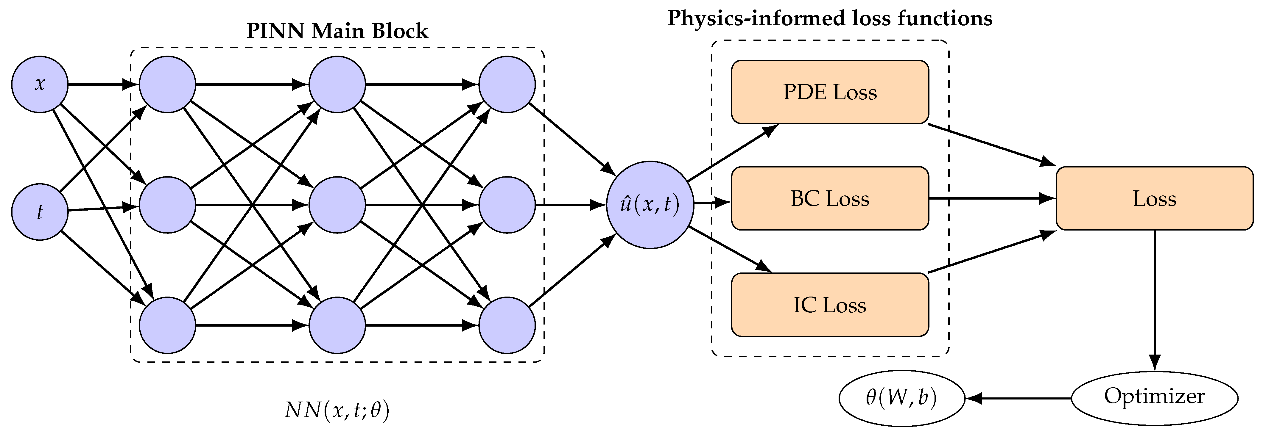
Using the training samples, which include both the interior and boundary points of the domain, we apply the loss function to enforce Robin boundary conditions. The schematic diagram in Figure 1 shows the training approach used to solve the Advection–Diffusion–Reaction Equation (1). The Glorot normal distribution was used to initialize the PINN model, and a learning rate of ${10}^{-3}$ was used to optimize it. We investigated different activation function combinations, optimization techniques, and neural network architectures designed for the linear ADR equation under boundary constraints to identify the optimal setup. To evaluate the ability of the model to predict during the training phase, the ground truth values $u(x_k,t_k)$ were compared to the corresponding network predictions $u(x_k,t_k)$ for every test scenario. This comparison allowed us to analyze the model’s performance and refine our approach iteratively. By adjusting parameters and tuning the architecture based on the prediction errors, we aimed to enhance the accuracy and robustness of our predictions in complex scenarios. The Automatica studies [20,21] contribute important conceptual guidance for improving the trainability of Physics-Informed Neural Networks by showing how difficult PDE features should be reformulated and constrained to ensure stability. In particular, their PDE-based treatment of delays and coupled dynamics demonstrates that complex non-local or memory effects can be handled more effectively by introducing auxiliary PDE states rather than learning them implicitly, a strategy that directly reduces stiffness and optimization difficulty in PINN training.

4. The Crank–Nicolson Finite Difference Method

The Crank–Nicolson Finite Difference Method, developed by John Crank and Phyllis Nicolson in the 1940s [22], is used to solve PDEs. It is an implicit second-order method in time. This method does not impose restrictions on the time-step size for stability, making it unconditionally stable. However, being implicit, it requires solving a system of linear equations at each time step, which can increase computational cost.

4.1. Mathematical Representation of CNFDM

The algorithm for the approximation of $u,u_t,u_x$ and $u_{xx}$ is given as follows:

$$\begin{array}{c}\hfill \left\{\begin{array}{c}{\displaystyle u\approx \frac{u_m^n+u_m^{n+1}}{2},}\hfill \\ {\displaystyle \frac{\partial u}{\partial t}\approx \frac{u_m^{n+1}-u_m^n}{\Delta t},}\hfill \\ {\displaystyle \frac{\partial u}{\partial x}\approx \frac{u_{m+1}^n-u_{m-1}^n+u_{m+1}^{n+1}-u_{m-1}^{n+1}}{4\Delta x},}\hfill \\ {\displaystyle \frac{{\partial }^{2}u}{\partial x^2}\approx \frac{u_{m+1}^n-2u_m^n+u_{m-1}^n+u_{m+1}^{n+1}-2u_m^{n+1}+u_{m-1}^{n+1}}{2\Delta x^2},}\hfill \end{array}\right.\end{array}$$

(16)

where $\Delta x=0.1$ and $\Delta t=0.001$ represent the spatial step sizes and the temporal steps, respectively.

4.1.1. Consistency Analysis for the 1D ADR Equation

$$\begin{array}{c}\hfill {\displaystyle \frac{\partial u}{\partial t}}+5{\displaystyle \frac{\partial u}{\partial x}}-{\displaystyle \frac{{\partial }^{2}u}{\partial x^2}}+u=0,\end{array}$$

(17)

By substituting the approximations from Equation (16) into the 1D ADR equation Equation (17), we obtain the following.

$$\begin{array}{cc}\hfill {\displaystyle \frac{1}{\Delta t}}\left(u_m^{n+1}-u_m^n\right)& +{\displaystyle \frac{5}{4\Delta x}}\left(u_{m+1}^n-u_{m-1}^n+u_{m+1}^{n+1}-u_{m-1}^{n+1}\right)\hfill \\ \hfill & -{\displaystyle \frac{1}{2{(\Delta x)}^2}}\left(u_{m+1}^n-2u_m^n+u_{m-1}^n+u_{m+1}^{n+1}-2u_m^{n+1}+u_{m-1}^{n+1}\right)+{\displaystyle \frac{1}{2}}\left(u_m^{n+1}+u_m^n\right)=0,\hfill \end{array}$$

Grouping the like terms:

$$\begin{array}{cc}\hfill & \left({\displaystyle \frac{1}{\Delta t}}+{\displaystyle \frac{1}{2}}+{\displaystyle \frac{1}{{(\Delta x)}^2}}\right)u_m^{n+1}-\left({\displaystyle \frac{5}{4\Delta x}}+{\displaystyle \frac{1}{2{(\Delta x)}^2}}\right)u_{m-1}^{n+1}-\left(-{\displaystyle \frac{5}{4\Delta x}}+{\displaystyle \frac{1}{2{(\Delta x)}^2}}\right)u_{m+1}^{n+1}=\hfill \\ & \left({\displaystyle \frac{1}{2{(\Delta x)}^2}}-{\displaystyle \frac{5}{4\Delta x}}\right)u_{m+1}^n+\left({\displaystyle \frac{1}{\Delta t}}-{\displaystyle \frac{1}{{(\Delta x)}^2}}-{\displaystyle \frac{1}{2}}\right)u_m^n+\left({\displaystyle \frac{5}{4\Delta x}}+{\displaystyle \frac{1}{2{(\Delta x)}^2}}\right)u_{m-1}^n,\hfill \end{array}$$

(18)

Let

$$\begin{array}{c}\hfill \left\{\begin{array}{c}{\displaystyle P_1=\frac{1}{\Delta t}+\frac{1}{{(\Delta x)}^2}+\frac{1}{2},}\hfill \\ {\displaystyle P_2=\frac{5}{4\Delta x}+\frac{1}{2{(\Delta x)}^2},}\hfill \\ {\displaystyle P_3=\frac{1}{2{(\Delta x)}^2}-\frac{5}{4\Delta x},}\hfill \\ {\displaystyle P_4=\frac{1}{\Delta t}-\frac{1}{{(\Delta x)}^2}-\frac{1}{2}.}\hfill \end{array}\right.\end{array}$$

(19)

By substituting Equation (19) into Equation (18), we obtain the following scheme:

$$\begin{array}{cc}\hfill & -P_3{u}_{m+1}^{n+1}+P_1{u}_m^{n+1}-P_2{u}_{m-1}^{n+1}=P_3{u}_{m+1}^n+P_4{u}_m^n+P_2{u}_{m-1}^n.\hfill \end{array}$$

(20)

For m = 1, 2,…, M − 1, the scheme can be represented as a tri diagonal matrix system for each time step:

$$A{\mathbf{u}}^{n+1}=B{\mathbf{u}}^n,$$

(21)

where

$${\mathbf{u}}^{n+1}=\left[\begin{array}{c}{u}_1^{n+1}\\ u_2^{n+1}\\ ⋮\\ u_{M-1}^{n+1}\end{array}\right],{\mathbf{u}}^n=\left[\begin{array}{c}{u}_1^n\\ u_2^n\\ ⋮\\ u_{M-1}^n\end{array}\right].$$

and

$$A=\left[\begin{array}{ccccc}{P}_1& -P_3& 0& \cdots & 0\\ -P_2& P_1& -P_3& \cdots & 0\\ 0& -P_2& P_1& \cdots & 0\\ ⋮& ⋮& ⋮& \ddots & -P_3\\ 0& 0& 0& -P_2& P_1\end{array}\right],B=\left[\begin{array}{ccccc}{P}_4& P_3& 0& \cdots & 0\\ P_2& P_4& P_3& \cdots & 0\\ 0& P_2& P_4& \cdots & 0\\ ⋮& ⋮& ⋮& \ddots & P_3\\ 0& 0& 0& P_2& P_4\end{array}\right].$$

We use Taylor’s expansion to investigate the consistency at the mesh point $(x,t)=(x_m,t_n)$.

$$\begin{array}{c}\hfill \left\{\begin{array}{cc}{u}_m^{n+1}\hfill & \approx u+\Delta t{\displaystyle \frac{\partial u}{\partial t}}+{\displaystyle \frac{{(\Delta t)}^2}{2}}{\displaystyle \frac{{\partial }^{2}u}{\partial t^2}}+{\displaystyle \frac{{(\Delta t)}^3}{6}}{\displaystyle \frac{{\partial }^{3}u}{\partial t^3}}+{\displaystyle \frac{{(\Delta t)}^4}{24}}{\displaystyle \frac{{\partial }^{4}u}{\partial t^4}}+\cdots \hfill \\ u_{m-1}^n\hfill & \approx u-\Delta x{\displaystyle \frac{\partial u}{\partial x}}+{\displaystyle \frac{{(\Delta x)}^2}{2}}{\displaystyle \frac{{\partial }^{2}u}{\partial x^2}}-{\displaystyle \frac{{(\Delta x)}^3}{6}}{\displaystyle \frac{{\partial }^{3}u}{\partial x^3}}+{\displaystyle \frac{{(\Delta x)}^4}{24}}{\displaystyle \frac{{\partial }^{4}u}{\partial x^4}}+\cdots \hfill \\ u_{m+1}^n\hfill & \approx u+\Delta x{\displaystyle \frac{\partial u}{\partial x}}+{\displaystyle \frac{{(\Delta x)}^2}{2}}{\displaystyle \frac{{\partial }^{2}u}{\partial x^2}}+{\displaystyle \frac{{(\Delta x)}^3}{6}}{\displaystyle \frac{{\partial }^{3}u}{\partial x^3}}+{\displaystyle \frac{{(\Delta x)}^4}{24}}{\displaystyle \frac{{\partial }^{4}u}{\partial x^4}}+\cdots \hfill \\ u_{m+1}^{n+1}\hfill & \approx u+\Delta t{\displaystyle \frac{\partial u}{\partial t}}+\Delta x{\displaystyle \frac{\partial u}{\partial x}}+{\displaystyle \frac{{(\Delta x)}^2}{2}}{\displaystyle \frac{{\partial }^{2}u}{\partial x^2}}+(\Delta t\Delta x){\displaystyle \frac{{\partial }^{2}u}{\partial t\partial x}}+{\displaystyle \frac{{(\Delta t)}^2}{2}}{\displaystyle \frac{{\partial }^{2}u}{\partial t^2}}+\cdots \hfill \\ u_{m-1}^{n+1}\hfill & \approx u+\Delta t{\displaystyle \frac{\partial u}{\partial t}}-\Delta x{\displaystyle \frac{\partial u}{\partial x}}+{\displaystyle \frac{{(\Delta x)}^2}{2}}{\displaystyle \frac{{\partial }^{2}u}{\partial x^2}}-(\Delta t\Delta x){\displaystyle \frac{{\partial }^{2}u}{\partial t\partial x}}+{\displaystyle \frac{{(\Delta t)}^2}{2}}{\displaystyle \frac{{\partial }^{2}u}{\partial t^2}}+\cdots \hfill \end{array}\right.\end{array}$$

(22)

By substituting Equation (22) into Equation (20), we obtain the following:

$$\begin{array}{cc}\hfill & -P_3\left(u+\Delta t{\displaystyle \frac{\partial u}{\partial t}}+\Delta x{\displaystyle \frac{\partial u}{\partial x}}+{(\Delta x)}^2{\displaystyle \frac{{\partial }^{2}u}{\partial x^2}}+(\Delta t\Delta x){\displaystyle \frac{{\partial }^{2}u}{\partial t\partial x}}+{\displaystyle \frac{{(\Delta t)}^2}{2}}{\displaystyle \frac{{\partial }^{2}u}{\partial t^2}}+\dots \right)\hfill \\ \hfill & +P_1\left(u+\Delta t{\displaystyle \frac{\partial u}{\partial t}}+{\displaystyle \frac{{(\Delta t)}^2}{2}}{\displaystyle \frac{{\partial }^{2}u}{\partial t^2}}+{\displaystyle \frac{{(\Delta t)}^3}{6}}{\displaystyle \frac{{\partial }^{3}u}{\partial t^3}}+{\displaystyle \frac{{(\Delta t)}^4}{24}}{\displaystyle \frac{{\partial }^{4}u}{\partial t^4}}+\dots \right)\hfill \\ \hfill & -P_2\left(u+\Delta t{\displaystyle \frac{\partial u}{\partial t}}-\Delta x{\displaystyle \frac{\partial u}{\partial x}}+{(\Delta x)}^2{\displaystyle \frac{{\partial }^{2}u}{\partial x^2}}-(\Delta t\Delta x){\displaystyle \frac{{\partial }^{2}u}{\partial t\partial x}}+{\displaystyle \frac{{(\Delta t)}^2}{2}}{\displaystyle \frac{{\partial }^{2}u}{\partial t^2}}+\dots \right)\hfill \\ \hfill & =P_3\left(u+\Delta x{\displaystyle \frac{\partial u}{\partial x}}+{\displaystyle \frac{{(\Delta x)}^2}{2}}{\displaystyle \frac{{\partial }^{2}u}{\partial x^2}}+{\displaystyle \frac{{(\Delta x)}^3}{6}}{\displaystyle \frac{{\partial }^{3}u}{\partial x^3}}+{\displaystyle \frac{{(\Delta x)}^4}{24}}{\displaystyle \frac{{\partial }^{4}u}{\partial x^4}}+\dots \right)\hfill \\ \hfill & +P_{4}u+P_2\left(u_m^n-\Delta x{\displaystyle \frac{\partial u}{\partial x}}+{\displaystyle \frac{{(\Delta x)}^2}{2}}{\displaystyle \frac{{\partial }^{2}u}{\partial x^2}}-{\displaystyle \frac{{(\Delta x)}^3}{6}}{\displaystyle \frac{{\partial }^{3}u}{\partial x^3}}+{\displaystyle \frac{{(\Delta x)}^4}{24}}{\displaystyle \frac{{\partial }^{4}u}{\partial x^4}}+\dots \right)\hfill \end{array}$$

(23)

Grouping like terms yield the following equation:

$$\begin{array}{cc}\hfill & (-2P_3+P_1-2P_2-P_4)u+(P_1-P_2-P_3)\Delta t{\displaystyle \frac{\partial u}{\partial t}}+(P_1-P_2-P_3)\left({\displaystyle \frac{{(\Delta t)}^2}{2}}\right){\displaystyle \frac{{\partial }^{2}u}{\partial t^2}}\hfill \\ \hfill & +P_1\left({\displaystyle \frac{{(\Delta t)}^3}{6}}\right){\displaystyle \frac{{\partial }^{3}u}{\partial t^3}}+P_1\left({\displaystyle \frac{{(\Delta t)}^4}{24}}\right){\displaystyle \frac{{\partial }^{4}u}{\partial t^4}}\hfill \\ \hfill & +(2P_2-2P_3)\Delta x{\displaystyle \frac{\partial u}{\partial x}}+(-2P_2-2P_3)\left({\displaystyle \frac{{(\Delta x)}^2}{2}}\right){\displaystyle \frac{{\partial }^{2}u}{\partial x^2}}\hfill \\ \hfill & +(P_2-P_3)\Delta t\Delta x{\displaystyle \frac{{\partial }^{2}u}{\partial t\partial x}}+(P_2-P_3)\left({\displaystyle \frac{{(\Delta x)}^3}{6}}\right){\displaystyle \frac{{\partial }^{3}u}{\partial x^3}}\hfill \\ \hfill & +(-P_3-P_2)\left({\displaystyle \frac{{(\Delta x)}^4}{24}}\right){\displaystyle \frac{{\partial }^{4}u}{\partial x^4}}=0.\hfill \end{array}$$

(24)

Further simplification of Equation (24) leads to the following equation:

$$\begin{array}{cc}\hfill & u+\left({\displaystyle \frac{1}{\Delta t}}+{\displaystyle \frac{1}{2}}\right)\Delta t{\displaystyle \frac{\partial u}{\partial t}}+\left({\displaystyle \frac{1}{\Delta t}}+{\displaystyle \frac{1}{2}}\right){\displaystyle \frac{{(\Delta t)}^2}{2}}{\displaystyle \frac{{\partial }^{2}u}{\partial t^2}}+\left({\displaystyle \frac{1}{\Delta t}}+{\displaystyle \frac{1}{2}}+{\displaystyle \frac{1}{\Delta x^2}}\right){\displaystyle \frac{{(\Delta t)}^3}{6}}{\displaystyle \frac{{\partial }^{3}u}{\partial t^3}}+\hfill \\ & \left({\displaystyle \frac{1}{\Delta t}}+{\displaystyle \frac{1}{2}}+{\displaystyle \frac{1}{\Delta x^2}}\right){\displaystyle \frac{{(\Delta t)}^4}{24}}{\displaystyle \frac{{\partial }^{4}u}{\partial t^4}}+\left({\displaystyle \frac{5}{\Delta x}}\right)\Delta x{\displaystyle \frac{\partial u}{\partial x}}+\left(-{\displaystyle \frac{2}{\Delta x^2}}\right){\displaystyle \frac{{(\Delta x)}^2}{2}}{\displaystyle \frac{{\partial }^{2}u}{\partial x^2}}\hfill \\ \hfill & +\left({\displaystyle \frac{5}{2\Delta x}}\right)\left(\Delta t\Delta x\right){\displaystyle \frac{{\partial }^{2}u}{\partial t\partial x}}+\left({\displaystyle \frac{5}{2\Delta x}}\right){\displaystyle \frac{{(\Delta x)}^3}{6}}{\displaystyle \frac{{\partial }^{3}u}{\partial x^3}}+\left(-{\displaystyle \frac{1}{\Delta x^2}}\right){\displaystyle \frac{{(\Delta x)}^4}{24}}{\displaystyle \frac{{\partial }^{4}u}{\partial x^4}}=0\hfill \end{array}$$

(25)

Further simplification of the above equation leads to the following equation:

$$\begin{array}{cc}\hfill & u+\left(1+{\displaystyle \frac{\Delta t}{2}}\right){\displaystyle \frac{\partial u}{\partial t}}+\left({\displaystyle \frac{\Delta t}{2}}+{\displaystyle \frac{\Delta t^2}{2}}\right){\displaystyle \frac{{\partial }^{2}u}{\partial t^2}}+\left({\displaystyle \frac{\Delta t^2}{6}}+{\displaystyle \frac{\Delta t^3}{12}}+{\displaystyle \frac{\Delta t^3}{6\Delta x^2}}\right){\displaystyle \frac{{\partial }^{3}u}{\partial t^3}}+\left({\displaystyle \frac{1\Delta t^3}{24}}+{\displaystyle \frac{\Delta t^4}{48}}+{\displaystyle \frac{\Delta t^4}{24\Delta x^2}}\right){\displaystyle \frac{{\partial }^{4}u}{\partial t^4}}\hfill \\ \hfill & +5{\displaystyle \frac{\partial u}{\partial x}}-{\displaystyle \frac{{\partial }^{2}u}{\partial x^2}}+\left({\displaystyle \frac{5\Delta t}{2}}\right){\displaystyle \frac{{\partial }^{2}u}{\partial t\partial x}}+\left({\displaystyle \frac{5\Delta x^2}{12}}\right){\displaystyle \frac{{\partial }^{3}u}{\partial x^3}}+\left(-{\displaystyle \frac{\Delta x^2}{24}}\right){\displaystyle \frac{{\partial }^{4}u}{\partial x^4}}=0,\hfill \end{array}$$

(26)

When $\Delta t\to 0$ and $\Delta x\to 0$, Equation (26) is not consistent, and hence we set $\Delta t=\Delta x$, to obtain:

$$\begin{array}{cc}\hfill & u+\left(1+{\displaystyle \frac{\Delta t}{2}}\right){\displaystyle \frac{\partial u}{\partial t}}+\left({\displaystyle \frac{\Delta t}{2}}+{\displaystyle \frac{\Delta t^2}{2}}\right){\displaystyle \frac{{\partial }^{2}u}{\partial t^2}}+\left({\displaystyle \frac{\Delta t^2}{6}}+{\displaystyle \frac{\Delta t^3}{12}}+{\displaystyle \frac{\Delta t^3}{6\Delta t^2}}\right){\displaystyle \frac{{\partial }^{3}u}{\partial t^3}}+\left({\displaystyle \frac{\Delta t^3}{24}}+{\displaystyle \frac{\Delta t^4}{48}}+{\displaystyle \frac{\Delta t^2}{24}}\right){\displaystyle \frac{{\partial }^{4}u}{\partial t^4}}\hfill \\ \hfill & +5{\displaystyle \frac{\partial u}{\partial x}}-{\displaystyle \frac{{\partial }^{2}u}{\partial x^2}}+\left({\displaystyle \frac{5\Delta t}{2}}\right){\displaystyle \frac{{\partial }^{2}u}{\partial t\partial x}}+\left({\displaystyle \frac{5\Delta t^2}{12}}\right){\displaystyle \frac{{\partial }^{3}u}{\partial x^3}}+\left(-{\displaystyle \frac{\Delta t^2}{24}}\right){\displaystyle \frac{{\partial }^{4}u}{\partial x^4}}=0,\hfill \end{array}$$

(27)

When $\Delta t\to 0$, we obtain:

$$\begin{array}{c}\hfill u+{\displaystyle \frac{\partial u}{\partial t}}+5{\displaystyle \frac{\partial u}{\partial x}}-{\displaystyle \frac{{\partial }^{2}u}{\partial x^2}}=0,\end{array}$$

(28)

Therefore, the original ADR Equation (17) is derived from the scheme and it is evident that the consistency of the scheme is conditional on the relationship $\Delta t=\Delta x$.

4.1.2. Stability Analysis

In this section, we analyze the behavior of equilibria or steady state. These are specific conditions where the system remains unchanged over time. Stability analysis helps determine if these equilibria are stable, meaning that the system returns to the equilibrium after being disturbed, or being unstable, in which case it moves further away from the equilibrium. The von Neumann stability analysis is used to determine the stability region of finite difference methods. To begin the analysis, we define the error between the exact and numerical solutions as

$$\begin{array}{cc}\hfill z_m^n& \approx {\tilde{u}}_m^n-u_m^n={\xi }^n{e}^{ikm\Delta x},\hfill \end{array}$$

(29)

where ${\tilde{u}}_m^n$ and $u_m^n$ represents the exact solution and the numerical solution, respectively. $\xi$ is the amplification factor, and $\omega =k\Delta x$ is the phase angle, which varies within the interval $[-\pi ,\pi ]$.

$$\begin{array}{c}\hfill \left\{\begin{array}{cc}{u}_m^n\hfill & ={\xi }^n{e}^{ikm\Delta x},\hfill \\ u_{m-1}^{n+1}\hfill & ={\xi }^{n+1}{e}^{ik(m-1)\Delta x},\hfill \\ u_m^{n+1}\hfill & ={\xi }^{n+1}{e}^{ikm\Delta x}\hfill \\ u_{m+1}^{n+1}\hfill & ={\xi }^{n+1}{e}^{ik(m+1)\Delta x},\hfill \\ u_{m-1}^n\hfill & ={\xi }^n{e}^{ik(m-1)\Delta x},\hfill \\ u_{m+1}^n\hfill & ={\xi }^n{e}^{ik(m+1)\Delta x}.\hfill \end{array}\right.\end{array}$$

(30)

By substituting Equation (30) into the scheme defined by Equation (20), we obtain the following:

$$\begin{array}{cc}\hfill & -P_3{\xi }^{n+1}{e}^{ik(m+1)\Delta x}+P_1{\xi }^{n+1}{e}^{ik\left(m\right)\Delta x}-P_2{\xi }^{n+1}{e}^{ik(m-1)\Delta x}=P_3{\xi }^n{e}^{ik(m+1)\Delta x}+P_4{\xi }^n{e}^{ikm\Delta x}\hfill \\ \hfill & +P_2{\xi }^n{e}^{ik(m-1)\Delta x},\hfill \end{array}$$

(31)

$$\begin{array}{cc}\hfill & {\xi }^{n+1}{e}^{i\omega m}\left(-P_3{e}^{i\omega }+P_1-P_2{e}^{-i\omega }\right)={\xi }^n{e}^{i\omega m}\left(P_3{e}^{i\omega }+P_4+P_2{e}^{-i\omega }\right).\hfill \end{array}$$

(32)

By simplifying Equation (32), we obtain the following Equation:

$$\begin{array}{cc}\hfill & {\xi }^{n+1}\left(-P_3{e}^{i\omega }+P_1-P_2{e}^{-i\omega }\right)={\xi }^n\left(P_3{e}^{i\omega }+P_4+P_2{e}^{-i\omega }\right).\hfill \end{array}$$

(33)

By simplifying Equation (33), we obtain the following Equation:

$$\begin{array}{cc}\hfill & \xi \left(-P_3{e}^{i\omega }+P_1-P_2{e}^{-i\omega }\right)=\left(P_3{e}^{i\omega }+P_4+P_2{e}^{-i\omega }\right),\hfill \end{array}$$

(34)

$$\begin{array}{c}\hfill \xi ={\displaystyle \frac{P_3{e}^{i\omega }+P_4+P_2{e}^{-i\omega }}{-P_3{e}^{i\omega }+P_1-P_2{e}^{-i\omega }}}.\end{array}$$

(35)

It follows from Euler’s formula that:

$$\begin{array}{c}\hfill e^{i\theta }=cos\left(\theta \right)+isin\left(\theta \right).\end{array}$$

(36)

Therefore, Equation (35) yields:

$$\begin{array}{c}\hfill \xi ={\displaystyle \frac{P_3(cos\left(\omega \right)+isin\left(\omega \right))+P_4+P_2(cos\left(\omega \right)-isin\left(\omega \right))}{-P_3(cos\left(\omega \right)+isin\left(\omega \right))+P_1-P_2(cos\left(\omega \right)-isin\left(\omega \right))}},\end{array}$$

(37)

$$\begin{array}{c}\hfill \xi ={\displaystyle \frac{\left(P_4+(P_3+P_2)cos\left(\omega \right)+(P_3-P_2)isin\left(\omega \right)\right)}{\left(P_1-(P_3+P_2)cos\left(\omega \right)-i(P_3-P_2)sin\left(\omega \right)\right)}}.\end{array}$$

(38)

We simplify the key combinations of $P_2$ and $P_3$:

$$\begin{array}{c}\hfill \left\{\begin{array}{cc}{P}_2+P_3\hfill & =\left({\displaystyle \frac{1}{2(\Delta x^2}}-{\displaystyle \frac{5}{4\Delta x}}\right)+\left({\displaystyle \frac{5}{4\Delta x}}+{\displaystyle \frac{1}{2{(\Delta x)}^2}}\right)\hfill \\ \hfill & ={\displaystyle \frac{1}{{(\Delta x)}^2}}.\hfill \\ P_3-P_2\hfill & =\left({\displaystyle \frac{1}{2(\Delta x^2}}-{\displaystyle \frac{5}{4\Delta x}}\right)-\left({\displaystyle \frac{5}{4\Delta x}}+{\displaystyle \frac{1}{2{(\Delta x)}^2}}\right)\hfill \\ \hfill & =-{\displaystyle \frac{5}{2\Delta x}}.\hfill \end{array}\right.\end{array}$$

(39)

By substituting Equation (39) into Equation (38) we obtain the following:

$$\begin{array}{c}\hfill \xi ={\displaystyle \frac{\left(\frac{1}{\Delta t}-\frac{1}{2}-\frac{1}{{(\Delta x)}^2}(1-cos\left(\omega \right)\right)-i\frac{5}{2\Delta x}sin\left(\omega \right)}{\left(\frac{1}{\Delta t}+\frac{1}{2}+\frac{1}{{(\Delta x)}^2}(1-cos\left(\omega \right)\right)+i\frac{5}{2\Delta x}sin\left(\omega \right)}}.\end{array}$$

(40)

The von Neumann stability condition is such that

$${\left|\xi \right|}^2\le 1,$$

that is,

$$\begin{array}{c}\hfill {\left|\xi \right|}^2={\left|{\displaystyle \frac{\left(\frac{1}{\Delta t}-\frac{1}{2}-\frac{1}{{(\Delta x)}^2}(1-cos\left(\omega \right)\right)-i\frac{5}{2\Delta x}sin\left(\omega \right)}{\left(\frac{1}{\Delta t}+\frac{1}{2}+\frac{1}{{(\Delta x)}^2}(1-cos\left(\omega \right)\right)+i\frac{5}{2\Delta x}sin\left(\omega \right)}}\right|}^2\le 1,\end{array}$$

(41)

$$\begin{array}{c}\hfill {\displaystyle \frac{{\left(\frac{1}{\Delta t}-\frac{1}{2}-\frac{1}{{(\Delta x)}^2}(1-cos\left(\omega \right))\right)}^2+{\left(\frac{5\sin \left(\omega \right)}{2\Delta x}\right)}^2}{{\left(\frac{1}{\Delta t}+\frac{1}{2}+\frac{1}{{(\Delta x)}^2}(1-cos\left(\omega \right))\right)}^2+{\left(\frac{5\sin \left(\omega \right)}{2\Delta x}\right)}^2}}\le 1,\end{array}$$

(42)

Using the half-angle identity for $1-cos\left(\omega \right)=2si{n}^2\left({\displaystyle \frac{\omega }{2}}\right)$, we obtain the following:

$$\begin{array}{c}\hfill {\displaystyle \frac{{\left(\frac{1}{\Delta t}-\frac{1}{2}-\frac{2}{{(\Delta x)}^2}si{n}^2\left(\frac{\omega }{2}\right)\right)}^2+{\left(\frac{5\sin \left(\omega \right)}{2\Delta x}\right)}^2}{{\left(\frac{1}{\Delta t}+\frac{1}{2}+\frac{2}{{(\Delta x)}^2}si{n}^2\left(\frac{\omega }{2}\right)\right)}^2+{\left(\frac{5\sin \left(\omega \right)}{2\Delta x}\right)}^2}}\le 1,\end{array}$$

(43)

Let

$$\begin{array}{c}\hfill \left\{\begin{array}{c}\varphi ={\displaystyle \frac{1}{\Delta t}}-{\displaystyle \frac{1}{2}}-{\displaystyle \frac{2}{{(\Delta x)}^2}}(si{n}^2\left({\displaystyle \frac{\omega }{2}}\right)\hfill \\ \psi ={\displaystyle \frac{5\sin \left(\omega \right)}{2\Delta x}}\hfill \\ \mu ={\displaystyle \frac{1}{\Delta t}}+{\displaystyle \frac{1}{2}}+{\displaystyle \frac{2}{{(\Delta x)}^2}}(si{n}^2\left({\displaystyle \frac{\omega }{2}}\right),\hfill \end{array}\right.\end{array}$$

(44)

By substituting Equation (44) into Equation (43) we obtain the following:

$$\begin{array}{cc}\hfill & {\displaystyle \frac{{\varphi }^2+{\psi }^2}{{\mu }^2+{\psi }^2}}\le 1,\hfill \end{array}$$

(45)

Further simplification of Equation (45) leads to the following equation:

$$\begin{array}{cc}\hfill & {\varphi }^2+{\psi }^2\le {\mu }^2+{\psi }^2\hfill \\ \hfill & {\varphi }^2\le {\mu }^2\hfill \\ \hfill & {\mu }^2-{\varphi }^2\ge 0,\hfill \end{array}$$

(46)

By substituting Equation (44) into Equation (46) we obtain the following:

$$\begin{array}{c}\hfill {\left({\displaystyle \frac{1}{\Delta t}}+{\displaystyle \frac{1}{2}}-{\displaystyle \frac{2}{{(\Delta x)}^2}}(si{n}^2\left({\displaystyle \frac{\omega }{2}}\right)\right)}^2-{\left({\displaystyle \frac{1}{\Delta t}}-{\displaystyle \frac{1}{2}}+{\displaystyle \frac{2}{{(\Delta x)}^2}}(si{n}^2\left({\displaystyle \frac{\omega }{2}}\right)\right)}^2\ge 0\end{array}$$

(47)

By letting $\omega ={\displaystyle \frac{\pi }{2}}$, Equation (47) becomes:

$$\begin{array}{c}\hfill {\left({\displaystyle \frac{1}{\Delta t}}-{\displaystyle \frac{1}{2}}+{\displaystyle \frac{1}{{(\Delta x)}^2}}\right)}^2-{\left({\displaystyle \frac{1}{\Delta t}}+{\displaystyle \frac{1}{2}}-{\displaystyle \frac{1}{{(\Delta x)}^2}}\right)}^2\le 0,\end{array}$$

(48)

Further simplifications of Equation (48) lead to the following equation:

$$\begin{array}{c}\hfill {\displaystyle \frac{2}{\Delta t}}\left(1+{\displaystyle \frac{2}{{(\Delta x)}^2}}\right)\ge 0.\end{array}$$

(49)

Equation (49) holds under the conditions that $\Delta x\le \sqrt{2}$ and $\Delta t>0$. The CNFDM for the ADR equation is unconditionally stable under von Neumann analysis.

5. Results and Discussion

This section presents the comparative results of the numerical solutions obtained using PINNs and the CNFDM against the exact solution of the ADR equation. The comparisons focus on accuracy, error distribution, and the computational cost. The $L_2$ error was computed from the absolute errors reported in the last table before Section 5.1 using the root mean square definition $L_2=\sqrt{{\displaystyle \frac{1}{N}}{\sum }_{i=1}^N{\left(U_{pred}\left(x_i\right)-U_{exact}\left(x_i\right)\right)}^2}$. The error distribution refers to how these differences are spread across all observations. Understanding this distribution helps evaluate model assumptions, accuracy, and reliability. Computational cost denotes the amount of resources, such as time and memory, that an algorithm or model consumes during execution. Evaluating computational cost is essential for determining the efficiency of computational processes.

The PINNs code implementation began by defining the spatial and temporal domains and generating a mesh grid of points for training. The numerical tests in this study are performed using synthetic data generated from the analytical solution of the Advection–Diffusion–Reaction equation. A fully connected neural network was constructed with two hidden layers, each containing 80 neurons and using Tanh activation functions, which is elected because of its smoothness and differentiability, which are essential for Physics-Informed Neural Networks where derivatives of the network output must be computed accurately using automatic differentiation. Initial and boundary conditions are set up as tensors on the grid. The loss function $\left(L_{Total}\right)$ is defined as the sum of the PDE residual at collocation points $\left(L_{PDE}\right)$, the error at the initial condition $\left(L_{IC}\right)$, and errors at the left and right boundary conditions $(L_{Left-BC}$ and $L_{Right-BC})$. Training proceeds in two stages: First, Adam optimizer with a learning rate (lr) of 0.001 is applied for 9000 epochs to obtain a stable initial approximation, with the loss monitored every 1000 epochs. Then, the L-BFGS optimizer with a learning rate of 1.0 and strict gradient and convergence tolerances is used for fine tuning. After training, the network is evaluated on the full grid, the predicted values are reshaped to match the grid, and the absolute error is computed by comparing the predictions to exact values. This implementation was done on Google Colaboratory together with the CNFDM code.

The 2-D plots and the tables below visualize the comparison of the numerical solution obtained using the CNFDM and PINNs against the results from the exact solution at different time and space steps, respectively for better analysis (see

Table 1. Sensitivity analysis of the PINN architecture for the ADR problem.

Hidden Layers	Neurons per Layer	Activation	${\mathit{L}}_2$ Error	CPU Time
2	40	Tanh	$1.2\times {10}^{-3}$	1 h 20 min
2	80	Tanh	$6.8\times {10}^{-4}$	2 h 30 min
3	80	Tanh	$6.5\times {10}^{-4}$	3 h 40 min
2	80	ReLU	$2.4\times {10}^{-3}$	2 h 15 min

).

Sensitivity analysis demonstrated that the optimal PINN architecture (two layers, 80 neurons) achieved an $L_2$ error of $6.8\times {10}^{-4}$. Furthermore, it was observed that the Tanh activation function provided superior convergence over ReLU, reducing the $L_2$ error by approximately $71\%$ in identical architectures (see

Table 2. Mesh Convergence study for CNFDM.

$\Delta \mathit{x}$	${\mathit{L}}_2$ Error	Convergence Rate
$0.40$	$1.158878$	−
$0.20$	$0.181117$	$2.68$
$0.10$	$0.055470$	$1.71$
$0.05$	$0.017089$	$1.70$

).

A mesh refinement study was performed for the Crank–Nicolson Finite Difference Method using grid sizes $\Delta =0.40,0.20,0.10,0.05$. The numerical results show a convergence rate approaching two, confirming the expected second-order accuracy $(\Delta x^2+\Delta t^2)$ (see

Table 3. Training convergence for PINNs.

Collocation Points ${\mathit{N}}_{\mathit{f}}$	${\mathit{L}}_2$ Error	Convergence Rate
1000	$2.1\times {10}^{-3}$	−
2000	$1.3\times {10}^{-3}$	$0.69$
4000	$8.2\times {10}^{-4}$	$0.67$
8000	$6.8\times {10}^{-4}$	$0.27$

).

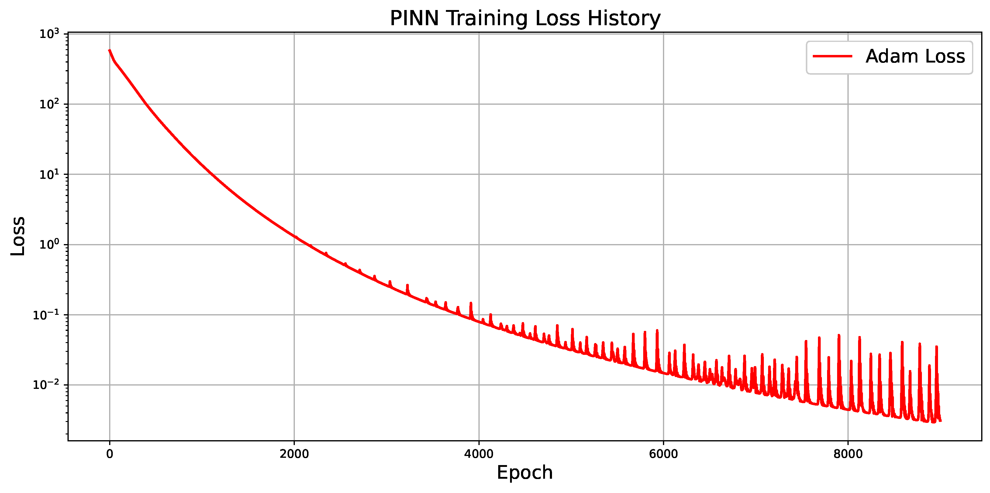
A training refinement study was performed for the PINN model by increasing the number of collocation points. The results show algebraic convergence with an empirical rate between $0.6$ and $0.8$, which is consistent with previously reported PINN training behaviour (see Figure 2).

The training loss history of the PINN used to solve the Advection–Diffusion–Reaction equation demonstrates a clear and stable convergence during the optimization process. Initially, the loss is relatively high, indicating a large discrepancy between the neural network predictions and the physical constraints imposed by the governing equation, boundary conditions, and initial conditions. As training progresses, a rapid decrease in the loss is observed during the early epochs, which suggests that the network quickly captures the dominant dynamics of the system governed by advection, diffusion, and reaction processes. In the intermediate training phase, the loss continues to decrease more gradually as the model refines the approximation and reduces the residuals of the governing partial differential equation at the collocation points. Minor oscillations appear in the later epochs, which can be attributed to the adaptive updates of the Adam optimizer and the complex nonlinear optimization landscape associated with the coupled physical processes. Nevertheless, the overall downward trend indicates that the PINN effectively learns a solution that satisfies the underlying physical laws. The final loss reaching the order of ${10}^{-3}$ suggests that the model achieves a high level of accuracy, demonstrating the capability of PINNs to approximate the solution of Advection–Diffusion–Reaction equations without relying on traditional mesh-based discretization methods (see

Table 4. $L_2$-norm for the CNFDM and PINNs techniques when solving ADR equation.

Position (x)	CNFDM ${\mathit{L}}_2$ Error	PINNs ${\mathit{L}}_2$ Error
0.0	$0.000000$	$2.19\times {10}^{-3}$
1.0	$1.49\times {10}^{-2}$	$3.08\times {10}^{-4}$
2.0	$1.02\times {10}^{-3}$	$5.19\times {10}^{-4}$
3.0	$6.39\times {10}^{-3}$	$4.89\times {10}^{-4}$
4.0	$3.09\times {10}^{-3}$	$4.61\times {10}^{-4}$
5.0	$1.53\times {10}^{-4}$	$1.400\times {10}^{-4}$
6.0	$4.69\times {10}^{-4}$	$3.40\times {10}^{-4}$
7.0	$2.06\times {10}^{-4}$	$3.26\times {10}^{-4}$
8.0	$1.01\times {10}^{-4}$	$2.93\times {10}^{-4}$
9.0	$7.6\times {10}^{-5}$	$2.71\times {10}^{-4}$
10.0	$2.2\times {10}^{-5}$	$1.89\times {10}^{-4}$

The PINNs demonstrate improved stability across the interior region.

).

5.1. Results for the CNFDM, PINNs and Exact Solutions at t = 0.085

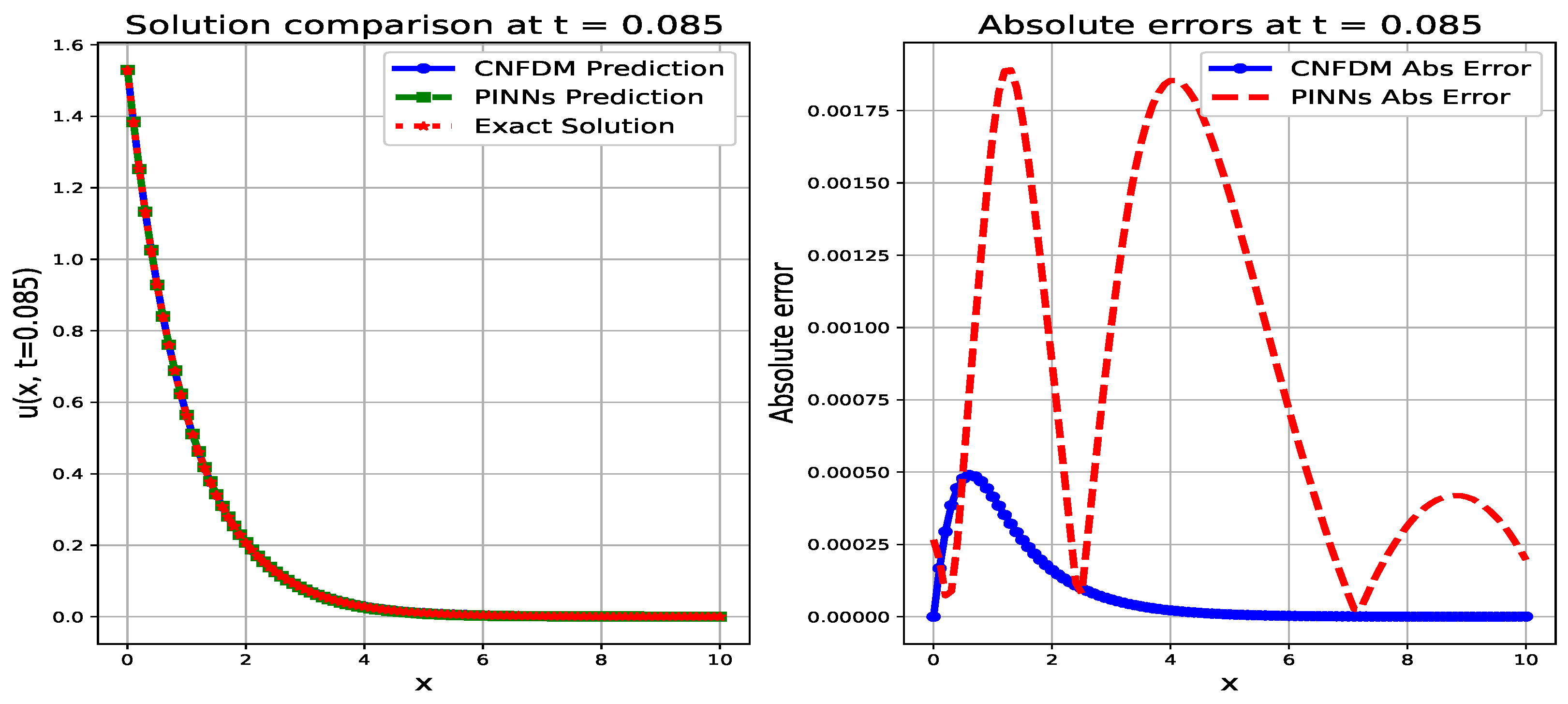
Figure 3 reveals a superior performance of CNFDM is maintained at $t=0.085$, and is more precise in terms of accuracy, with its maximum error being 0.000415 at $x=1.0$. The PINNs method is less accurate, with a higher maximum error of 0.001208 at $x=2.0$. The error distribution plot shows that the CNFDM absolute error is smaller and more contained, while the PINNs error is significantly larger and more widely distributed, with multiple high magnitude peaks, reinforcing the higher reliability and consistency of CNFDM at this later time step.

5.2. Results for the CNFDM, PINNs and Exact Solutions at t = 0.170

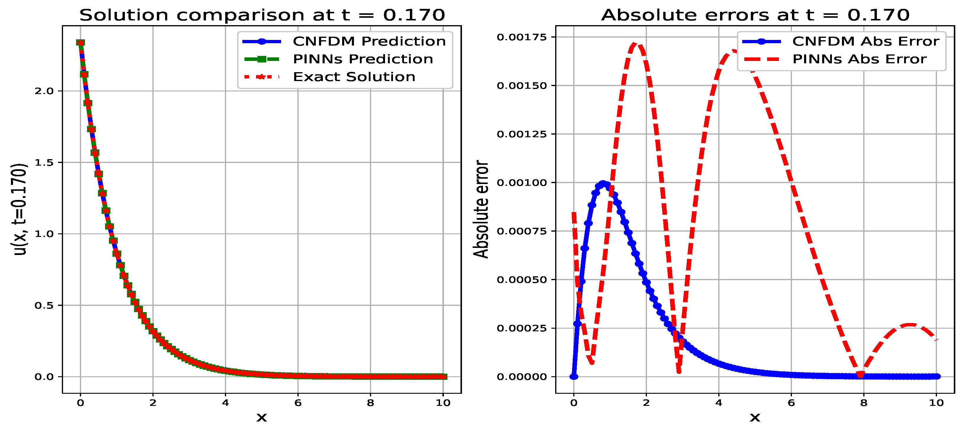
Figure 4 reveals that PINNs obtained a significantly lower maximum absolute error of 0.000875 (at $x=3.0$), slightly exceeding the CNFDM peak error of 0.000970 (at $x=1.0$), according to the comparison results for the solution at $t=0.170$. Additionally, the Absolute Error Plot’s error distribution shows that the PINNs’ error is more erratic and oscillatory throughout the domain, whereas the CNFDM error profile is smoother and more confined, indicating superior overall spatial consistency.

5.3. Results for the CNFDM, PINNs and Exact Solutions at t = 0.255

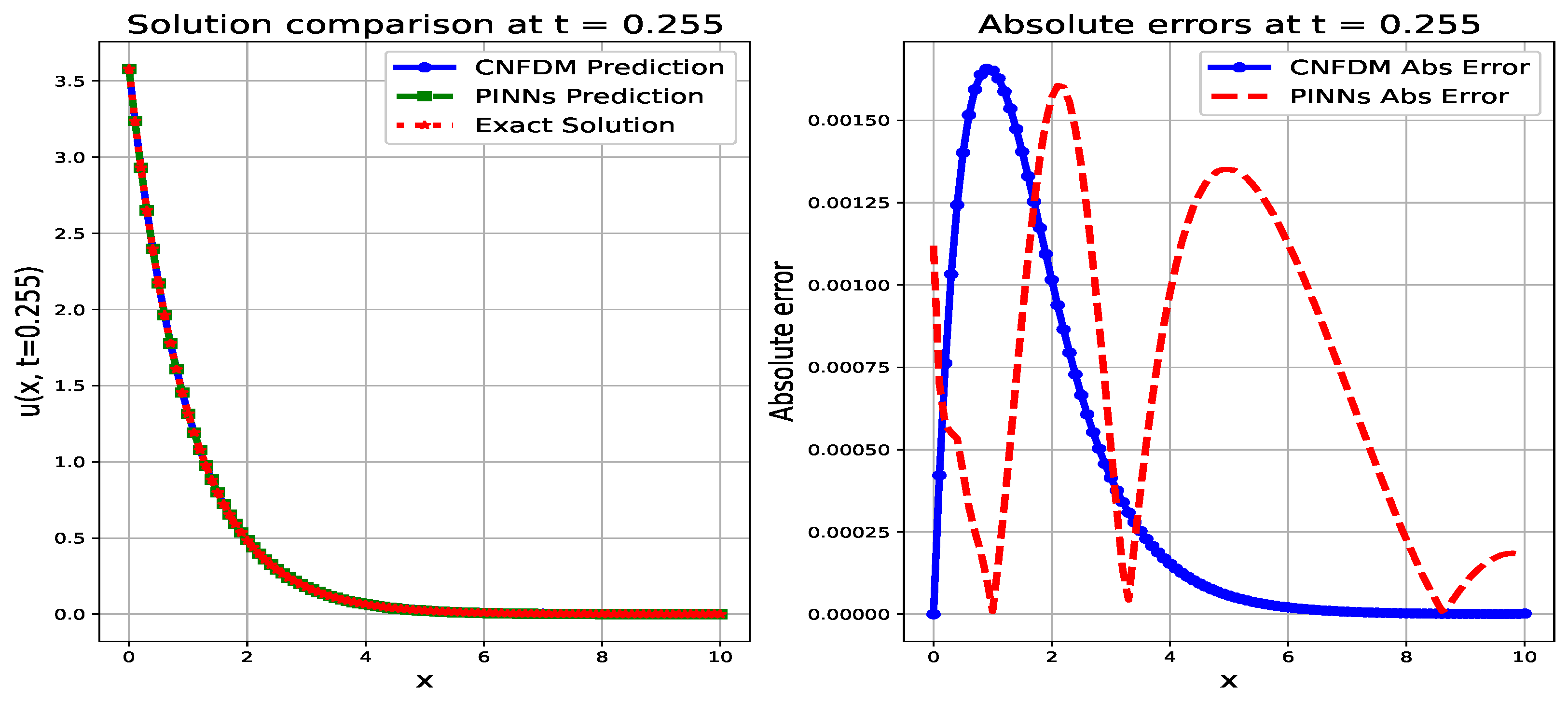
Figure 5 reveals that at the later time step of $t=0.255$, the performance gap in accuracy narrows and partially reverses. The CNFDM maximum error increases significantly to 0.001651 (at $x=1.0$), while the PINNs maximum error is lower at 0.000843 (at $x=3.0$). However, an analysis of the error distribution plot shows that the CNFDM error is highly concentrated into a single, large peak, whereas the PINNs error is lower at its peak but still highly non-uniform and oscillatory with multiple smaller peaks across the domain, suggesting less consistent spatial accuracy.

5.4. Results for the CNFDM, PINNs and Exact Solutions at t = 0.340

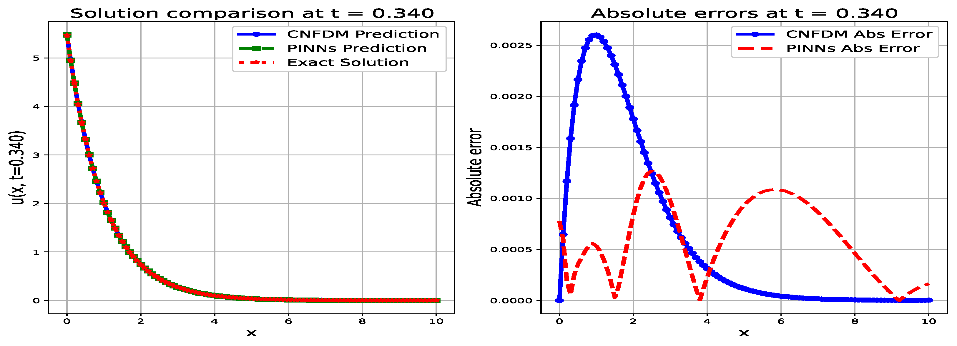
Figure 6 reveal that at $t=0.340$ the PINNs method achieved a lower maximum absolute error of 0.000727 (at $x=4.0$) compared to the CNFDM maximum error of 0.002601 (at $x=1.0$). However, an analysis of the error distribution plot reveals that while CNFDM error is highly concentrated in a single large peak, the PINNs absolute error is highly non-uniform and oscillatory with multiple peaks across the domain, suggesting CNFDM maintains a smoother and more consistent error profile overall.

5.5. Results for the CNFDM, PINNs and Exact Solutions at t = 0.425

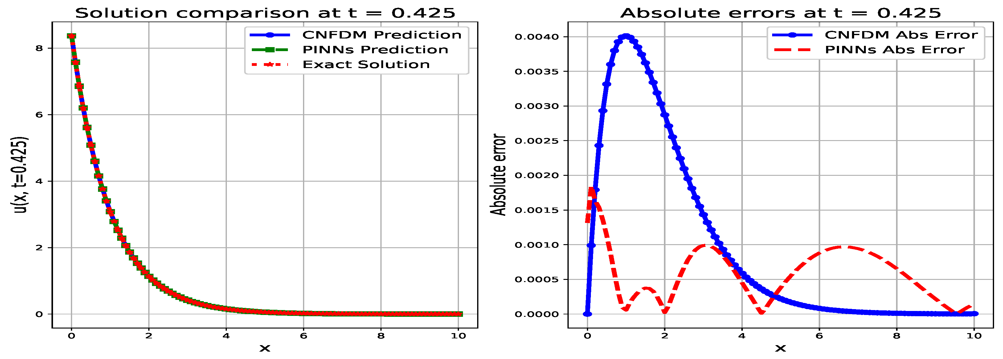
Figure 7 reveals that at $t=0.425$ the PINNs method achieved a significantly lower maximum absolute error than the CNFDM. The PINNs maximum error is 0.000736 (at $x=4.0$), which is much lower than the CNFDM maximum error of 0.004013 (at $x=1.0$). However, an analysis of the error distribution in the Absolute Error Plot shows a trade-off in consistency. The CNFDM error is highly concentrated in a single large peak near the boundary, while the PINNs absolute error, despite its lower peak magnitude, is still highly non-uniform and oscillatory, exhibiting multiple smaller peaks across the spatial domain.

5.6. Results for the CNFDM, PINNs and Exact Solutions at t = 0.510

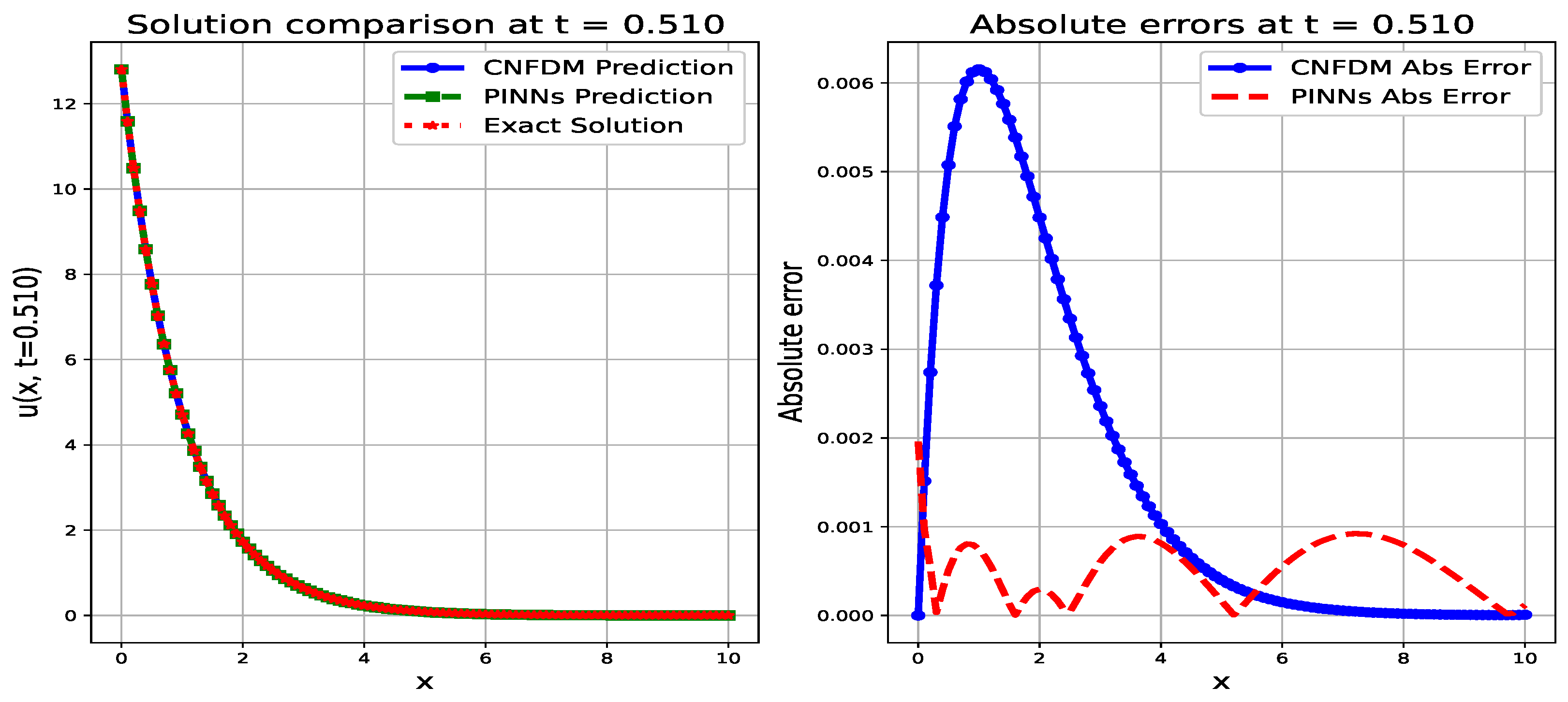
Figure 8 revealed that at $t=0.510$, the PINNs method was much more accurate than CNFDM. The biggest error for PINNs was only 0.000753, which is significantly smaller than CNFDM’s largest error of 0.006153. However, CNFDM maintains perfect accuracy at the boundary, with an error of 0.000000 at $x=0.0$, while PINNs have a small error of 0.000012 at that point. This divergence is visible in the error distribution plot, where the CNFDM error is highly concentrated into a single, very large peak near the boundary, while the PINNs absolute error, despite its lower peak magnitude, is highly non-uniform and oscillatory across the spatial domain.

5.7. Results for the CNFDM, PINNs and Exact Solutions at t = 0.595

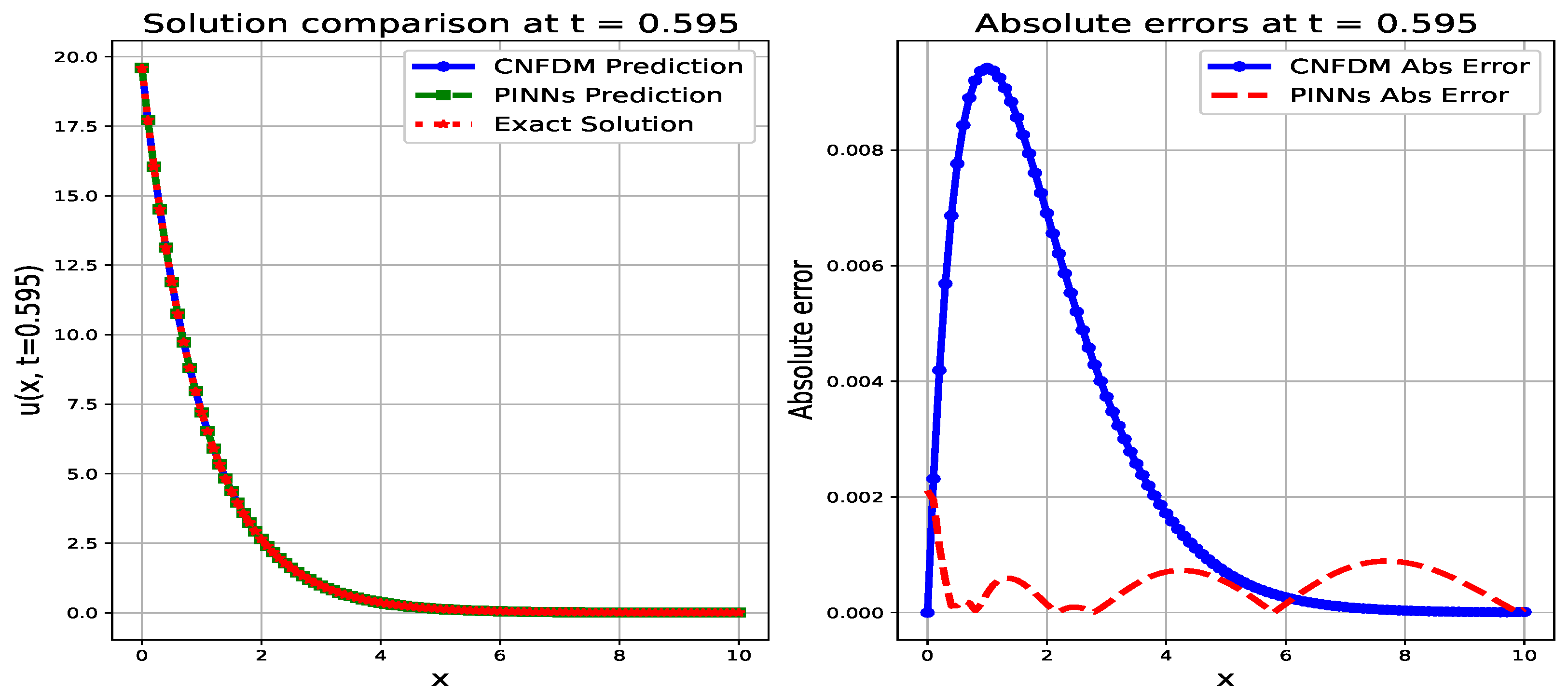
Figure 9 revealed that at $t=0.595$, the PINNs method was much more accurate than CNFDM. The biggest error for PINNs was only 0.000709, which is significantly smaller than CNFDM’s largest error of 0.009419. However, CNFDM maintains perfect accuracy at the boundary, with an error of 0.000000 at $x=0.0$, while PINNs have a small error of 0.000257 at that point. This divergence is visible in the error distribution plot, where the CNFDM error is highly concentrated into a single, very large peak near the boundary, while the PINNs absolute error, despite its lower peak magnitude, is highly non-uniform and oscillatory across the spatial domain.

5.8. Results for the CNFDM, PINNs and Exact Solutions at t = 0.680

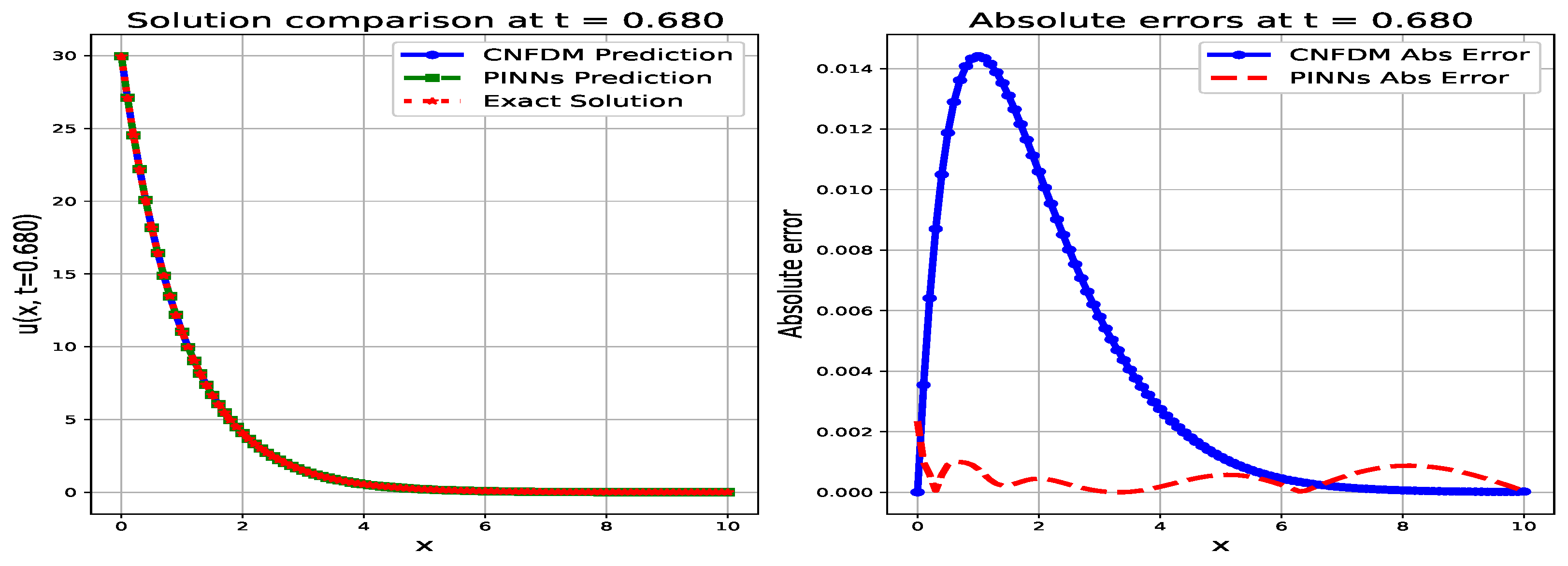
PINNs have a much lower maximum absolute error at $t=0.680$, peaking at 0.000467 (at $x=6.0$), as shown in Figure 10. This is in stark contrast to the CNFDM, whose maximum error has increased to a discernible 0.014411 at ($x=1.0$). Nevertheless, an examination of the boundary condition shows that PINNs experiences a tiny inaccuracy of 0.000202 at $x=0.0$, but CNFDM retains perfect precision with an error of 0.000000. The variation in spatial consistency is further made clear by an absolute error graphic. The absolute error of CNFDM is condensed into a single, enormous spike near the border, demonstrating how highly localised its errors are. The PINNs error, on the other hand, is not spatially uniform despite having a lower peak height; it is still oscillatory and dispersed over the domain, suggesting a less consistent performance over the whole solution space.

5.9. Results for the CNFDM, PINNs and Exact Solutions at t = 0.765

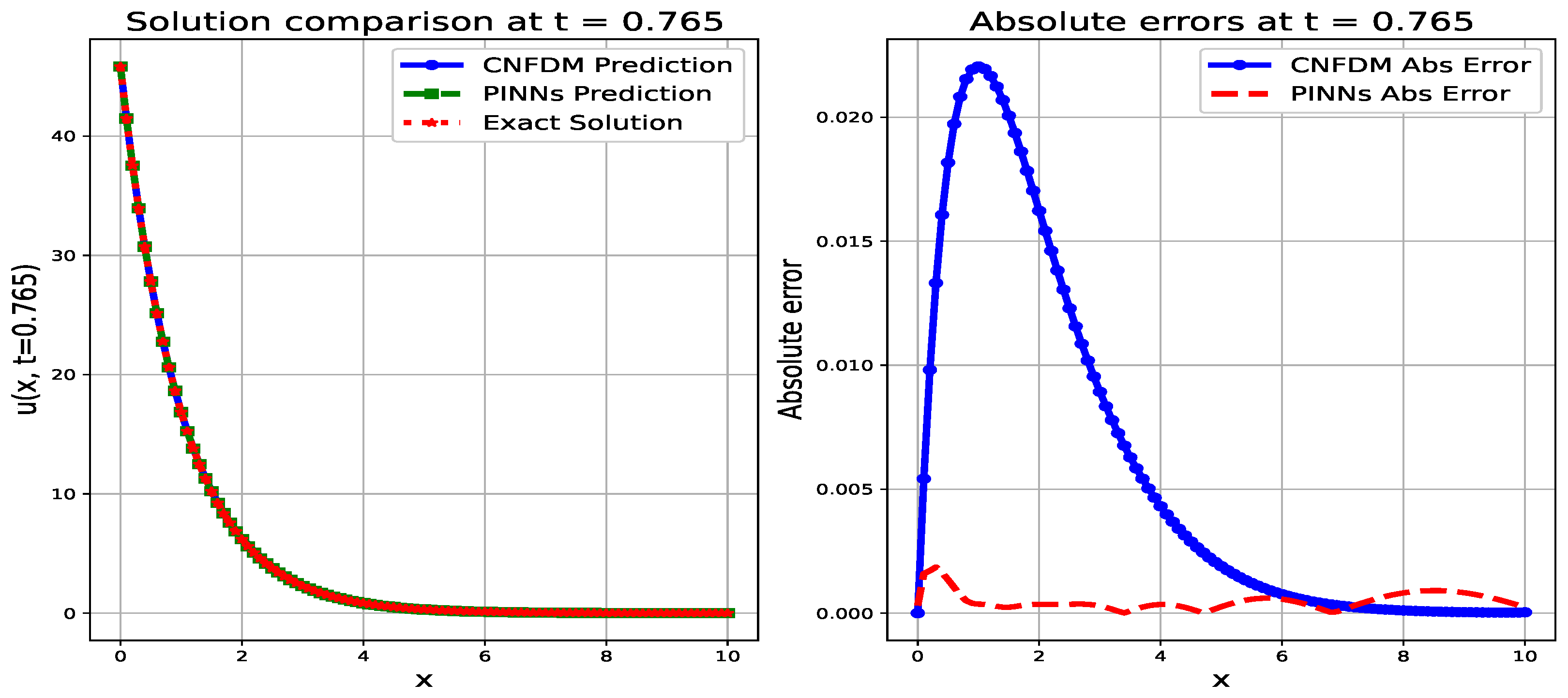
The continuous divergence in solution features between the two approaches is confirmed by the comparison analysis at t = 0.765 in Figure 11. The PINNs solution performs significantly better in terms of maximum absolute accuracy, registering a peak error of 0.000341 (at x = 0.0), orders of magnitude smaller than the CNFDM maximum error, which has sharply grown to 0.022044 (at x = 1.0). Nevertheless, at the x = 0.0 boundary, the CNFDM solution retains perfect precision with an error of 0.000000, while PINNs exhibits its maximum error at this location. While the PINNs error is less but still oscillatory and erratic throughout the solution domain, the CNFDM method’s spatial instability is highlighted in the error plot, where the error is concentrated into a single massive peak.

5.10. Results for the CNFDM, PINNs and Exact Solutions at t = 0.85

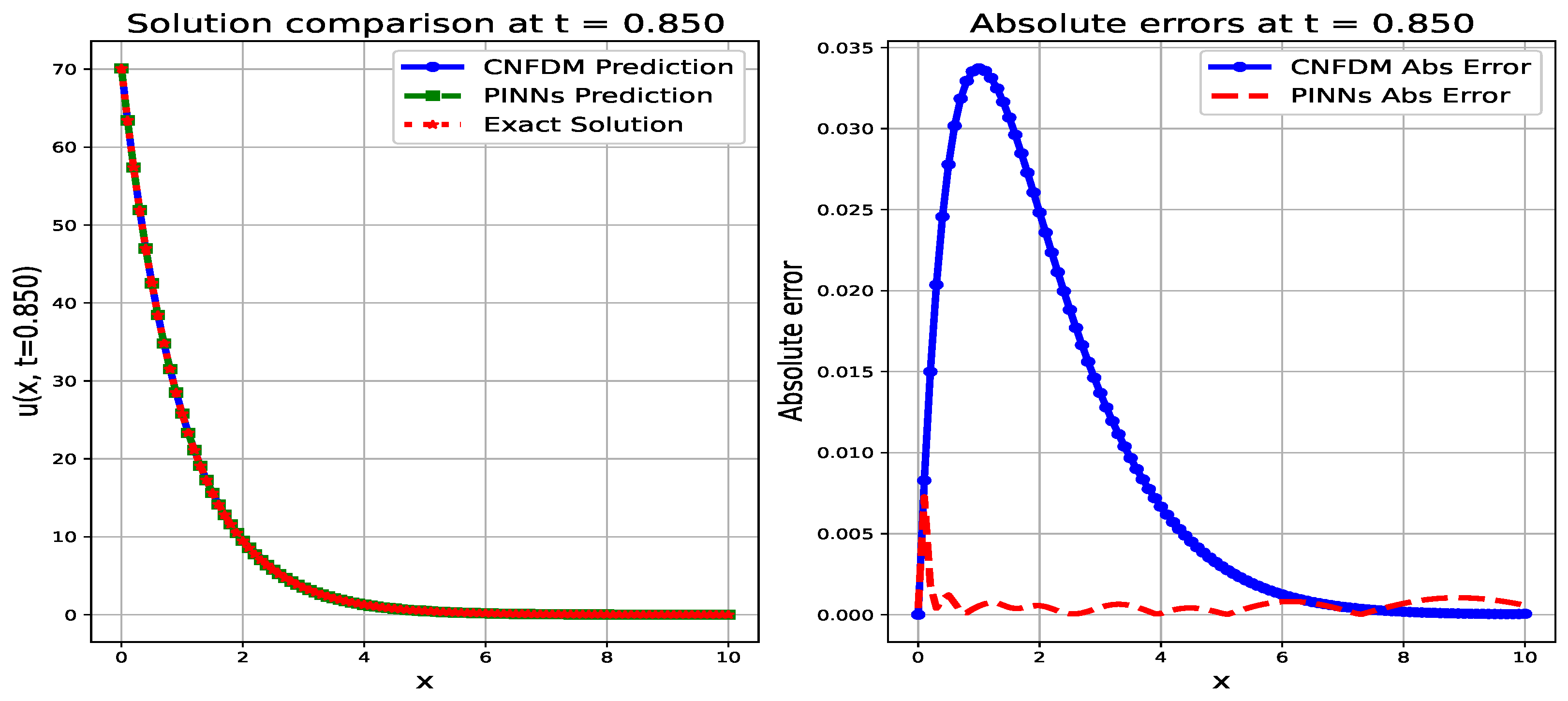
The PINNs solution has a considerable advantage in terms of maximum absolute accuracy at this later time step, as shown by the comparison study at $t=0.850$ in Figure 12. The greatest error of the PINNs solution was 0.006947 (at $x=0.0$), significantly less than the maximum error of the CNFDM solution, which peaked at 0.033719 (at $x=1.0$). On the other hand, CNFDM outperformed PINNs only at the $x=0.0$ boundary, where it maintained flawless precision with an error of 0.000000. The error distribution plot makes it evident that the PINNs absolute error, despite having a large peak at the boundary, typically maintains a lower and more oscillatory profile throughout the remainder of the spatial domain, while the CNFDM error is highly concentrated into one massive, spatially localized peak.

5.11. Results for the CNFDM, PINNs and Exact Solutions at x = 0.0

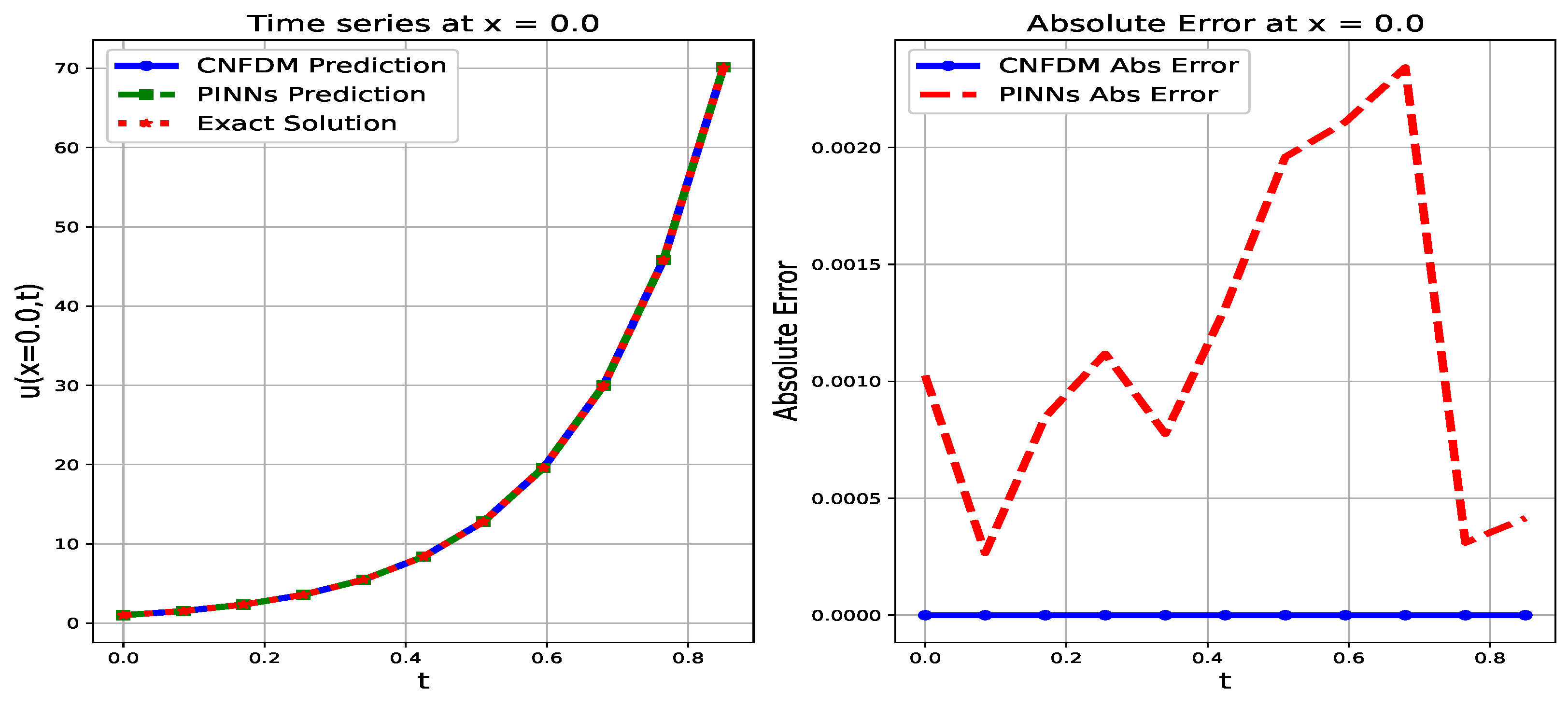
The results in Figure 13 show that the CNFDM method demonstrates perfect accuracy, consistency, and reliability since its values match the exact solution at all time steps with zero error, indicating a highly stable and precise numerical scheme. In contrast, the PINNs solution also closely follows the exact values with very small errors ranging mostly between ${10}^{-3}$ and ${10}^{-4}$, showing strong overall accuracy but with slight fluctuations over time, which reflects minor inconsistencies and a sensitivity to changes in the solution behavior as time progresses. The PINNs error does not remain constant, reaching its lowest point around $t=0.510$ and then increasing noticeably at $t=0.850$, which implies that although the neural network still performs reliably, its precision slightly decreases as the solution becomes more steep or complex. Overall, both methods perform well, but CNFDM clearly exhibits superior consistency and reliability, while PINNs maintain high accuracy with minor variations in performance over time.

5.12. Results for the CNFDM, PINNs and Exact Solutions at x = 1.0

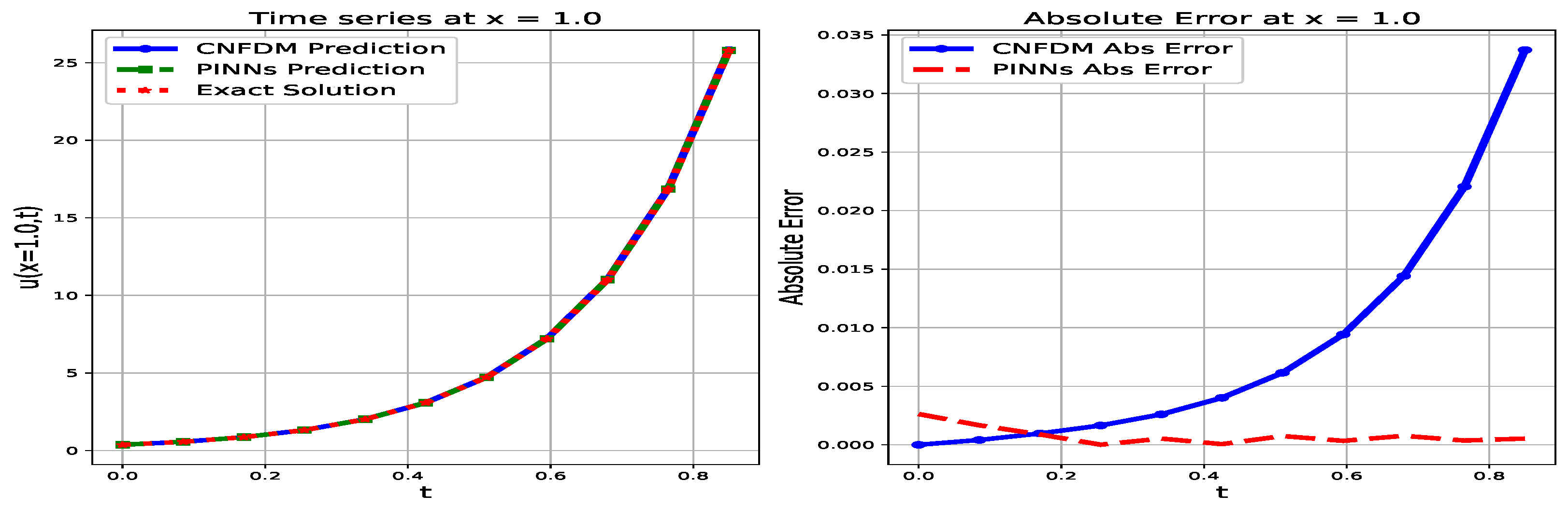
The results in Figure 14 show that at the initial time, CNFDM exactly matches the exact solution with zero error, while PINNs gives 0.369047 with an error of 0.001168. As time progresses, CNFDM begins to deviate gradually from the exact values, producing errors such as 0.000415 at $t=0.085$, and reaching 0.006153 at $t=0.510$. Eventually, the CNFDM error rises to 0.022044 at $t=0.765$ and 0.033719 at $t=0.850$, showing a steady growth in inaccuracy as the solution increases in magnitude. In contrast, the PINNs solution remains remarkably close to the exact solution across all time steps, producing small and stable errors such as 0.000290 at $t=0.085$, 0.000099 at $t=0.510$, and reaching its lowest error of 0.000012 at $t=0.765$. Even at the final time $t=0.850$, PINNs maintains a very small error of 0.000124. These trends indicate that while CNFDM gradually loses accuracy over time, PINNs maintains high fidelity to the exact solution, showing superior consistency, precision, and stability across the time domain.

5.13. Results for the CNFDM, PINNs and Exact Solutions at x = 2.0

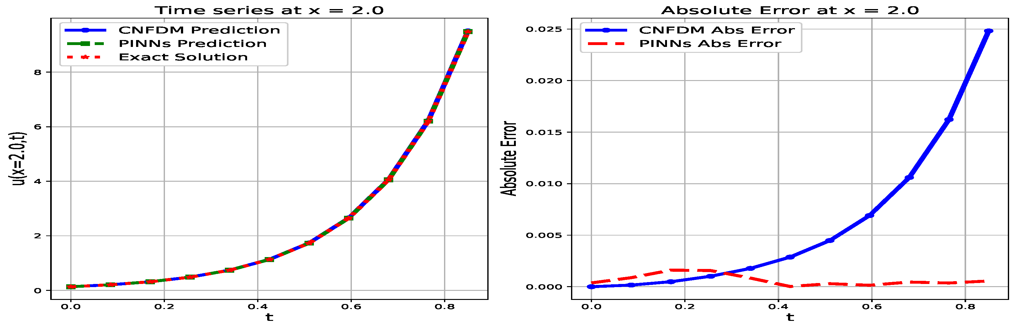
The comparison of CNFDM and PINNs solutions against the exact Solution at $x=2.0$, as illustrated in Figure 15, confirms that both numerical methods achieve a high level of accuracy, with their time series predictions closely following the steep growth of the exact solution curve. However, the analysis of the Absolute Error Plot reveals a dramatic divergence in their consistency and reliability. The CNFDM absolute error exhibits poor long-term consistency; it starts at zero (at $t=0.0$) and shows a clear, rapidly increasing trend over time, ultimately reaching its peak error of $0.024822$ at the end of the interval ($t=0.850$). This escalating error indicates a significant deterioration in the reliability of CNFDM as the simulation progresses. Consequently, while CNFDM initially has smaller errors, PINNs demonstrates vastly superior long-term reliability and consistency across the full time series, successfully containing its error to a small, nearly constant magnitude, unlike the continuously increasing error of CNFDM.

5.14. Results for the CNFDM, PINNs and Exact Solutions at x = 3.0

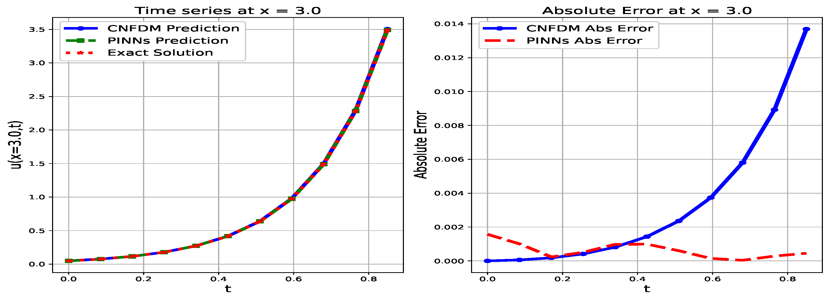
Figure 16 demonstrates the excellent level of accuracy for both numerical techniques. However, there are noticeable differences in their consistency and dependability when comparing the Absolute Error Plot. The CNFDM absolute error has poor long-term consistency, reaching its greatest value of $0.013688$ at $t=0.850$. It begins close to zero but shows a notable and fast increasing tendency over time. This increasing error distribution indicates that as the simulation runs longer and the solution magnitude increases, CNFDM’s reliability declines dramatically. In contrast, the PINNs absolute error shows a relatively stable and bounded distribution that remains very small across the domain, fluctuating between a high of $0.000875$ at $t=0.170$ and a low of $0.000039$ at $t=0.680$. For the latter half of the time series ($t>0.4$), the PINNs error is consistently and significantly lower than the CNFDM error. Overall, PINNs shows better consistency and longer-term reliability over the observed interval, successfully retaining very tiny errors even as the solution increases steeper, even though both approaches are quite precise.

5.15. Results for the CNFDM, PINNs and Exact Solutions at x = 4.0

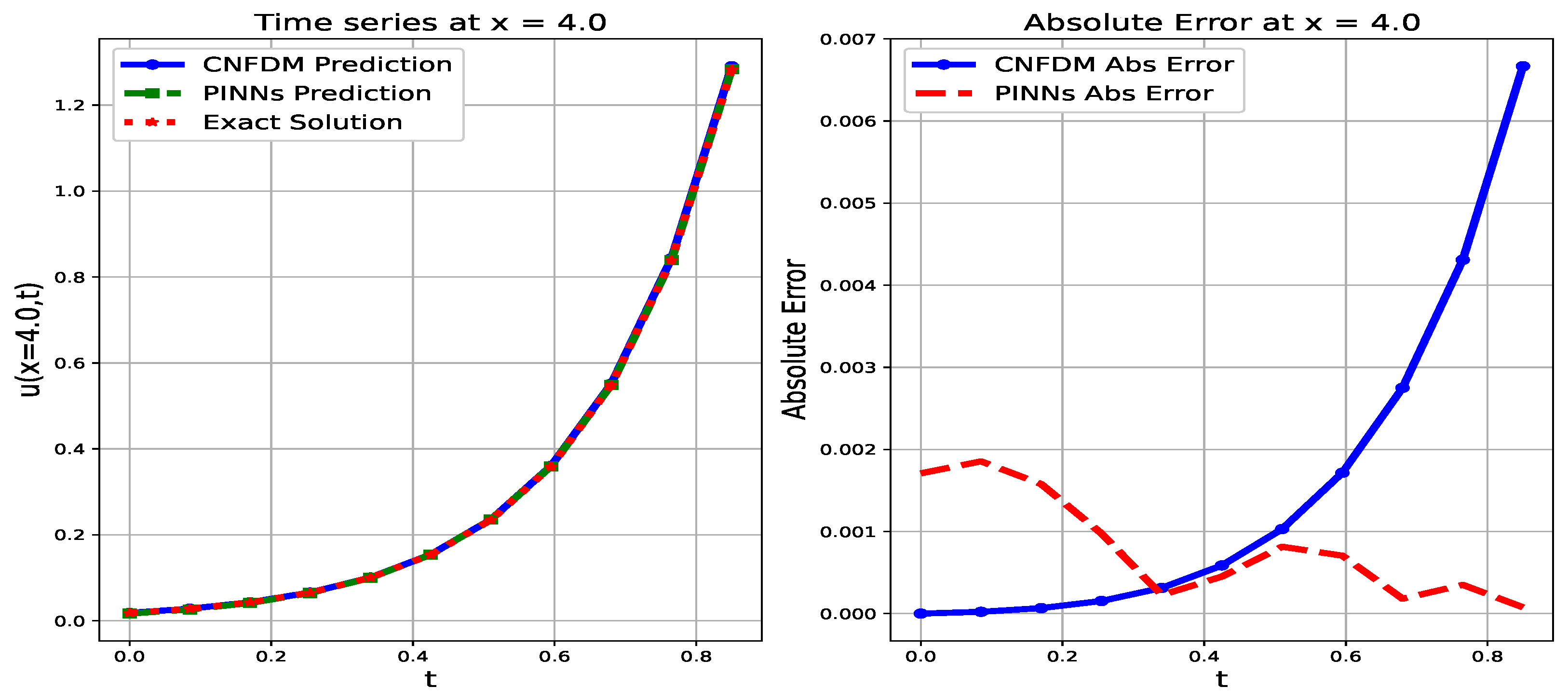
When comparing the numerical solutions to the exact solution at $x=4.0$ in Figure 17, both the CNFDM and PINNs approaches show a high degree of accuracy, as demonstrated by their close agreement in the time series plot. However, significant variations in their consistency and dependability are shown upon closer examination of the Absolute Error Plot. Long-term consistency is lacking in the CNFDM approach because its absolute error, which begins at zero, increases quickly and dramatically with time, peaking at $0.006668$ at $t=0.850$. As the simulation period increases and the values of the solution rise, this increasing trend in the error suggests a dramatic drop in the reliability of CNFDM. In contrast, the PINNs absolute error maintains a notably stable and bounded distribution of minimal values across the entire domain. While it has a slight peak of $0.000736$ at $t=0.425$, the PINNs error is consistently and substantially lower than the CNFDM error for the second half of the time series ($t>0.510$). Therefore, although both techniques are highly precise, PINNs prove to be more reliable and consistent over the longer term, successfully keeping the errors extremely small even as the solution becomes increasingly steep (see Figure 17).

5.16. Results for the CNFDM, PINNs and Exact Solutions at x = 5.0

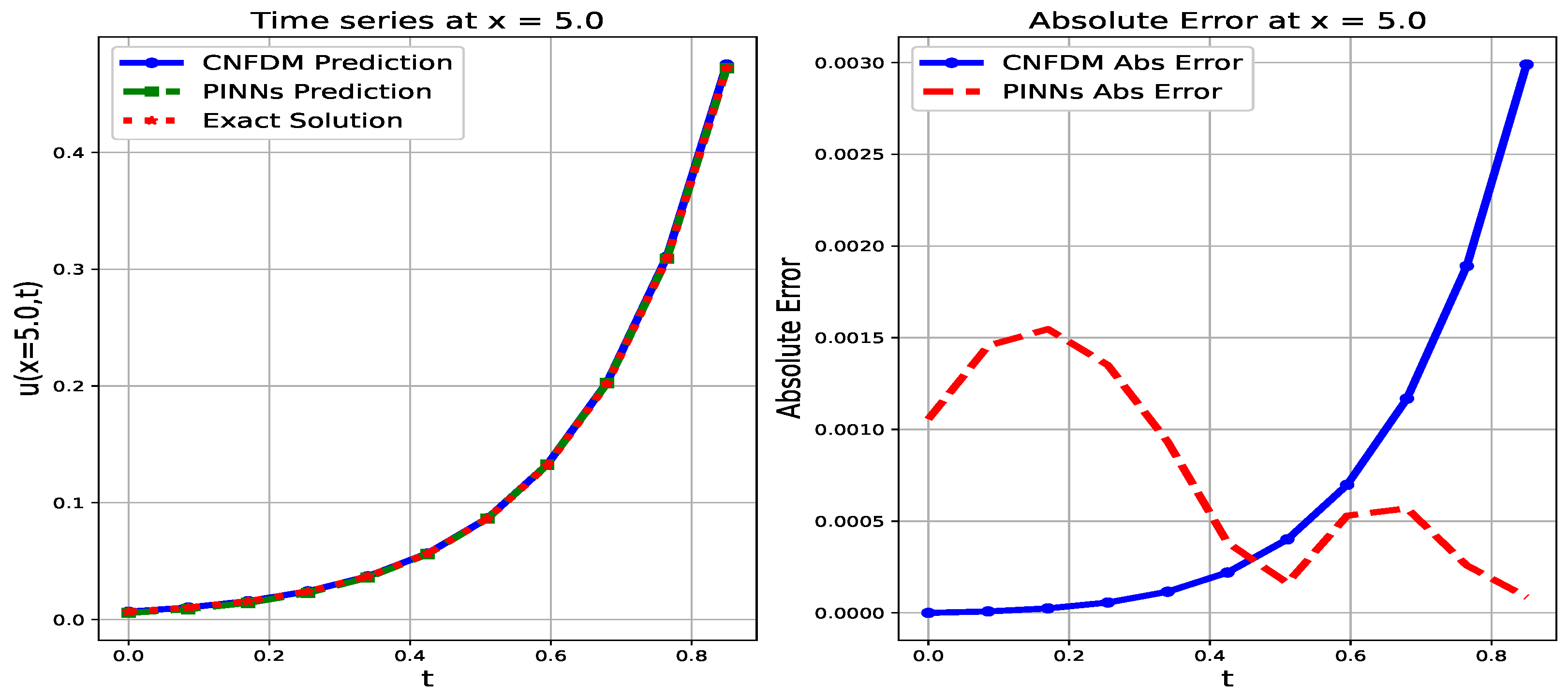
A high level of accuracy for both numerical methods is confirmed by the results shown in Figure 18, which compare the CNFDM and PINNs solutions against the exact solution at $x=5.0$. This is because their predictions closely match the exact solution over the entire time series. However, there are clear trends in their consistency and dependability when the Absolute Error Plot is analyzed. The CNFDM absolute error demonstrates poor long-term consistency; it starts at zero and shows a clear, rapid increasing trend over time, peaking at $0.002989$ at $t=0.850$. This escalating error suggests a significant decrease in CNFDM’s reliability as the simulation time extends and the solution magnitude increases. In contrast, the PINNs absolute error exhibits a more stable and bounded distribution of small values across the domain, fluctuating between a low of $0.000063$ at $t=0.255$ and a high of $0.000753$ at $t=0.510$. For the final two time points ($t=0.765$ and $t=0.850$), the PINNs error is substantially lower than the CNFDM error, showing values of $0.000056$ and $0.000115$, respectively. Overall, while both methods are highly accurate, PINNs demonstrates superior long-term reliability and consistency, successfully maintaining extremely small error values even as the solution becomes steeper at the end of the observed interval.

5.17. Results for the CNFDM, PINNs and Exact Solutions at x = 6.0

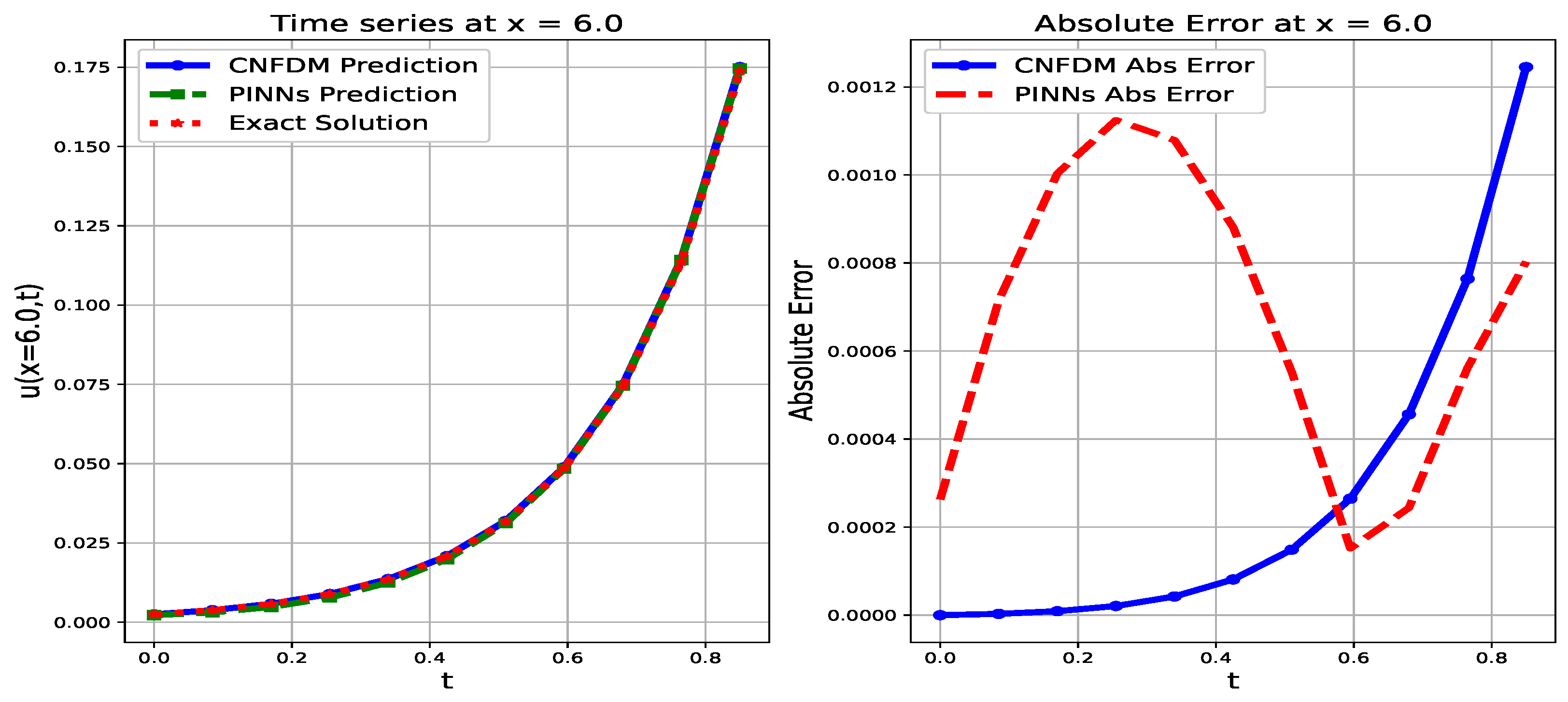
Both approaches show a high degree of accuracy, with their time series forecasts nearly matching the exact solution curve, as seen by the results from Figure 19, which compare the CNFDM and PINNs solutions against the exact solution at $x=6.0$. When looking at the Absolute Error Plot, however, their consistency and reliability are different. The CNFDM absolute error exhibits poor long-term stability; it begins close to zero but exhibits a distinct, sharply rising trend with time, peaking at $0.001245$ at $t=0.850$. As the simulation period increases and the solution magnitude grows, this increasing inaccuracy indicates a sharp decline in CNFDM’s reliability. In contrast, the PINNs absolute error displays a more stable and bounded distribution of small values that fluctuates across the domain. The PINNs error begins around $0.000339$, peaks around $t=0.170$ at $0.000425$, drops to its lowest point of $0.000052$ at $t=0.425$, then peaks again at $t=0.680$ at $0.000467$, before falling slightly to $0.000296$ at $t=0.850$. Notably, the PINNs error is substantially lower than the CNFDM error at the end of the interval. Overall, while both methods are highly accurate, PINNs demonstrates superior long-term reliability and consistency, successfully maintaining very small, bounded error values even as the solution becomes steeper.

5.18. Results for the CNFDM, PINNs and Exact Solutions at x = 7.0

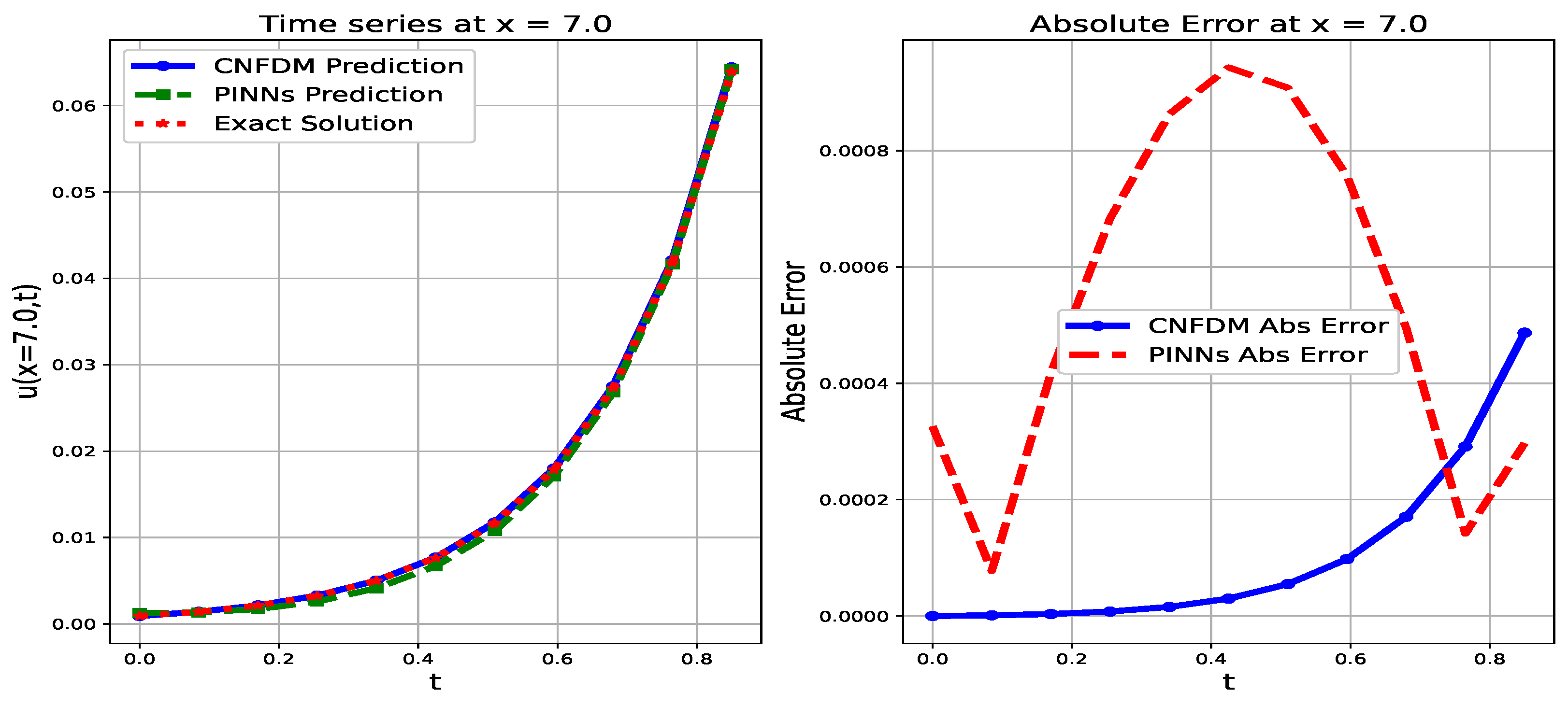
Both numerical methods are quite precise, closely following the exact solution curve, as shown by the comparison of CNFDM and PINNs solutions against the exact solution at $x=7.0$, as presented in Figure 20. When examining the Absolute Error Plot, however, their consistency and reliability differ. The CNFDM absolute error demonstrates poor long-term consistency; it starts at zero but rises rapidly and gradually over time, peaking at $0.000487$ at $t=0.850$. This growing inaccuracy indicates a sharp decline in the reliability of CNFDM as the simulation lengthens and the solution magnitude increases. On the other hand, at $t=0.255$, the PINNs absolute error peaks at $0.000501$ after initial fluctuations. For the remainder of the interval, however, it quickly stabilises into a more stable and bounded distribution, reaching a low of $0.000062$ at $t=0.680$. Remarkably, the PINNs error is substantially lower than the CNFDM error in the critical late phases ($t\ge 0.680$). Although both approaches are accurate, PINNs shows superior long-term reliability and consistency compared to CNFDM’s steadily rising error, effectively preserving extremely small, bounded error values in the latter half of the time series.

5.19. Results for the CNFDM, PINNs and Exact Solutions at x = 8.0

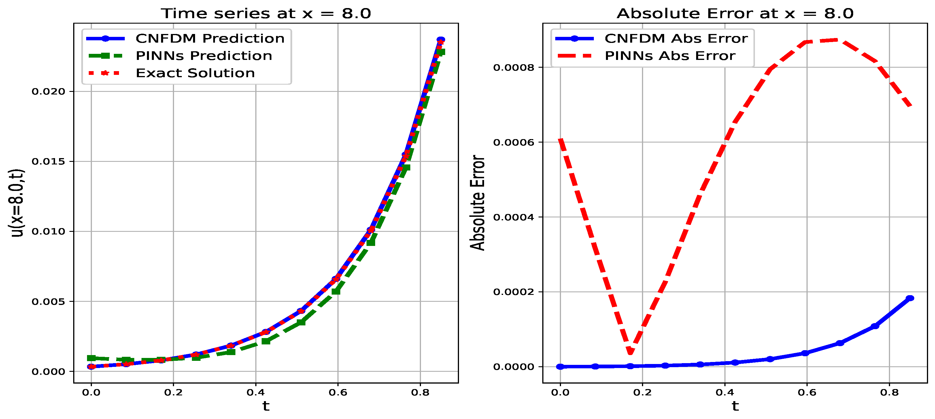
Both numerical methods are extremely accurate, with their predictions closely following the exact solution curve, as shown by the comparison of CNFDM and PINNs solutions against the exact solution at $x=8.0$, as presented in Figure 21. However, when examining the absolute error map, their consistency and reliability show radically distinct tendencies. The PINNs absolute error follows a non-monotonic, bell-shaped distribution that is stable and bounded, starting at $0.000161$, rapidly increasing to a maximum error of $0.000475$ at $t=0.340$, and then continuously decreasing to a minimum of $0.000051$ at $t=0.850$. This bounded behavior demonstrates the high reliability of the PINNs method over the entire interval. The CNFDM absolute error, on the other hand, exhibits poor long-term consistency; it begins close to zero (at $t=0.0$) and shows a distinct, rapidly rising trend over time. The error increases steadily, reaching a peak of $0.000183$ at the conclusion of the observation time frame ($t=0.850$) and eventually surpassing the PINNs error around $t=0.765$. Therefore, despite having slightly higher errors in the early-to-mid stages, the PINNs approach ultimately provides superior long-term reliability and consistency due to its stable, converging error distribution, whereas the continuously growing error of CNFDM suggests declining reliability as the solution steepens.

5.20. Results for the CNFDM, PINNs and Exact Solutions at x = 9.0

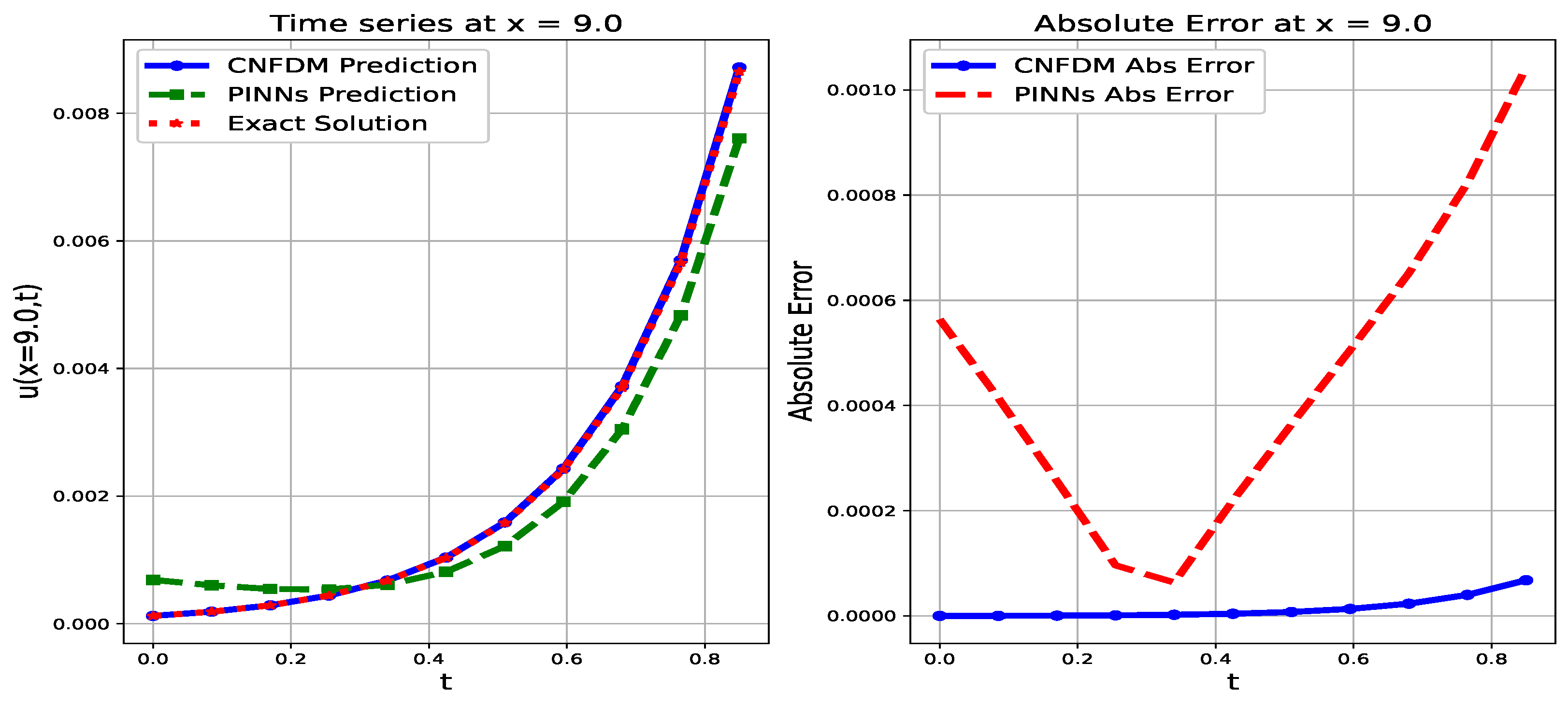
Both numerical methods are very accurate, with their predictions closely following the exact solution curve, as shown by the comparison of CNFDM and PINNs solutions against the exact solution at $x=9.0$, as presented in Figure 22. However, when examining the absolute error, their consistency and reliability show radically different patterns. The CNFDM absolute error demonstrates a consistently low magnitude of error throughout the simulation, starting at zero and increasing very slowly to a peak of only $0.000068$ at $t=0.850$. Although this trend is increasing, the extremely small values indicate a very high degree of accuracy and reliability across the entire range. Conversely, the PINNs absolute error follows a bell-shaped, but bounded, distribution that is substantially larger than the CNFDM error, peaking at $0.000361$ at $t=0.595$ before decreasing to $0.000223$ at $t=0.850$. Therefore, while the PINNs error shows better consistency in its bounded distribution, the CNFDM method demonstrates significantly superior overall accuracy and reliability at this location due to its much lower error magnitude across all time steps.

5.21. Results for the CNFDM, PINNs and Exact Solutions at x = 10.0

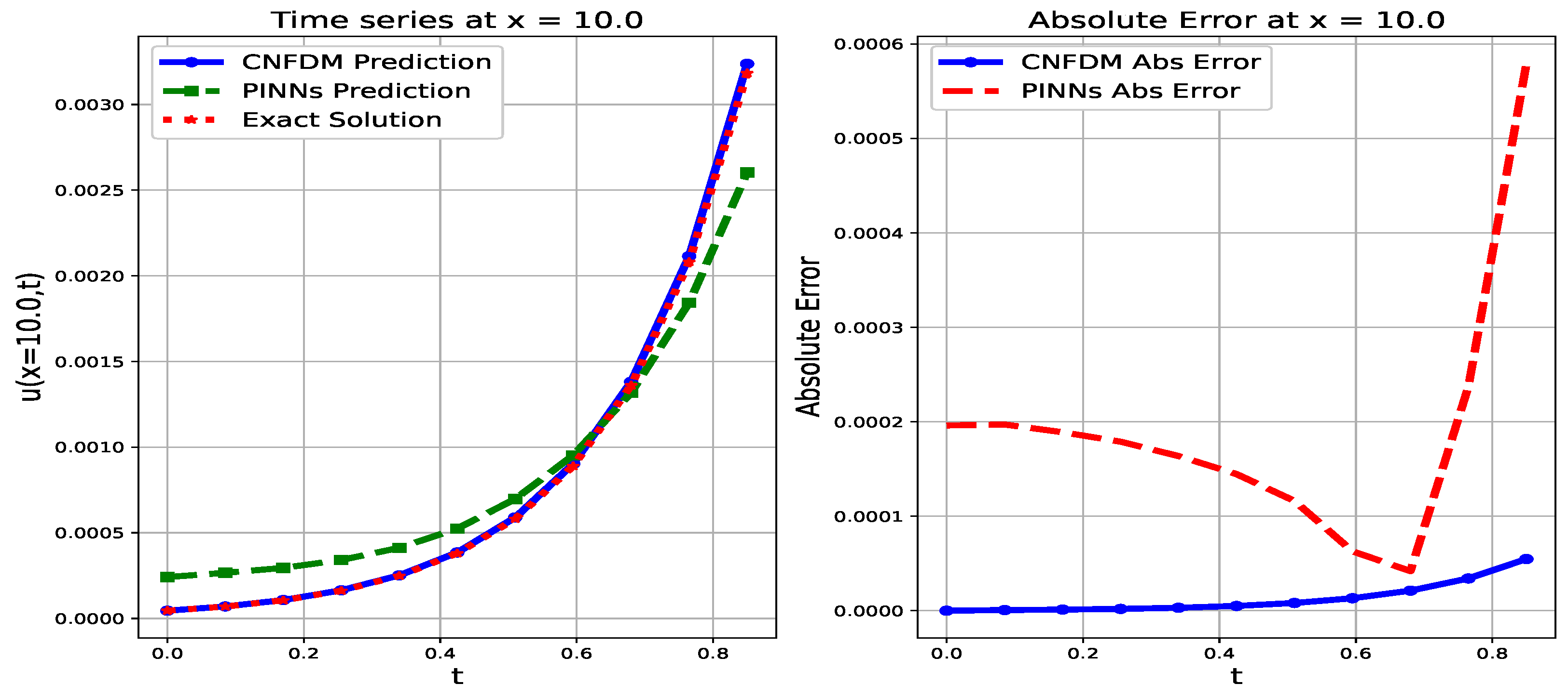
The comparison of CNFDM and PINNs solutions against the exact solution at $x=10.0$, as shown in Figure 23, confirms that both numerical techniques are highly accurate, with their predictions closely tracking the exact solution curve over the observed interval. However, their consistency and reliability show significantly different trends when analyzing the Absolute Error Plot. The CNFDM absolute error demonstrates superior overall accuracy and excellent long-term consistency; it starts at zero ($0.000000$ at $t=0.0$) and, although it exhibits a continuously increasing trend, it remains very small, peaking at only $0.000055$ at $t=0.850$. This consistently low error indicates a very high degree of reliability across the entire range. In sharp contrast, the PINNs absolute error follows a rapidly increasing trend across the domain, starting at $0.000048$ at $t=0.0$ and reaching a maximum error of $0.000310$ at $t=0.850$. Notably, the PINNs error is substantially higher than the CNFDM error for nearly the entire time series (except around $t=0.085$). Because of its much lower error magnitude over all time steps, the CNFDM technique exhibits far higher accuracy and superior long-term reliability at this location, even though both methods are accurate.

6. Conclusions

• This research successfully executed a PINNs framework and the CNFDM to approximate the solution of the governing ADR equation.
• The comparison between CNFDM and PINNs in solving the ADR equation shows that both methods reach a high degree of accuracy; however, their performance traits vary notably in different time frames and spatial contexts.
• The CNFDM consistently demonstrates flawless accuracy at the boundary x = 0.0 throughout all time levels and shows outstanding performance during the initial time phases, especially when the solution profile is smooth and has a gentle slope. Moreover, CNFDM provides an outstanding benefit in computation, finishing the simulation in only one second, unlike the considerably greater computational expense required by PINNs.
• The CNFDM error progressively increases across the inner region as time goes on and the solution becomes sharper, especially at later time points, indicating a gradual decrease in both accuracy and spatial consistency. PINNs, on the other hand, show low, constrained, and reliable error levels at the majority of interior spatial locations, even over time and under difficult solution conditions. This highlights their exceptional long-term dependability, resilience to error buildup, and ability to adjust to intricate spatiotemporal dynamics.
• These findings recommend the use of CNFDM for problems that call for quick computations, quick evaluations, and accurate boundary control, particularly where the boundaries are the primary emphasis or the solution is smooth. However, situations with steep gradients, long-term simulations, and accuracy in the interior domain where stability and consistency over time are essential and better suited for PINNs.
• Future studies may look at hybrid models that combine the speed and boundary precision of CNFDM with the long-term accuracy and robustness of PINNs. Furthermore, using transfer learning, domain decomposition, or adaptive loss weighting to improve PINNs could lower computational costs without sacrificing accuracy. To improve the evaluation of physical interpretability, efficiency, and scalability, more research could extend the use of PINNs to higher-dimensional ADR equations and parameter identification.

References

1. Rubio, A.; Zalts, A.; El Hasi, C. Numerical solution of the advection–reaction–diffusion equation at different scales. Environ. Model. Softw. 2008, 23, 90–95. [Google Scholar] [CrossRef] [Scilit]
2. Guenneau, S.; Petiteau, D.; Zerrad, M.; Amra, C.; Puvirajesinghe, T. Transformed Fourier and Fick equations for the control of heat and mass diffusion. AIP Adv. 2015, 5, 053404. [Google Scholar] [CrossRef] [Scilit]
3. Aris, R. On the dispersion of a solute in a fluid flowing through a tube. Proc. R. Soc. Lond. Ser. A Math. Phys. Sci. 1956, 235, 67–77. [Google Scholar] [CrossRef] [Scilit]
4. Taylor, G. Dispersion of soluble matter in solvent flowing slowly through a tube. Proc. R. Soc. Lond. Ser. A Math. Phys. Sci. 1953, 219, 186–203. [Google Scholar] [CrossRef] [Scilit]
5. Crank, J. The Mathematics of Diffusion; Oxford University Press: Oxford, UK, 1979. [Google Scholar]
6. El Arabi, I.; Chafi, A.; Alami, S. Numerical simulation of the advection-diffusion-reaction equation using finite difference and operator splitting methods: Application on the 1D transport problem of contaminant in saturated porous media. E3S Web Conf. 2022, 351, 01003. [Google Scholar] [CrossRef] [Scilit]
7. Jerves, A. An analysis of classical techniques for consistent stabilisation of the advection–diffusion–reaction equation finite element solution. Int. J. Comput. Fluid Dyn. 2020, 34, 315–332. [Google Scholar] [CrossRef] [Scilit]
8. Rawat, R.; Pandey, C.; Kumar, B.; Thije Boonkkamp, J. A Finite Volume Complete Flux Scheme for Time Fractional ADR Equation. 2023. Available online: https://istam.iitkgp.ac.in/resources/2023/proceedings/Abstract/PA0271.pdf (accessed on 6 September 2023).
9. Raissi, M.; Perdikaris, P.; Karniadakis, G. Physics-informed neural networks: A deep learning framework for solving forward and inverse problems involving nonlinear partial differential equations. J. Comput. Phys. 2019, 378, 686–707. [Google Scholar] [CrossRef] [Scilit]
10. Karniadakis, G.; Kevrekidis, I.; Lu, L.; Perdikaris, P.; Wang, S.; Yang, L. Physics-informed machine learning. Nat. Rev. Phys. 2021, 3, 422–440. [Google Scholar] [CrossRef] [Scilit]
11. Cuomo, S.; Di Cola, V.; Giampaolo, F.; Rozza, G.; Raissi, M.; Piccialli, F. Scientific machine learning through physics–informed neural networks: Where we are and what’s next. J. Sci. Comput. 2022, 92, 88. [Google Scholar] [CrossRef] [Scilit]
12. Dwivedi, V.; Srinivasan, B. Physics Informed Extreme Learning Machine (PIELM)—A rapid method for the numerical solution of partial differential equations. arXiv 2019, arXiv:1907.03507. [Google Scholar] [CrossRef] [Scilit]
13. Liu, X.; Yao, W.; Peng, W.; Zhou, W. Bayesian Physics-Informed Extreme Learning Machine for Forward and Inverse PDE Problems with Noisy Data. Neurocomputing 2023, 549, 126425. [Google Scholar] [CrossRef] [Scilit]
14. Alamdari, B.; Tang, Y.; Erricolo, D.; Sneed, L. A Comprehensive Review of GPR Data Analysis for Bridge Deck Evaluation: From Conventional Methods to Emerging Artificial Intelligence Approaches. J. Nondestruct. Eval. 2025, 45, 15. [Google Scholar] [CrossRef] [Scilit]
15. Ren, Y.; Zhang, J.; Xia, Y.; Wang, R.; Xie, F.; Guan, J.; Zhang, H.; Zhou, S. Regression-based conditional independence test with adaptive kernels. Artif. Intell. 2025, 347, 104391. Available online: https://www.sciencedirect.com/science/article/pii/S0004370225001109 (accessed on 1 July 2025). [CrossRef] [Scilit]
16. Qian, S.; Chen, Y.; Wang, W.; Zhang, G.; Li, L.; Hao, Z.; Wang, Y. Physics-guided deep neural networks for bathymetric mapping using Sentinel-2 multi-spectral imagery. Front. Mar. Sci. 2025, 12, 1636124. Available online: https://www.frontiersin.org/journals/marine-science/articles/10.3389/fmars.2025.1636124 (accessed on 26 August 2025). [CrossRef] [Scilit]
17. Kamyab, S.; Azimifar, Z.; Sabzi, R.; Fieguth, P. Deep learning methods for inverse problems. PeerJ Comput. Sci. 2022, 8, e951. [Google Scholar] [CrossRef] [Scilit] [PubMed]
18. Chen-Charpentier, B.; Kojouharov, H. An unconditionally positivity preserving scheme for advection–diffusion reaction equations. Math. Comput. Model. 2013, 57, 2177–2185. [Google Scholar] [CrossRef] [Scilit]
19. Kopp, R. Pontryagin maximum principle. Math. Sci. Eng. 1962, 5, 255–279. [Google Scholar]
20. Wu, T.; Xu, X. Semi-global stabilization of parabolic PDE–ODE systems with input delay and saturation. Int. J. Syst. Sci. 2025, 1–19. [Google Scholar] [CrossRef] [Scilit]
21. Xu, X.; Li, B. PDE-based observation and predictor-based control for linear systems with distributed infinite input and output delays. Automatica 2024, 170, 111845. Available online: https://www.sciencedirect.com/science/article/pii/S000510982400339X (accessed on 26 August 2025). [CrossRef] [Scilit]
22. Crank, J.; Nicolson, P. A practical method for numerical evaluation of solutions of partial differential equations of the heat-conduction type. Math. Proc. Camb. Philos. Soc. 1947, 43, 50–67. [Google Scholar] [CrossRef] [Scilit]
Figure 1. Schematic representation depicting the architecture of Physics-Informed Neural Networks (PINNs) utilized for the Advection–Diffusion–Reaction equation.
Mathematics 14 01194 g001
Figure 2. Number of epochs vs. PINNs training loss.
Mathematics 14 01194 g002
Figure 3. Comparison of numerical solutions from CNFDM and PINNs vs. the exact solution at t = 0.085 .
Mathematics 14 01194 g003
Figure 4. Comparison of numerical solutions from CNFDM and PINNs vs. the exact solution at t = 0.170 .
Mathematics 14 01194 g004
Figure 5. Comparison of numerical solutions from CNFDM and PINNs vs. the exact solution at t = 0.255 .
Mathematics 14 01194 g005
Figure 6. Comparison of numerical solutions from CNFDM and PINNs vs. the exact solution at t = 0.340 .
Mathematics 14 01194 g006
Figure 7. Comparison of numerical solutions from CNFDM and PINNs vs. the exact solution at t = 0.425 .
Mathematics 14 01194 g007
Figure 8. Comparison of numerical solutions from CNFDM and PINNs vs. the exact solution at t = 0.510 .
Mathematics 14 01194 g008
Figure 9. Comparison of numerical solutions from CNFDM and PINNs vs. the exact solution at t = 0.595 .
Mathematics 14 01194 g009
Figure 10. Comparison of numerical solutions from CNFDM and PINNs vs. the exact solution at t = 0.680 .
Mathematics 14 01194 g010
Figure 11. Comparison of numerical solutions from CNFDM and PINNs vs. the exact solution at t = 0.765 .
Mathematics 14 01194 g011
Figure 12. Comparison of numerical solutions from CNFDM and PINNs vs. the exact solution at t = 0.850 .
Mathematics 14 01194 g012
Figure 13. Comparison of numerical solutions from CNFDM and PINNs vs. the exact solution at x = 0 .
Mathematics 14 01194 g013
Figure 14. Comparison of numerical solutions from CNFDM and PINNs vs. the exact solution at x = 1 .
Mathematics 14 01194 g014
Figure 15. Comparison of numerical solutions from CNFDM and PINNs vs. the exact solution at x = 2 .
Mathematics 14 01194 g015
Figure 16. Comparison of numerical solutions from CNFDM and PINNs vs. the exact solution at x = 3 .
Mathematics 14 01194 g016
Figure 17. Comparison of numerical solutions from CNFDM and PINNs vs. the exact solution at x = 4 .
Mathematics 14 01194 g017
Figure 18. Comparison of numerical solutions from CNFDM and PINNs vs. the exact solution at x = 5 .
Mathematics 14 01194 g018
Figure 19. Comparison of numerical solutions from CNFDM and PINNs vs. the exact solution at x = 6 .
Mathematics 14 01194 g019
Figure 20. Comparison of numerical solutions from CNFDM and PINNs vs. the exact solution at x = 7 .
Mathematics 14 01194 g020
Figure 21. Comparison of numerical solutions from CNFDM and PINNs vs. the exact solution at x = 8 .
Mathematics 14 01194 g021
Figure 22. Comparison of numerical solutions from CNFDM and PINNs vs. the exact solution at x = 9 .
Mathematics 14 01194 g022
Figure 23. Comparison of numerical solutions from CNFDM and PINNs vs. the exact solution at x = 10 .
Mathematics 14 01194 g023