New Relations on the Critical Line: Riemann Zeta Zeros, Divergent Series, and Infinite Numbers

Abstract

In this work, a formal asymptotic framework based on infinite number expressions is employed to investigate structural relations associated with the Dirichlet representation of the Riemann zeta function. Within this framework, infinite number objects are interpreted through asymptotic representatives and serve as symbolic encodings of asymptotic behavior in the regime x → ∞. A divergent real series is constructed from the sum of entries of an n × n matrix in the asymptotic limit n → ∞ and analyzed in relation to the squared modulus of a Dirichlet-type series. When the common parameter coincides with the imaginary part of a nontrivial zero of the Riemann zeta function on the critical line, the framework yields a structured cancellation mechanism, leading to parameter-dependent decay or convergence toward the constant −γ/2. Additional formal asymptotic relations are derived linking nontrivial zeros, divergent expressions, and the Euler–Mascheroni constant. The theoretical analysis is accompanied by numerical computations in double-precision arithmetic, which serve as consistency checks of the predicted asymptotic behavior. The proposed approach provides a coherent representative asymptotic methodology for organizing and analyzing identities involving divergent expressions arising in analytic number theory. The resulting relations are interpreted within this representative framework and are intended as structural asymptotic identities rather than classical equalities of divergent series.

1. Introduction

Leonhard Euler first introduced and studied the zeta function ζ(s), initially defined for real arguments by the Dirichlet series

$$\zeta (s)={\displaystyle \sum _{n=1}^{\infty }\frac{1}{n^s}}$$

(1)

which converges for ℜ(s) > 1. In his seminal 1859 memoir [1], Bernhard Riemann extended Euler’s definition to a complex variable and established its analytic continuation. Riemann showed that ζ(s) admits a meromorphic continuation to the entire complex plane ℂ, with a single simple pole at s = 1.

Among the most important structural properties of the Riemann zeta function are those arising from its functional equation. In particular:

(i)

ζ(s) has no zeros for ℜ(s) > 1;

(ii)

The only pole occurs at s = 1, with residue value equal to 1;

(iii)

ζ(s) possesses trivial zeros at s = −2, −4, −6, …;

(iv)

The nontrivial zeros of ζ(s) lie within the critical strip 0 < ℜ(s) < 1 and are symmetric with respect to both the critical line ℜ(s) = 1/2 and the real axis.

Hardy’s theorem (1914) [2,3] established that infinitely many nontrivial zeros lie on the critical line. The study of the distribution and structural properties of these zeros remains central to analytic number theory.

The present work does not attempt to modify or reinterpret the classical analytic structure of the Riemann zeta function. Instead, it adopts a formal asymptotic framework—based on infinite number representations introduced in [4]—with the aim of deriving alternative identities involving divergent or asymptotic expressions associated with ζ(s). This perspective is complementary to, and not in conflict with, established analytic number theory. Throughout the paper, all identities are understood within the infinite number representative framework described in Section 2.

The mathematical formalization of infinity has a long and well-established history, beginning with the foundational work of Dedekind, Cantor, and Frege in the nineteenth century [5,6,7,8,9,10], and extending through Robinson’s development of Nonstandard Analysis [11,12,13,14], later refined and expanded by Keisler [15]. The framework employed here differs from classical nonstandard models; it operates instead as a formal asymptotic calculus in which expressions involving divergence are encoded and manipulated through infinite number representations defined via limiting procedures.

In [4], so-called infinite numbers were introduced as formal asymptotic constructs together with associated calculation rules. These works defined a class of asymptotic representations together with differentiation and integration procedures consistent with their formal structure. Within that setting, divergent or non-ordinary series may be expressed in normal form and analyzed through representative functions. Subsequent studies [16,17] extended this formalism to the analysis of the Riemann zeta function, including the introduction of rotational infinite number representations and the derivation of identities involving nontrivial zeros.

In particular, ref. [17] established relations connecting nontrivial zeros of ζ(s) with the Euler–Mascheroni constant γ, and provided asymptotic decompositions of certain divergent Dirichlet-type expressions when ℜ(s) = 1/2. These developments motivate the present investigation.

In this work, we further explore structural relations arising when series constructed from an n × n matrix (with n → ∞) are compared with expressions derived from the Dirichlet series representation of ζ(s) on the critical line. The analysis yields explicit identities linking matrix-defined sums, squared moduli of truncated Dirichlet expressions, and quantities involving nontrivial zeros. These results are derived entirely within the formal infinite number framework introduced in Section 2.

The contribution of the present study lies in the development of a coherent asymptotic framework through which structural relations involving divergent and oscillatory expressions can be systematically formulated and analyzed. Within this setting, the infinite-number formalism provides a structured mechanism for expressing parameter-dependent cancellations and asymptotic identities associated with the Riemann zeta function. While several of the underlying identities considered in this work are related to known results in analytic number theory, the contribution of the present study lies primarily in their systematic organization and reinterpretation within a unified asymptotic representative framework, and is therefore intended as a methodological contribution.

The remainder of the paper is organized as follows. Section 2 presents a concise and self-contained description of the infinite number representative framework used throughout the analysis. Section 3 develops the main theoretical results concerning matrix-constructed series and their relation to Dirichlet-type expressions on the critical line. Section 4 provides numerical results obtained through high-precision computations, serving as consistency checks of the predicted asymptotic behavior. Section 5 summarizes the conclusions and discusses the scope and limitations of the proposed approach.

All identities derived in this work are to be interpreted strictly within the infinite number representative framework and are not intended as statements of classical convergence or equality of divergent series in the standard analytical sense.

2. Preliminary Concepts

In [4], infinite number objects were introduced as formal devices for encoding asymptotic behavior at infinity, together with associated calculation rules. The present work adopts this formal asymptotic perspective and does not propose an extension of the real or complex number systems. Rather, it develops a coherent symbolic framework in which expressions encode the behavior of real or complex functions in the asymptotic regime x → ∞. Within this framework, the infinity unit ξ is introduced via Equation (2), where x $\in$ ℝ. The symbolic notation is used solely as a mnemonic indication of the asymptotic regime x → ∞, and does not represent a classical limit. The symbol ξ is neither a real nor a complex number, but a formal asymptotic generator encoding unbounded growth.

$$\xi \equiv \underset{x\to +\infty }{\lim }(x)\hspace{1em}\hspace{1em}\hspace{1em}\hspace{1em}\mathrm{where} x\in ℝ$$

(2)

Each single-valued, continuous, differentiable, and non-oscillatory complex function ϕ evaluated at ξ, that is, the expression ϕ(ξ), defines an ordinary infinite number expression. Such expressions encode well-defined asymptotic behavior and are interpreted as symbolic representatives of growth at infinity, rather than as numerical limits.

Asymptotic Equivalence and Representative Principle

The representative interpretation adopted in the present work is based on an asymptotic equivalence principle.

Let ϕ and ψ be real or complex-valued functions defined for sufficiently large x. We say that ϕ and ψ are asymptotically equivalent, and write ϕ ∼ ψ, if

$$\underset{x\to +\infty }{\lim }{\displaystyle \frac{\varphi (x)}{\psi (x)}}=1$$

whenever the limit exists. This notion of asymptotic equivalence is standard in asymptotic analysis.

In this sense, each infinite number expression ϕ(ξ) encodes the asymptotic behavior associated with an asymptotic equivalence class of functions. More precisely, the asymptotic equivalence relation ∼ induces a partition of admissible functions into equivalence classes of functions with identical leading asymptotic behavior. For a given function ϕ, we denote by

[ϕ] = {ψ: ψ ∼ ϕ}

the corresponding asymptotic equivalence class.

Within the present framework, the symbolic expression ϕ(ξ) is used to represent this asymptotic behavior. Accordingly, infinite number expressions are constructed so as to depend only on the asymptotic behavior of the underlying functions. In particular, functions belonging to the same asymptotic equivalence class give rise to the same infinite number expression. This reflects the fact that the framework captures asymptotic behavior at the representative level rather than pointwise values. This is consistent with standard asymptotic practice, where functions sharing the same leading behavior are treated as equivalent at the level of asymptotic expansions.

Proposition 1.

If ϕ∼ψ, then the corresponding infinite number expressions are equal at the representative level; that is,

$$\varphi (\xi )=\psi (\xi )$$

Proof. 

Since ϕ ∼ ψ, the functions ϕ and ψ belong to the same asymptotic equivalence class. By the above representation of infinite number expressions in terms of asymptotic equivalence classes, it follows that [ϕ] = [ψ], and therefore ϕ(ξ) = ψ(ξ). □

All operations involving infinite number expressions are defined through selected asymptotic representatives of the underlying functions. In particular, algebraic operations, differentiation, and integration are induced from the corresponding operations on these representatives and are carried out consistently at that level.

This interpretation applies under the regularity assumptions stated above (continuity, differentiability, and non-oscillatory behavior), ensuring stability of the asymptotic structure under the operations considered.

Consistency of Operations

Within this representative framework, the manipulation of infinite number expressions is consistent with classical asymptotic analysis in the following sense:

• If ϕ(ξ) and ψ(ξ) are induced by representatives ϕ(x) and ψ(x), then the expressions

  $$(\varphi +\psi )(\xi ), (\varphi \cdot \psi )(\xi )$$

  are defined through the corresponding operations on the representatives.

• Differentiation and integration are performed at the representative level:

  $${\displaystyle \frac{d}{d\xi }}\varphi (\xi ) encodes the asymptotic behavior of {\varphi }^{\prime }(x)$$

  $${\displaystyle \int \varphi (\xi )} d\xi encodes the asymptotic behavior of {\displaystyle \int \varphi (x)} dx$$

  in the regime x → ∞.

• These operations are well-defined at the representative level, with respect to asymptotic equivalence classes, in the sense that replacing a representative function by an asymptotically equivalent one does not alter the resulting infinite number expression.
• Consequently, the resulting expressions preserve asymptotic order and are invariant under replacement by asymptotically equivalent representatives.

Thus, the framework operates as a formal asymptotic calculus in which symbolic expressions encode leading-order behavior and remain consistent under standard analytical operations. This structure is sufficient for the derivations carried out in the present work and is consistent with standard asymptotic reasoning used in analytic contexts.

Rotational Infinite Numbers

Rotational infinite number expressions are defined as formal asymptotic objects of the form

$$A(\xi )e^{i\varphi (\xi )}$$

(3)

where A(ξ) and φ(ξ) are ordinary infinite number expressions. These encode oscillatory asymptotic behavior and represent families of asymptotic states rather than single numerical values [16].

Henceforth, the term infinite numbers refers to ordinary infinite numbers unless explicitly stated otherwise.

Interpretation and Scope

Throughout this article, ξ is treated as a formal parameter defining an asymptotic scale. Infinite number expressions serve as symbolic encodings of asymptotic behavior, enabling comparison of growth rates and structural relations.

Expressions such as 3ξ, πξ², constant expressions (e.g., 4), or 1/ξ do not denote classical numbers but represent asymptotic growth, finite behavior, or vanishing behavior. Expressions exhibiting vanishing asymptotic behavior (e.g., 1/ξ, 1/lnξ) are referred to as infinitesimals and are interpreted as quantities that become arbitrarily small compared to any fixed positive constant.

The framework does not introduce a new number system; rather, it provides a structured representation of asymptotic behavior derived from classical functions.

Induced Infinite number Expressions

By Equation (2), a function φ(x) induces an associated infinite number expression φ(ξ), which serves as a symbolic representation of its asymptotic behavior in the regime x → ∞.

Importantly, this correspondence does not represent a classical limit. Rather, φ(ξ) represents the asymptotic behavior of φ(x) through the representative framework described above. In particular, φ(ξ) depends only on the asymptotic equivalence class of φ(x), and not on its pointwise values.

For example, the infinite number expression associated with a polynomial encodes its asymptotic representative structure as x → ∞, including its leading coefficient and asymptotic order, without assigning a classical numerical value.

Arithmetic operations involving infinite number expressions are defined at the level of asymptotic representatives. That is, operations such as addition, multiplication, differentiation, and integration are performed on representative functions and then interpreted at the symbolic level of infinite number expressions.

Accordingly, infinite number expressions may be manipulated algebraically in a manner formally analogous to ordinary functions of a real variable. This is justified by the fact that all such manipulations are defined through corresponding operations on asymptotic representatives. The symbol ξ therefore behaves as a formal asymptotic parameter, allowing standard algebraic, differential, and integral operations to be carried out consistently at the symbolic level.

Example 1.

Find the value of the following infinite number A₁

$$\begin{gathered} A_1=\left[{\displaystyle \frac{{\xi }^2+2\xi +1}{\xi +1}}-2i\right] \\ ={\displaystyle \frac{{(\xi +1)}^2}{\xi +1}}+1-2i=\xi +1-2i \end{gathered}$$

Example 2.

Find the value of the following infinite number A₂

$$\begin{gathered} A_2=\left[{\displaystyle \frac{(10-i{e}^{\xi })e^{i{\pi }^2}}{e^{\xi -i(2\pi +1)}}}+i(\cos {(\pi +1)}^2+1)\right] \\ =(10-i{e}^{\xi })e^{i{\pi }^2}{e}^{i(2\pi +1)}{e}^{-\xi }+i\cos {(\pi +1)}^2+i=(10-i{e}^{\xi })e^{i{(\pi +1)}^2}{e}^{-\xi }+i\cos {(\pi +1)}^2+i=10e^{i{(\pi +1)}^2}{e}^{-\xi }-i{e}^{\xi }{e}^{i{(\pi +1)}^2}{e}^{-\xi }+i\cos {(\pi +1)}^2+i \\ =0-i{e}^{i{(\pi +1)}^2}+i\cos {(\pi +1)}^2+i=-i\cos {(\pi +1)}^2+\sin {(\pi +1)}^2+i\cos {(\pi +1)}^2+i=\sin {(\pi +1)}^2=-0.99208\dots +i \end{gathered}$$

In Example 1, the resulting infinite number expression encodes divergent behavior, whereas in Example 2 the resulting expression encodes asymptotically finite complex behavior. These examples illustrate the three types of asymptotic behavior described above (growth, finite, and vanishing).

For instance, the expressions (A₂ + 3ξ) and (A₂ + 4ξ) both encode divergent behavior, yet they represent distinct infinite number expressions, reflecting the fact that the framework preserves finer structural differences beyond leading asymptotic type.

This distinction indicates that the proposed framework retains structural information beyond leading-order asymptotics, allowing different expressions with the same asymptotic type to be distinguished at the representative level.

Consequently, an infinite number expression may represent (I) unbounded behavior, e.g., 3ξ², lnξ+1, and e^ξ+2; (II) finite behavior, e.g., ${\displaystyle \frac{14\xi -i6\xi }{2\xi }}=7-3i$; or (III) vanishing behavior, e.g., ${\displaystyle \frac{3}{2{\xi }^2}}$, and ${\displaystyle \frac{2}{\ln \xi }}$.

As shown in [4], the derivative of an infinite number function φ(ξ) is given by Equation (4). Similarly, the indefinite integral of ϕ(ξ) is defined by Equation (5).

$${\displaystyle \frac{d}{d\xi }}\varphi (\xi )={\displaystyle \frac{d}{dx}}\varphi (\underset{x\to +\infty }{\lim }x)=\underset{x\to +\infty }{\lim }{\displaystyle \frac{d}{dx}}\varphi (x)$$

(4)

$${\displaystyle \int \varphi (\xi )}d\xi ={\displaystyle \int \varphi (\underset{x\to +\infty }{\lim }x)}dx=\underset{x\to +\infty }{\lim }{\displaystyle \int \varphi (x)}dx$$

(5)

Example 3.

Calculate the derivative of the infinite number function $\varphi (\xi )=\ln \xi +{\xi }^2$.

According to Equation (4), we have

$${\displaystyle \frac{d}{d\xi }}(\ln \xi +{\xi }^2)=\underset{x\to +\infty }{\lim }{\displaystyle \frac{d}{dx}}(\ln x+x^2)=\underset{x\to +\infty }{\lim }({\displaystyle \frac{1}{x}}+2x)={\displaystyle \frac{1}{\underset{x\to +\infty }{\lim }x}}+2\underset{x\to +\infty }{\lim }x=2\xi$$

Example 4.

Calculate the indefinite integral of the infinite number function $\varphi (\xi )={\displaystyle \int (6\xi +5)}d\xi$.

According to Equation (5), we have

$${\displaystyle \int (6\xi +5)}d\xi =\underset{x\to +\infty }{\lim }{\displaystyle \int (6x+5)}dx=\underset{x\to +\infty }{\lim }(3x^2+5x+C)=3{(\underset{x\to +\infty }{\lim }x)}^2+5\underset{x\to +\infty }{\lim }x+C=3{\xi }^2+5\xi +C$$

It should be noted that C is a finite number since differentiating ($3{\xi }^2+5\xi +C$) must yield ($6\xi +5$). Therefore, C cannot be a function of ξ.

Moreover, as shown in [4], using Equation (2), an improper integral of a real function φ(x), admits an associated infinite number expression encoding its asymptotic behavior as the upper limit tends to infinity.

$${\displaystyle \underset{0}{\overset{\infty }{\int }}\varphi (x)dx}=\underset{t\to +\infty }{\lim }{\displaystyle \underset{x=0}{\overset{t}{\int }}\varphi (x)dx}={\displaystyle \underset{x=0}{\overset{\xi }{\int }}\varphi (x)dx} ={\left.\mathrm{\Phi }(x)\right|}_{x=0}^{\xi }=\mathrm{\Phi }(\xi )-\mathrm{\Phi }(0)$$

where Φ(x) is the indefinite integral (anti-derivative) of φ(x), and x$\in$ ℝ.

For example:

$${\displaystyle \underset{\pi }{\overset{\infty }{\int }}(\frac{1}{x^3}-x)dx}={\displaystyle \underset{x=\pi }{\overset{\xi }{\int }}(\frac{1}{x^3}-x)dx} ={\left.\left(-{\displaystyle \frac{1}{2x^2}}-{\displaystyle \frac{x^2}{2}}\right)\right|}_{x=\pi }^{\xi }=-{\displaystyle \frac{1}{2{\xi }^2}}-{\displaystyle \frac{{\xi }^2}{2}}+{\displaystyle \frac{1}{2{\pi }^2}}+{\displaystyle \frac{{\pi }^2}{2}}=-{\displaystyle \frac{{\xi }^2}{2}}+{\displaystyle \frac{1}{2{\pi }^2}}+{\displaystyle \frac{{\pi }^2}{2}}$$

Therefore, we compute:

$${\displaystyle \underset{\pi }{\overset{\infty }{\int }}(\frac{1}{x^3}-x)dx}+\underset{x\to +\infty }{\lim }{\displaystyle \frac{x^2}{2}}=-{\displaystyle \frac{{\xi }^2}{2}}+{\displaystyle \frac{1}{2{\pi }^2}}+{\displaystyle \frac{{\pi }^2}{2}}+{\displaystyle \frac{{\xi }^2}{2}}={\displaystyle \frac{1}{2{\pi }^2}}+{\displaystyle \frac{{\pi }^2}{2}}$$

As shown in [4], certain classes of ordinary divergent series A_n can be associated with an infinite number function A(ξ), whose derivative, within the representative framework, corresponds to its last infinite term (α_ξ). By integrating this representative derivative, the series may be expressed as a single infinite number expression. A series of infinite terms A_n is called ordinary if the index n $\in$ ℕ appears only in its n-th term and not in all terms. For example, the series A′_n below is ordinary, since n appears only in its n-th term, whereas the series A″_n is not ordinary, since n appears in all terms.

$${A_n}^{\prime }={\displaystyle \frac{1}{\sqrt{1}}}+{\displaystyle \frac{1}{\sqrt{2}}}+{\displaystyle \frac{1}{\sqrt{3}}}+\dots +{\displaystyle \frac{1}{\sqrt{n}}}+\dots$$

$${A_n}^{″}=\ln {\displaystyle \frac{1}{n}}+\ln {\displaystyle \frac{2}{n}}+\ln {\displaystyle \frac{3}{n}}+\dots +\ln {\displaystyle \frac{n}{n}}+\dots$$

Based on the above, the following ordinary complex series can be represented by an associated infinite number function A(ξ), whose last infinite term ${\xi }^{-3i}$ corresponds, within the representative interpretation, to its derivative.

$$A_n=1^{-3i}+2^{-3i}+3^{-3i}+\dots +n^{-3i}+\dots$$

$$A(\xi )=1^{-3i}+2^{-3i}+3^{-3i}+\dots +{\xi }^{-3i}$$

Integration of this representative derivative ${\xi }^{-3i}$ yields an associated infinite number expression of the form

$$A(\xi )={\displaystyle \frac{{\xi }^{-3i+1}}{-3i+1}}+C$$

where C is a finite constant.

Therefore, we can easily calculate the following limit

$$\underset{n\to +\infty }{\lim }{\displaystyle \frac{\left(1^{-3i}+2^{-3i}+3^{-3i}+\dots +n^{-3i}\right)}{n^{-3i+1}}}={\displaystyle \frac{\frac{{\xi }^{-3i+1}}{-3i+1}+C}{{\xi }^{-3i+1}}}={\displaystyle \frac{1}{-3i+1}}=0.1+0.3i$$

Accordingly, expressions of this type can be evaluated within the representative framework by passing to the asymptotic regime n → ∞, without invoking classical convergence of the underlying series.

Consequently, the use of infinite numbers enables the consistent manipulation of expressions involving divergent series, as well as operations involving derivatives and integrals of infinite number expressions; the resulting expressions may encode finite, divergent, or vanishing asymptotic behavior.

Table 1. Foundational definitions and essential properties of ordinary and rotational infinite number.

	Ordinary Infinite Numbers	Rotational Infinite Numbers
Unit definition:	$\xi =\underset{x\to +\infty }{\lim }(x)$, where x ∈ ℝ.	$Ru=e^{i\xi }=\underset{x\to +\infty }{\lim }{e}^{ix}$, where x ∈ ℝ.
Definition of ordinary and rotational infinite number functions:	φ(ξ), where φ(.) is a single-value, continuous, differentiable, and non-oscillatory.	A(ξ)eiφ(ξ), where A(ξ) and φ(ξ) are ordinary infinite number expressions.
Asymptotic interpretation of infinite numbers	Formal asymptotic objects encoding a single asymptotic behavior.	Families of asymptotic behaviors with oscillatory character.
The primary distinction between ordinary and rotational infinite numbers is:	They represent finite, unbounded, or vanishing behaviors.	They are families of ordinary infinite number expressions.
Arithmetic operations (addition, subtraction, multiplication, division) between ${\varphi }_1(\xi )$ and ${\varphi }_2(\xi )$:	${\varphi }_1(\xi )\pm {\varphi }_2(\xi )=\underset{x\to +\infty }{\lim }\left({\varphi }_1(x)\pm {\varphi }_2(x)\right)$${\varphi }_1(\xi )\cdot {\varphi }_2(\xi )=\underset{x\to +\infty }{\lim }\left({\varphi }_1(x)\cdot {\varphi }_2(x)\right)$${\displaystyle \frac{{\varphi }_1(\xi )}{{\varphi }_2(\xi )}}=\underset{x\to +\infty }{\lim }{\displaystyle \frac{{\varphi }_1(x)}{{\varphi }_2(x)}}$	The same rules apply as for ordinary infinite numbers.
Addition and multiplication obey the commutative and associative laws.	It holds.	It holds as well.
Infinite number expressions possess three arguments: measure, angle, and velocity.	It holds.	It holds as well.
Measure of $\varphi (\xi )=f_1(\xi )+i{f}_2(\xi )$:	$|\varphi (\xi )|=\sqrt{{f_1}^2(\xi )+{f_2}^2(\xi )}$	It holds as well.
Angle (θ) of an infinite number expressed in the form $\varphi (\xi )=f_1(\xi )+i{f}_2(\xi )$:	$\theta =\arctan \left({\displaystyle \frac{f_2(\xi )}{f_1(\xi )}}\right)$	It holds as well.
Velocity (v) of an infinite number expressed in the form $\varphi (\xi )=f_1(\xi )+i{f}_2(\xi )$:	$v={\displaystyle \frac{d\varphi (\xi )}{d\xi }}={\displaystyle \frac{d{f}_1(\xi )}{d\xi }}+i{\displaystyle \frac{d{f}_2(\xi )}{d\xi }}$	It holds as well.
Measure of the respective unit:	ξ	1
Angle of the respective unit:	0	ξ
Velocity of the respective unit:	1	$e^{i\left(\xi +{\displaystyle \frac{\pi }{2}}\right)}$
Measure of velocity of the respective unit:	1	1
Depiction in the complex plane	Represented by constant vectors.	Represented by rotating vectors.
The inverse number of an infinite number φ(ξ) is defined as [1/φ(ξ)]:	The inverse of an ordinary infinite number expression with unbounded asymptotic behavior is zero.	Defined in complete analogy with the ordinary case.
The mirror number of an infinite number φ(ξ) is defined as φ(1/ξ):	The mirror may be finite, zero, or unbounded.	Defined in complete analogy with the ordinary case.
Inverse number of the respective unit:	1/ξ = 0	$1/e^{i\xi }=e^{-i\xi }$ (rotated in the opposite direction relative to the rotational infinity unit Ru).
Mirror number of the respective unit:	1/ξ = 0	$e^{i{\displaystyle \frac{1}{\xi }}}=1$
The angular velocity (ω) of a rotational number A(ξ)eiφ(ξ) = |A(ξ)|eiθ(ξ) is defined as $\omega ={\displaystyle \frac{d\theta (\xi )}{d\xi }}$:	Equal to zero.	The associated angular velocity is non-zero and may be finite or unbounded.
Angular velocity (ω) of the respective unit:	0	1
Differentiation and integration rule.	${\varphi }^{\prime }(\xi )=\underset{x\to +\infty }{\lim }{\varphi }^{\prime }(x)$${\displaystyle \int \varphi (\xi )}d\xi =\underset{x\to +\infty }{\lim }{\displaystyle \int \varphi (x)}dx$	Just as in the case of ordinary infinite numbers, the same approach applies here.
Extension of the Laplace transform to infinite numbers.	$F(s,\xi )={\displaystyle \underset{t=1/\xi }{\overset{t=\xi }{\int }}f(t)e^{-st}dt}$ where t  $\in$ ℝ and s  $\in$ ℂ.	It holds as well.
Bilateral Laplace transform extension.	$F(s,\xi )={\displaystyle \underset{t=-\xi }{\overset{t=\xi }{\int }}f(t)e^{-st}dt}$ where t  $\in$ ℝ and s  $\in$ ℂ.	It holds as well.
Applications of the extended Laplace transform to differential equations.	It holds.	It holds as well.
Reformulation of infinite series as single infinite number expressions.	It holds.	It holds as well.

summarizes the foundational definitions and essential properties of ordinary and rotational infinite numbers. The concepts introduced in earlier works [4] are presented here in condensed form, highlighting the parallel structure between ordinary and rotational infinite numbers.

As is known, the Riemann zeta function can be expressed using Equation (6) (where s = α + ib and α, b, x $\in$ ℝ), for values 0 < α = Re(s) < 1. As proved in detail in [16,17], for 0 < α < 1, ζ(s) can be written as a sum of three infinite numbers—A₁(ξ), A₂(ξ), and A₃(ξ) (all encoding unbounded asymptotic behavior)—the sum of which is a finite number F. More specifically, Equations (7)–(10) apply

$$\zeta (\mathrm{s})={\displaystyle \frac{\mathrm{s}}{\mathrm{s}-1}}-s{\displaystyle \underset{x=1}{\overset{\infty }{\int }}\frac{x-⌊x⌋}{x^{s+1}}}dx$$

(6)

The following decomposition holds at the level of infinite number representatives.

$$\zeta (\mathrm{s})=A_1(\xi )+A_2(\xi )+A_3(\xi )=F$$

(7)

$$A_1(\xi )={\displaystyle \frac{s}{s-1}}{\xi }^{-\mathrm{s}+1}$$

(8)

$$A_2(\xi )=1^{-s}+2^{-s}+3^{-s}+\dots +{\xi }^{-s}$$

(9)

$$A_3(\xi )=-{\xi }^{-s+1}$$

(10)

Furthermore, as has been shown in [17], for α = 1/2 and values of b such that we have zeros of the Riemann zeta function ζ(s), Equations (11) and (12) hold

$$\left|A_2(\xi )\right|=\sqrt{\left({\displaystyle \frac{1}{1}}+{\displaystyle \frac{1}{2}}+\dots +{\displaystyle \frac{1}{\xi }}\right)+G(\xi )}$$

(11)

where

$$G(\xi )=2\left({\displaystyle \frac{1}{\sqrt{1\cdot 2}}}\cos \left(b\ln {\displaystyle \frac{1}{2}}\right)+\dots +{\displaystyle \frac{1}{\sqrt{1\cdot \xi }}}\cos \left(b\ln {\displaystyle \frac{1}{\xi }}\right)+{\displaystyle \frac{1}{\sqrt{2\cdot 3}}}\cos \left(b\ln {\displaystyle \frac{2}{3}}\right)+\dots +{\displaystyle \frac{1}{\sqrt{2\cdot \xi }}}\cos \left(b\ln {\displaystyle \frac{2}{\xi }}\right)+\dots +{\displaystyle \frac{1}{\sqrt{(\xi -1)\cdot \xi }}}\cos \left(b\ln {\displaystyle \frac{(\xi -1)}{\xi }}\right)\right)$$

(12)

Or equivalently, Equations (11) and (12) can be written as (13) and (14)

$$\underset{n\to +\infty }{\lim }\left|A_2(n)\right|=\underset{n\to +\infty }{\lim }\sqrt{\left({\displaystyle \frac{1}{1}}+{\displaystyle \frac{1}{2}}+\dots +{\displaystyle \frac{1}{n}}\right)+G(n)}$$

(13)

$$\underset{n\to +\infty }{\lim }G(n)=\underset{n\to +\infty }{\lim }2\left({\displaystyle \frac{1}{\sqrt{1\cdot 2}}}\cos \left(b\ln {\displaystyle \frac{1}{2}}\right)+\dots +{\displaystyle \frac{1}{\sqrt{1\cdot n}}}\cos \left(b\ln {\displaystyle \frac{1}{n}}\right)+{\displaystyle \frac{1}{\sqrt{2\cdot 3}}}\cos \left(b\ln {\displaystyle \frac{2}{3}}\right)+\dots +{\displaystyle \frac{1}{\sqrt{2\cdot n}}}\cos \left(b\ln {\displaystyle \frac{2}{n}}\right)+\dots +{\displaystyle \frac{1}{\sqrt{(n-1)\cdot n}}}\cos \left(b\ln {\displaystyle \frac{(n-1)}{n}}\right)\right)$$

(14)

Furthermore, as proved in [17], provided that α and b values correspond to a nontrivial zero (α + ib) of the Riemann zeta function ζ(s), it holds

$${\displaystyle \frac{{\xi }^{-2a+1}}{-2\alpha +1}}+C^{\prime }+G(\xi )={\displaystyle \frac{{\xi }^{-2a+2}}{{(\alpha -1)}^2+b^2}}$$

(15)

where C′ is a finite number which results from the following integral

$${\displaystyle \int \frac{1}{{\xi }^{2a}}d\xi }={\displaystyle \frac{{\xi }^{-2a+1}}{-2\alpha +1}}+C^{\prime }$$

(16)

Moreover, for α = 1/2 and also values of b such that we have zeros of ζ(s), Equation (17) also applies, where γ is the Euler–Mascheroni constant

$$G(\xi )={\displaystyle \frac{4\xi }{1+4b^2}}-\ln \xi -\gamma$$

(17)

3. A Deeper Analysis and Investigation into the Riemann Zeta Function

All subsequent identities are interpreted strictly within the infinite number representative framework introduced in Section 2. Accordingly, the statements labeled as lemmas, theorems, remarks, and corollaries in this section are to be understood as formal statements within the adopted representative calculus. These statements are formulated at the level of asymptotic representatives and are not intended as results within a fully axiomatized asymptotic algebra or as theorems established in the standard framework of classical analytic number theory. Rather, they express structured asymptotic relations derived consistently within the representative framework.

Lemma 1.

Let b  $\in$ ℝ. Within the representative framework, the following formal asymptotic relation is obtained, where n is a natural number and C_b is a finite number.

$$\underset{n\to +\infty }{\lim }\left\{\left[{\displaystyle \frac{1}{\sqrt{1}}}\sin \left(b\ln {\displaystyle \frac{1}{n}}+\mathrm{atan}{\displaystyle \frac{1}{2b}}\right)+{\displaystyle \frac{1}{\sqrt{2}}}\sin \left(b\ln {\displaystyle \frac{2}{n}}+\mathrm{atan}{\displaystyle \frac{1}{2b}}\right)+\dots +{\displaystyle \frac{1}{\sqrt{n}}}\sin \left(b\ln {\displaystyle \frac{n}{n}}+\mathrm{atan}{\displaystyle \frac{1}{2b}}\right)\right]-\left[2{\displaystyle \frac{1-4b^2}{{(1+4b^2)}^{3/2}}}\sqrt{n}+C_b\right]\right\}=0$$

(18)

Proof. 

Within the representative framework of infinite numbers, the series of Equation (18) is formally rewritten as follows:

$${\mathrm{\Sigma }}_{\infty }=\left[{\displaystyle \frac{1}{\sqrt{1}}}\sin \left(b\ln {\displaystyle \frac{1}{\xi }}+\mathrm{atan}{\displaystyle \frac{1}{2b}}\right)+{\displaystyle \frac{1}{\sqrt{2}}}\sin \left(b\ln {\displaystyle \frac{2}{\xi }}+\mathrm{atan}{\displaystyle \frac{1}{2b}}\right)+\dots +{\displaystyle \frac{1}{\sqrt{\xi }}}\sin \left(b\ln {\displaystyle \frac{\xi }{\xi }}+\mathrm{atan}{\displaystyle \frac{1}{2b}}\right)\right]$$

(19)

According to [4] any series in which the index n (or the unit ξ) appears in all terms (see Equations (18) and (19)) is classified as non-ordinary. As established in [4], in order to calculate the above non-ordinary series, the infinity unit ξ appearing in all terms is replaced by its representative $\underset{n\to +\infty }{\lim }n$. Consequently, the following relation holds

$${\mathrm{\Sigma }}_{\infty }=\underset{n\to +\infty }{\lim }{\mathrm{\Sigma }}_n=\underset{n\to +\infty }{\lim }\left({\displaystyle \frac{1}{\sqrt{1}}}\sin \left(b\ln {\displaystyle \frac{1}{n}}+\mathrm{atan}{\displaystyle \frac{1}{2b}}\right)+{\displaystyle \frac{1}{\sqrt{2}}}\sin \left(b\ln {\displaystyle \frac{2}{n}}+\mathrm{atan}{\displaystyle \frac{1}{2b}}\right)+\dots +{\displaystyle \frac{1}{\sqrt{\xi }}}\sin \left(b\ln {\displaystyle \frac{\xi }{n}}+\mathrm{atan}{\displaystyle \frac{1}{2b}}\right)\right)$$

(20)

Indeed, the series inside the parenthesis shown in Equation (20) has now been transformed into an ordinary series, given that ξ appears only in its last infinite term. Therefore, by integrating this last term which, within the representative framework, corresponds to its derivative and passing to the asymptotic regime as n → ∞ within the representative interpretation, we obtain

$${\mathrm{\Sigma }}_{\infty }=\underset{n\to +\infty }{\lim }\left({\displaystyle \int \left(\frac{1}{{\xi }^a}\sin \left(b\ln \frac{\xi }{n}+\mathrm{atan}\frac{1}{2b}\right)\right)d\xi }\right)=\underset{n\to +\infty }{\lim }\mathrm{{\rm I}}\hspace{1em}\hspace{1em}\hspace{1em}\hspace{1em}\mathrm{where} \alpha =1/2$$

(21)

and where

$$\mathrm{{\rm I}}={\mathrm{\Sigma }}_n={\displaystyle \int \left(\frac{1}{{\xi }^a}\sin \left(b\ln \frac{\xi }{n}+\mathrm{atan}\frac{1}{2b}\right)\right)d\xi }$$

Let us first compute the integral I. As is well known,

$${\displaystyle \int f^{\prime }(x)g(x)dx}=f(x)g(x)-{\displaystyle \int f(x)g^{\prime }(x)dx}$$

(22)

According to Equation (22), we have

$$\begin{gathered} \mathrm{{\rm I}}={\displaystyle \int \left({\left(\frac{{\xi }^{-a+1}}{-\alpha +1}\right)}^{\prime }\sin \left(b\ln \frac{\xi }{n}+\mathrm{atan}\frac{1}{2b}\right)\right)d\xi } \\ =\left({\displaystyle \frac{{\xi }^{-a+1}}{-\alpha +1}}\right)\sin \left(b\ln {\displaystyle \frac{\xi }{n}}+\mathrm{atan}{\displaystyle \frac{1}{2b}}\right)-{\displaystyle \int \left(\left(\frac{{\xi }^{-a+1}}{-\alpha +1}\right)\cos \left(b\ln \frac{\xi }{n}+\mathrm{atan}\frac{1}{2b}\right)\cdot \left(\frac{b}{\xi }\right)\right)d\xi } \\ =\left({\displaystyle \frac{{\xi }^{-a+1}}{-\alpha +1}}\right)\sin \left(b\ln {\displaystyle \frac{\xi }{n}}+\mathrm{atan}{\displaystyle \frac{1}{2b}}\right)-{\displaystyle \frac{b}{-\alpha +1}}{\displaystyle \int \left({\xi }^{-a}\cos \left(b\ln \frac{\xi }{n}+\mathrm{atan}\frac{1}{2b}\right)\right)d\xi } \\ =\left({\displaystyle \frac{{\xi }^{-a+1}}{-\alpha +1}}\right)\sin \left(b\ln {\displaystyle \frac{\xi }{n}}+\mathrm{atan}{\displaystyle \frac{1}{2b}}\right)-{\displaystyle \frac{b}{-\alpha +1}}{\mathrm{{\rm I}}}_h \end{gathered}$$

(23)

where

$$\begin{gathered} {\mathrm{{\rm I}}}_h={\displaystyle \int \left({\xi }^{-a}\cos \left(b\ln \frac{\xi }{n}+\mathrm{atan}\frac{1}{2b}\right)\right)d\xi } \\ ={\displaystyle \int \left({\left(\frac{{\xi }^{-a+1}}{-a+1}\right)}^{\prime }\cos \left(b\ln \frac{\xi }{n}+\mathrm{atan}\frac{1}{2b}\right)\right)d\xi } \\ ={\displaystyle \frac{{\xi }^{-a+1}}{-a+1}}\cos \left(b\ln {\displaystyle \frac{\xi }{n}}+\mathrm{atan}{\displaystyle \frac{1}{2b}}\right)+{\displaystyle \int \left(\frac{{\xi }^{-a+1}}{-a+1}\sin \left(b\ln \frac{\xi }{n}+\mathrm{atan}\frac{1}{2b}\right)\cdot \left(\frac{b}{\xi }\right)\right)d\xi } \\ ={\displaystyle \frac{{\xi }^{-a+1}}{-a+1}}\cos \left(b\ln {\displaystyle \frac{\xi }{n}}+\mathrm{atan}{\displaystyle \frac{1}{2b}}\right)+{\displaystyle \frac{b}{-a+1}}{\displaystyle \int \left(\frac{1}{{\xi }^a}\sin \left(b\ln \frac{\xi }{n}+\mathrm{atan}\frac{1}{2b}\right)\right)d\xi } \\ ={\displaystyle \frac{{\xi }^{-a+1}}{-a+1}}\cos \left(b\ln {\displaystyle \frac{\xi }{n}}+\mathrm{atan}{\displaystyle \frac{1}{2b}}\right)+{\displaystyle \frac{b}{-a+1}}\cdot I \end{gathered}$$

Therefore, Equation (23) becomes

$$\mathrm{{\rm I}}=\left({\displaystyle \frac{{\xi }^{-a+1}}{-\alpha +1}}\right)\sin \left(b\ln {\displaystyle \frac{\xi }{n}}+\mathrm{atan}{\displaystyle \frac{1}{2b}}\right)-{\displaystyle \frac{b}{-\alpha +1}}\cdot {\displaystyle \frac{{\xi }^{-a+1}}{-a+1}}\cos \left(b\ln {\displaystyle \frac{\xi }{n}}+\mathrm{atan}{\displaystyle \frac{1}{2b}}\right)-{\displaystyle \frac{b^2}{{\left(-\alpha +1\right)}^2}}\cdot \mathrm{{\rm I}}$$

thus

$${\displaystyle \frac{{\left(-\alpha +1\right)}^2+b^2}{{\left(-\alpha +1\right)}^2}}\cdot \mathrm{{\rm I}}=\left({\displaystyle \frac{{\xi }^{-a+1}}{-\alpha +1}}\right)\sin \left(b\ln {\displaystyle \frac{\xi }{n}}+\mathrm{atan}{\displaystyle \frac{1}{2b}}\right)-{\displaystyle \frac{b}{{\left(-\alpha +1\right)}^2}}{\xi }^{-a+1}\cos \left(b\ln {\displaystyle \frac{\xi }{n}}+\mathrm{atan}{\displaystyle \frac{1}{2b}}\right)$$

thus

$$\mathrm{{\rm I}}={\displaystyle \frac{-\alpha +1}{{\left(\alpha -1\right)}^2+b^2}}{\xi }^{-a+1}\sin \left(b\ln {\displaystyle \frac{\xi }{n}}+\mathrm{atan}{\displaystyle \frac{1}{2b}}\right)-{\displaystyle \frac{b}{{\left(-\alpha +1\right)}^2+b^2}}{\xi }^{-a+1}\cos \left(b\ln {\displaystyle \frac{\xi }{n}}+\mathrm{atan}{\displaystyle \frac{1}{2b}}\right)+C_b$$

(24)

Now, by differentiating Equation (21), we obtain $\left(\underset{n\to +\infty }{\lim }\left({\displaystyle \frac{1}{{\xi }^a}}\sin \left(b\ln {\displaystyle \frac{\xi }{n}}+\mathrm{atan}{\displaystyle \frac{1}{2b}}\right)\right)\right)$ which is zero, given that ${\displaystyle \frac{1}{{\xi }^{\alpha }}}=0$, for α = 1/2. Therefore, based on Equation (21),$\underset{n\to +\infty }{\lim }{\displaystyle \frac{d\mathrm{{\rm I}}}{d\xi }}=0$, and taking Equation (24) into account, and furthermore assuming $L_1={\displaystyle \frac{1-\alpha }{{(1-\alpha )}^2-b^2}}$ and $L_2={\displaystyle \frac{b}{{(1-\alpha )}^2-b^2}}$, we obtain

$$\underset{n\to \xi }{\lim }{\displaystyle \frac{d}{d\xi }}\left(L_1\sqrt{\xi }\sin \left(b\ln {\displaystyle \frac{\xi }{n}}+\mathrm{atan}{\displaystyle \frac{1}{2b}}\right)-L_2\sqrt{\xi }\cos \left(b\ln {\displaystyle \frac{\xi }{n}}+\mathrm{atan}{\displaystyle \frac{1}{2b}}\right)+C_b\right)=0$$

Thus

$${\displaystyle \frac{d}{d\xi }}{L}_1\sqrt{\xi }\sin \left(b\ln {\displaystyle \frac{\xi }{\xi }}+\mathrm{atan}{\displaystyle \frac{1}{2b}}\right)-{\displaystyle \frac{d}{d\xi }}{L}_2\sqrt{\xi }\cos \left(b\ln {\displaystyle \frac{\xi }{\xi }}+\mathrm{atan}{\displaystyle \frac{1}{2b}}\right)+{\displaystyle \frac{d{C}_b}{d\xi }}=0$$

Thus

$${\displaystyle \frac{d}{d\xi }}{L}_1\sqrt{\xi }\sin \left(\mathrm{atan}{\displaystyle \frac{1}{2b}}\right)-{\displaystyle \frac{d}{d\xi }}{L}_2\sqrt{\xi }\cos \left(\mathrm{atan}{\displaystyle \frac{1}{2b}}\right)+{\displaystyle \frac{d{C}_b}{d\xi }}=0$$

Thus

$$\begin{gathered} {\displaystyle \frac{1}{2\sqrt{\xi }}}{L}_1\sin \left(\mathrm{atan}{\displaystyle \frac{1}{2b}}\right)-{\displaystyle \frac{1}{2\sqrt{\xi }}}{L}_2\cos \left(\mathrm{atan}{\displaystyle \frac{1}{2b}}\right)+{\displaystyle \frac{d{C}_b}{d\xi }}=0\Rightarrow \\ {\displaystyle \frac{d{C}_b}{d\xi }}=0 \end{gathered}$$

Therefore, we obtain ${\displaystyle \frac{d{C}_b}{d\xi }}=0$, which implies that C_b is a finite number (it is not a function of ξ).

Hence, using Equation (24), Equation (21) becomes

$$\begin{gathered} {\mathrm{\Sigma }}_{\infty }=\underset{n\to +\infty }{\lim }\mathrm{{\rm I}} \\ =\underset{n\to \xi }{\lim }\left({\displaystyle \frac{1-a}{{(1-a)}^2+b^2}}{\xi }^{-\alpha +1}\sin \left(b\ln {\displaystyle \frac{\xi }{n}}+\mathrm{atan}{\displaystyle \frac{1}{2b}}\right)-{\displaystyle \frac{b}{{(1-a)}^2+b^2}}{\xi }^{-\alpha +1}\cos \left(b\ln {\displaystyle \frac{\xi }{n}}+\mathrm{atan}{\displaystyle \frac{1}{2b}}\right)\right)+C_b \\ ={\displaystyle \frac{1-\alpha }{{(1-a)}^2+b^2}}{\xi }^{-\alpha +1}\sin \left(b\ln {\displaystyle \frac{\xi }{\xi }}+\mathrm{atan}{\displaystyle \frac{1}{2b}}\right)-{\displaystyle \frac{b}{{(1-a)}^2+b^2}}{\xi }^{-\alpha +1}\cos \left(b\ln {\displaystyle \frac{\xi }{\xi }}+\mathrm{atan}{\displaystyle \frac{1}{2b}}\right)+C_b \\ ={\displaystyle \frac{1-a}{{(1-a)}^2+b^2}}{\xi }^{-\alpha +1}\sin \left(\mathrm{atan}{\displaystyle \frac{1}{2b}}\right)-{\displaystyle \frac{b}{{(1-a)}^2+b^2}}{\xi }^{-\alpha +1}\cos \left(\mathrm{atan}{\displaystyle \frac{1}{2b}}\right)+C_b \\ ={\displaystyle \frac{1-a}{{(1-a)}^2+b^2}}{\xi }^{-\alpha +1}{\displaystyle \frac{1}{\sqrt{1+4b^2}}}-{\displaystyle \frac{b}{{(1-a)}^2+b^2}}{\xi }^{-\alpha +1}{\displaystyle \frac{2b}{\sqrt{1+4b^2}}}+C_b \\ ={\displaystyle \frac{(1-a)-2b^2}{\left({(1-a)}^2+b^2\right)\sqrt{1+4b^2}}}{\xi }^{-\alpha +1}+C_b \end{gathered}$$

(25)

and taking into account that α = ½,

$${\mathrm{\Sigma }}_{\infty }={\displaystyle \frac{1/2-2b^2}{\left(1/4+b^2\right)\sqrt{1+4b^2}}}\sqrt{\xi }+C_b={\displaystyle \frac{\frac{1-4b^2}{2}}{\frac{{(1+4b^2)}^{3/2}}{4}}}\sqrt{\xi }+C_b=2{\displaystyle \frac{1-4b^2}{{(1+4b^2)}^{3/2}}}\sqrt{\xi }+C_b$$

(26)

Consequently, we obtain

$${\mathrm{\Sigma }}_{\infty }=\underset{n\to +\infty }{\lim }2{\displaystyle \frac{1-4b^2}{{(1+4b^2)}^{3/2}}}\sqrt{n}+C_b$$

(27)

where C_b is a finite number independent of n, representing the bounded remainder term in the asymptotic expansion. □

The integration constants are quantities determined by compatibility with the corresponding infinite number representative relations.

The above derivation is to be interpreted as an asymptotic expansion within the representative framework, where equality holds at the level of asymptotic representatives rather than pointwise convergence.

Remark 1.

For the special parameter value b = 1/2, the leading coefficient

$$2{\displaystyle \frac{1-4b^2}{{(1+4b^2)}^{3/2}}}$$

vanishes identically. Consequently, the$\sqrt{n}$-growth term cancels and the asymptotic behavior of Σ_∞ reduces to the bounded remainder term C_b evaluated at b = 1/2.

This cancellation illustrates that the dominant asymptotic contribution depends sensitively on the parameter b; in particular, specific values of b may suppress the leading growth term entirely, leaving only the finite remainder component. This structural sensitivity will be relevant in the subsequent analysis, where additional compatibility conditions further constrain the admissible parameter values.

Moreover, when b = 1/2, the next-order contribution in the asymptotic expansion is of order O(n^−1/2). Hence, after cancellation of the leading$\sqrt{n}$-term, the series remains bounded and approaches its finite remainder with algebraic decay rate n^−1/2.

Remark 2

(Consistency with classical asymptotics). The leading term in Equation (27) agrees with the classical leading-order asymptotic expansion of the partial sums

$${\displaystyle \sum _{k\le n}{k}^{-1/2+ib}}={\displaystyle \frac{n^{-1/2+ib}}{1/2+ib}}+O(n^{-1/2+ib})$$

from which, by taking the imaginary part, one obtains precisely the coefficient

$$2{\displaystyle \frac{1-4b^2}{{(1+4b^2)}^{3/2}}}\sqrt{n}$$

Hence, the infinite number framework reproduces the classical leading asymptotic behavior in a structurally direct and transparent manner.

Example 5.

Prove the validity of the following limit relation

$$\underset{n\to +\infty }{\lim }{\displaystyle \frac{\frac{1}{\sqrt{1}}\sin \left(2\pi \ln \frac{1}{n}+\mathrm{atan}\frac{1}{4\pi }\right)+\frac{1}{\sqrt{2}}\sin \left(2\pi \ln \frac{2}{n}+\mathrm{atan}\frac{1}{4\pi }\right)+\dots +\frac{1}{\sqrt{n}}\sin \left(2\pi \ln \frac{n}{n}+\mathrm{atan}\frac{1}{4\pi }\right)}{\sqrt{n}}}=2{\displaystyle \frac{1-16{\pi }^2}{{(1+16{\pi }^2)}^{3/2}}}$$

(28)

Proof. 

Invoking Lemma 1 (see Equation (18)) with b = 2π and dividing both sides by $\sqrt{n}$ and passing to the limit as n → ∞ yields Equation (28) directly, given that C_b is a finite number. □

Example 6.

Prove the validity of the following limit where (14.13…) is a value corresponding to the first numerically known zero of the Riemann zeta function.

$$\begin{gathered} \underset{n\to +\infty }{\lim }{\displaystyle \frac{\frac{1}{\sqrt{1}}\sin \left((14.13\dots )\ln \frac{1}{n}+\mathrm{atan}\frac{1}{2(14.13\dots )}\right)+\frac{1}{\sqrt{2}}\sin \left((14.13\dots )\ln \frac{2}{n}+\mathrm{atan}\frac{1}{2(14.13\dots )}\right)+\dots +\frac{1}{\sqrt{n}}\sin \left((14.13\dots )\ln \frac{n}{n}+\mathrm{atan}\frac{1}{2(14.13\dots )}\right)}{\sqrt{n}}} \\ =2{\displaystyle \frac{1-4{(14.13\dots )}^2}{{(1+4{(14.13\dots )}^2)}^{3/2}}} \end{gathered}$$

(29)

Proof. 

Based on Lemma 1 (see Equation (18)) and taking b = 14.13… then dividing both sides by $\sqrt{n}$ and passing to the limit as n → ∞, Equation (29) follows immediately. □

Admittedly, deriving Equations (18), (28) and (29) without recourse to infinite numbers appears decidedly nontrivial; the infinite number framework provides a direct and structurally transparent route.

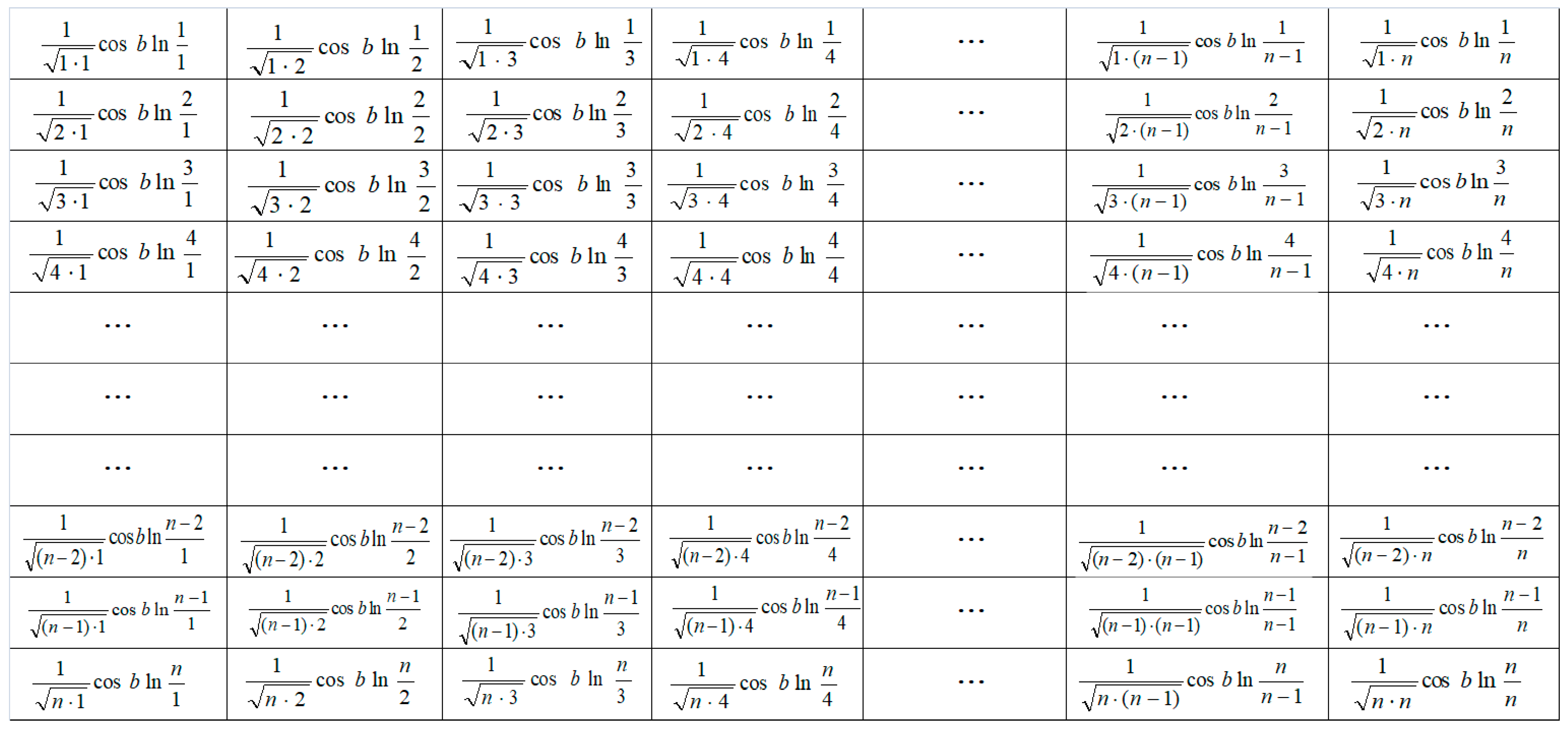
Theorem 1.

Assume b ∈ ℝ is such that ζ(1/2 + ib) = 0, where ζ(s) is the Riemann zeta function. Let A₂ denote the series of complex numbers defined by Equation (30), and let G_tot denote the real number series obtained by summing the entries of all cells in the square n × n matrix of Figure 1. Then, within the representative framework and in the asymptotic regime n → ∞, the formal identity G_tot − |A₂|² = 0 is obtained.

$$A_2=1^{-s}+2^{-s}+3^{-s}+\dots +n^{-s}+\dots$$

(30)

Figure 1 represents an n × n matrix depending on the parameter b, whose entries are given explicitly and define the finite quantity G_tot(n) as the sum of all its elements.

Figure 1. An n × n matrix.

Figure 1. An n × n matrix.

Proof. 

The complex-valued series A₂, defined by Equation (30) with s = a + ib, coincides with the Dirichlet series representation of ζ(s). This series is divergent for α < 1, and in particular for a = 1/2. By employing infinite numbers, Equation (30) admits the following representation within the infinite number framework

$$A_2(\xi )=1^{-s}+2^{-s}+3^{-s}+\dots +{\xi }^{-s}$$

(31)

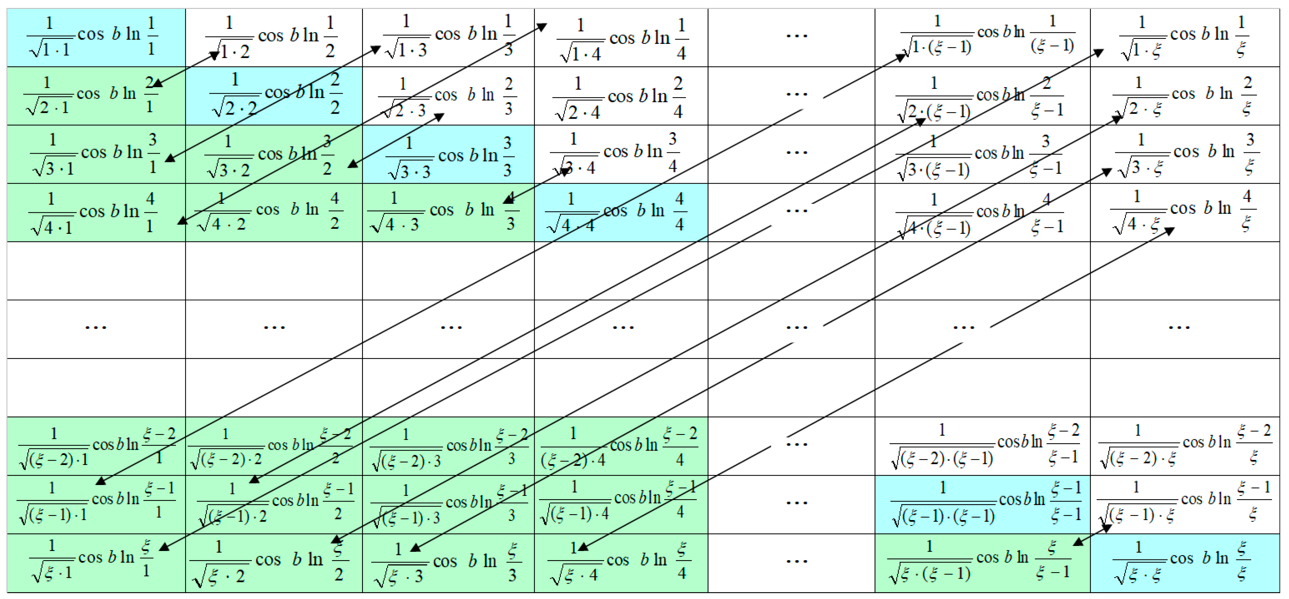
Furthermore, as n → ∞, the matrix in Figure 1 admits a formal representative counterpart in Figure 2, obtained by replacing n with the infinite unit ξ. Let us now consider Equation (12), restated below as Equation (32)

$$G(\xi )=2\left({\displaystyle \frac{1}{\sqrt{1\cdot 2}}}\cos \left(b\ln {\displaystyle \frac{1}{2}}\right)+\dots +{\displaystyle \frac{1}{\sqrt{1\cdot \xi }}}\cos \left(b\ln {\displaystyle \frac{1}{\xi }}\right)+{\displaystyle \frac{1}{\sqrt{2\cdot 3}}}\cos \left(b\ln {\displaystyle \frac{2}{3}}\right)+\dots +{\displaystyle \frac{1}{\sqrt{2\cdot \xi }}}\cos \left(b\ln {\displaystyle \frac{2}{\xi }}\right)+\dots +{\displaystyle \frac{1}{\sqrt{(\xi -1)\cdot \xi }}}\cos \left(b\ln {\displaystyle \frac{(\xi -1)}{\xi }}\right)\right)$$

(32)

It is observed that the series in Equation (32) consists of the sum of the entries (with a white background) of the square matrix in Figure 2, which are located to the right of the main diagonal. Upon completion of the missing terms in series (32), these additional terms correspond to the entries with colored backgrounds (green or blue) in Figure 2. Furthermore, each entry with a green background is equal to its symmetric counterpart (with white background), as indicated by the corresponding bidirectional arrows. For example: ${\displaystyle \frac{1}{\sqrt{2\cdot 1}}}\cos b\ln {\displaystyle \frac{2}{1}}={\displaystyle \frac{1}{\sqrt{1\cdot 2}}}\cos b\ln {\displaystyle \frac{1}{2}}$. Additionally, the entries along the main diagonal (with blue background) all involve cosine terms whose values are equal to unity. Thus, for instance, ${\displaystyle \frac{1}{\sqrt{1\cdot 1}}}\cos b\ln {\displaystyle \frac{1}{1}}={\displaystyle \frac{1}{1}}$, and ${\displaystyle \frac{1}{\sqrt{2\cdot 2}}}\cos b\ln {\displaystyle \frac{2}{2}}={\displaystyle \frac{1}{2}}$, and ${\displaystyle \frac{1}{\sqrt{3\cdot 3}}}\cos b\ln {\displaystyle \frac{3}{3}}={\displaystyle \frac{1}{3}}$, and so forth. Finally, since the series in Equation (32) includes a factor of two, the complete series G_tot corresponding to the matrix in Figure 2 is given by G(ξ) plus the sum of the diagonal terms. Consequently, the formal relation (33) is obtained

$$G_{tot}=G(\xi )+\left({\displaystyle \frac{1}{1}}+{\displaystyle \frac{1}{2}}+\dots +{\displaystyle \frac{1}{\xi }}\right)$$

(33)

By comparing Equation (33) with Equation (11)— restated below as Equation (34) for convenience—which holds when the values of b correspond to nontrivial zeros of the Riemann zeta function ζ(s), we observe that, within the representative interpretation, the complete series G_tot may be identified formally with |A₂(ξ)|²

$$\left|A_2(\xi )\right|=\sqrt{\left({\displaystyle \frac{1}{1}}+{\displaystyle \frac{1}{2}}+\dots +{\displaystyle \frac{1}{\xi }}\right)+G(\xi )}$$

(34)

The matrix in Figure 2 shows the representative asymptotic counterpart of Figure 1, obtained by formally replacing the finite parameter n with the infinite unit ξ. Its entries are interpreted within the representative framework and are used only in this formal asymptotic sense.

Consequently, whenever b $\in$ ℝ satisfies ζ(1/2 + ib) = 0, the representative formal identity G_tot − |A₂|² = 0 is obtained. This identity is to be interpreted strictly within the infinite number representative framework. It extends the corresponding finite-n identity to the asymptotic representative setting and is not intended as an independent summation rule for divergent series in the classical sense. □

Remark 3.

For every finite n, the identity G_tot(n) = |A₂(n)|² follows directly from the outer-product structure of the entries of the matrix in Figure 1, since

$${\displaystyle \sum _{j=1}^n{\displaystyle \sum _{k=1}^n{j}^{-s}{k}^{-\overline{s}}=}}\left({\displaystyle \sum _{j=1}^n{j}^{-s}}\right)\left({\displaystyle \sum _{k=1}^n{k}^{-\overline{s}}}\right)$$

The infinite number formulation provides a consistent extension of this finite identity to the divergent regime α ≤ 1, where the classical Dirichlet series no longer converges.

Theorem 2.

If b ∈ ℝ is the imaginary part of any nontrivial zero of the Riemann zeta function ζ(s) lying on the critical line, then within the representative framework the following formal relation is derived, where γ denotes the Euler–Mascheroni constant.

$$\begin{gathered} \underset{n\to +\infty }{\lim }\left\{{\displaystyle \frac{1}{\sqrt{1\cdot 2}}}\cos \left(b\ln {\displaystyle \frac{1}{2}}\right)+\dots +{\displaystyle \frac{1}{\sqrt{1\cdot n}}}\cos \left(b\ln {\displaystyle \frac{1}{n}}\right)+{\displaystyle \frac{1}{\sqrt{2\cdot 3}}}\cos \left(b\ln {\displaystyle \frac{2}{3}}\right)+\dots +{\displaystyle \frac{1}{\sqrt{2\cdot n}}}\cos \left(b\ln {\displaystyle \frac{2}{n}}\right)+\dots +{\displaystyle \frac{1}{\sqrt{(n-1)\cdot n}}}\cos \left(b\ln {\displaystyle \frac{(n-1)}{n}}\right)\right. \\ \left.-{\displaystyle \frac{\sqrt{1+4b^2}}{1-4b^2}}{n}^{-a+1}\cdot \left[{\displaystyle \frac{1}{\sqrt{1}}}\sin \left(b\ln {\displaystyle \frac{1}{n}}+\mathrm{atan}{\displaystyle \frac{1}{2b}}\right)+{\displaystyle \frac{1}{\sqrt{2}}}\sin \left(b\ln {\displaystyle \frac{2}{n}}+\mathrm{atan}{\displaystyle \frac{1}{2b}}\right)+\dots +{\displaystyle \frac{1}{\sqrt{n}}}\sin \left(b\ln {\displaystyle \frac{n}{n}}+\mathrm{atan}{\displaystyle \frac{1}{2b}}\right)\right]+{\displaystyle \frac{\ln (n)}{2}}\right\}=-{\displaystyle \frac{\gamma }{2}} \end{gathered}$$

(35)

Proof. 

Within the representative framework of infinite numbers, Equation (35) is formally rewritten as Equation (36), where G(ξ) denotes the same quantity as in Equations (32)–(34) of Theorem 1. Since Equation (35) holds identically for every finite n, its reformulation in terms of the infinite unit ξ represents an algebraically equivalent infinite number expression.

$$\begin{gathered} G(\xi )=2\left({\displaystyle \frac{1}{\sqrt{1\cdot 1}}}\cos \left(b\ln {\displaystyle \frac{1}{2}}\right)+\dots +{\displaystyle \frac{1}{\sqrt{1\cdot \xi }}}\cos \left(b\ln {\displaystyle \frac{1}{\xi }}\right)+{\displaystyle \frac{1}{\sqrt{2\cdot 3}}}\cos \left(b\ln {\displaystyle \frac{2}{3}}\right)+\dots +{\displaystyle \frac{1}{\sqrt{2\cdot \xi }}}\cos \left(b\ln {\displaystyle \frac{2}{\xi }}\right)+\dots +{\displaystyle \frac{1}{\sqrt{(\xi -1)\cdot \xi }}}\cos \left(b\ln {\displaystyle \frac{(\xi -1)}{\xi }}\right)\right) \\ =2{\displaystyle \frac{\sqrt{(1/4+b^2}}{1/4-b^2}}{\xi }^{-a+1}\cdot \left[{\displaystyle \frac{1}{\sqrt{1}}}\sin \left(b\ln {\displaystyle \frac{1}{\xi }}+\mathrm{atan}{\displaystyle \frac{1}{2b}}\right)+{\displaystyle \frac{1}{\sqrt{2}}}\sin \left(b\ln {\displaystyle \frac{2}{\xi }}+\mathrm{atan}{\displaystyle \frac{1}{2b}}\right)+\dots +{\displaystyle \frac{1}{\sqrt{\xi }}}\sin \left(b\ln {\displaystyle \frac{\xi }{\xi }}+\mathrm{atan}{\displaystyle \frac{1}{2b}}\right)\right]-\ln (\xi )-\gamma \end{gathered}$$

(36)

Given that the derivative of an infinite number series-representation is determined by its last infinite term (in the infinite number sense; cf. [4]), differentiating Equation (33) of Theorem 1 yields Equation (37), where α = 1/2

$${\displaystyle \frac{d{G}_{tot}}{d\xi }}={\displaystyle \frac{dG}{d\xi }}+{\displaystyle \frac{1}{\xi }}={\displaystyle \frac{dG}{d\xi }}+{\displaystyle \frac{1}{{\xi }^{2\alpha }}}$$

(37)

On the other hand, the derivative of the infinite number function G_tot(ξ), which represents the complete series described in Theorem 1, is equal to the sum of the derivatives of the individual series, each corresponding to a row of the matrix in Figure 2. Consequently, the derivative of G_tot(ξ) is given by the sum of the entries in the last column of the matrix in Figure 2. Therefore, Equation (38) follows.

$$\begin{gathered} {\displaystyle \frac{d{G}_{tot}}{d\xi }}=\left({\displaystyle \frac{1}{\sqrt{1\cdot \xi }}}\cos b\ln {\displaystyle \frac{1}{\xi }}+{\displaystyle \frac{1}{\sqrt{2\cdot \xi }}}\cos b\ln {\displaystyle \frac{2}{\xi }}+\dots +{\displaystyle \frac{1}{\sqrt{\xi \cdot \xi }}}\cos b\ln {\displaystyle \frac{\xi }{\xi }}\right) \\ =\left({\displaystyle \frac{1}{1^a{\xi }^a}}\cos b\ln {\displaystyle \frac{1}{\xi }}+{\displaystyle \frac{1}{2^a{\xi }^a}}\cos b\ln {\displaystyle \frac{2}{\xi }}+\dots +{\displaystyle \frac{1}{{\xi }^a{\xi }^a}}\cos b\ln {\displaystyle \frac{\xi }{\xi }}\right)\hspace{1em}\hspace{1em}\hspace{1em}\hspace{1em}\mathrm{where} \alpha =1/2 \end{gathered}$$

(38)

Taking Equation (38) into account, Equation (37) becomes Equation (39)

$${\displaystyle \frac{dG}{d\xi }}=\left({\displaystyle \frac{1}{1^a{\xi }^a}}\cos b\ln {\displaystyle \frac{1}{\xi }}+{\displaystyle \frac{1}{2^a{\xi }^a}}\cos b\ln {\displaystyle \frac{2}{\xi }}+\dots +{\displaystyle \frac{1}{{\xi }^a{\xi }^a}}\cos b\ln {\displaystyle \frac{\xi }{\xi }}\right)-{\displaystyle \frac{1}{{\xi }^{2a}}}$$

(39)

Therefore, to calculate G(ξ) the integral of the above Equation (39) is taken

$$\begin{gathered} G=G(\xi )={\displaystyle \int \left(\frac{1}{1^a{\xi }^a}\cos b\ln \frac{1}{\xi }+\frac{1}{2^a{\xi }^a}\cos b\ln \frac{2}{\xi }+\dots +\frac{1}{{\xi }^a{\xi }^a}\cos b\ln \frac{\xi }{\xi }\right)d\xi }-{\displaystyle \int \frac{1}{{\xi }^{2a}}d\xi } \\ ={\displaystyle \frac{1}{1^a}}{\displaystyle \int \left(\frac{1}{{\xi }^a}\cos b\ln \frac{1}{\xi }\right)d\xi }+{\displaystyle \frac{1}{2^a}}{\displaystyle \int \left(\frac{1}{{\xi }^a}\cos b\ln \frac{2}{\xi }\right)d\xi }+\dots +{\displaystyle \frac{1}{{\xi }^a}}{\displaystyle \int \left(\frac{1}{{\xi }^a}\cos b\ln \frac{\xi }{\xi }\right)d\xi }-{\displaystyle \int \frac{1}{{\xi }^{2a}}d\xi } \end{gathered}$$

(40)

$={\displaystyle \frac{1}{1^a}}{\mathrm{{\rm I}}}_1+{\displaystyle \frac{1}{2^a}}{\mathrm{{\rm I}}}_2+\dots +{\displaystyle \frac{1}{{\xi }^a}}{\mathrm{{\rm I}}}_{\xi }-{\displaystyle \int \frac{1}{{\xi }^{2a}}d\xi }$, where Ι₁, Ι₂, …, Ι_ξ denote the corresponding integrals given above.

Moreover, it holds that ${\displaystyle \int \frac{1}{{\xi }^{2a}}d\xi }={\displaystyle \frac{{\xi }^{-2a+1}}{-2\alpha +1}}+C$, where C is a finite constant. Clearly, C = C′; that is, the constant C is identical to the constant C′ appearing in Equation (16), since both arise from the same integral (see Equation (16)). Therefore, we have

$$G={\displaystyle \frac{1}{1^a}}{\mathrm{{\rm I}}}_1+{\displaystyle \frac{1}{2^a}}{\mathrm{{\rm I}}}_2+\dots +{\displaystyle \frac{1}{{\xi }^a}}{\mathrm{{\rm I}}}_{\xi }-{\displaystyle \frac{{\xi }^{-2a+1}}{-2\alpha +1}}-C^{\prime }$$

(41)

Taking into account Equation (22), which is repeated below, for convenience reasons

$${\displaystyle \int f^{\prime }(x)g(x)dx}=f(x)g(x)-{\displaystyle \int f(x)g^{\prime }(x)dx}$$

(42)

we have

$$\begin{gathered} {\mathrm{{\rm I}}}_1={\displaystyle \int \left(\frac{1}{{\xi }^a}\cos b\ln \frac{1}{\xi }\right)d\xi }={\displaystyle \int {\left(\frac{{\xi }^{-a+1}}{-\alpha +1}\right)}^{\prime }\cos b\ln \frac{1}{\xi }d\xi }={\displaystyle \frac{{\xi }^{-a+1}}{-\alpha +1}}\cos b\ln {\displaystyle \frac{1}{\xi }}-{\displaystyle \int \frac{{\xi }^{-a+1}}{-\alpha +1}{\left(\cos b\ln \frac{1}{\xi }\right)}^{\prime }d\xi } \\ ={\displaystyle \frac{{\xi }^{-a+1}}{-\alpha +1}}\cos b\ln {\displaystyle \frac{1}{\xi }}-{\displaystyle \int \frac{{\xi }^{-a+1}}{-\alpha +1}\left(-\sin b\ln \frac{1}{\xi }\right)\cdot \left(-\frac{b}{\xi }\right)d\xi }={\displaystyle \frac{{\xi }^{-a+1}}{-\alpha +1}}\cos b\ln {\displaystyle \frac{1}{\xi }}-{\displaystyle \frac{b}{-\alpha +1}}{\displaystyle \int {\xi }^{-a}\left(\sin b\ln \frac{1}{\xi }\right)d\xi } \end{gathered}$$

(43)

However, the last integral in Equation (43) transforms as follows:

$$\begin{gathered} {\displaystyle \int \left(\frac{1}{{\xi }^a}\sin b\ln \frac{1}{\xi }\right)d\xi }={\displaystyle \int {\left(\frac{{\xi }^{-a+1}}{-\alpha +1}\right)}^{\prime }\sin b\ln \frac{1}{\xi }d\xi }={\displaystyle \frac{{\xi }^{-a+1}}{-\alpha +1}}\sin b\ln {\displaystyle \frac{1}{\xi }}-{\displaystyle \int \frac{{\xi }^{-a+1}}{-\alpha +1}{\left(\sin b\ln \frac{1}{\xi }\right)}^{\prime }d\xi } \\ ={\displaystyle \frac{{\xi }^{-a+1}}{-\alpha +1}}\sin b\ln {\displaystyle \frac{1}{\xi }}-{\displaystyle \int \frac{{\xi }^{-a+1}}{-\alpha +1}\left(\cos b\ln \frac{1}{\xi }\right)\cdot \left(-\frac{b}{\xi }\right)d\xi }={\displaystyle \frac{{\xi }^{-a+1}}{-\alpha +1}}\sin b\ln {\displaystyle \frac{1}{\xi }}-{\displaystyle \frac{b}{-\alpha +1}}{\displaystyle \int {\xi }^{-a}\left(\cos b\ln \frac{1}{\xi }\right)d\xi } \\ ={\displaystyle \frac{{\xi }^{-a+1}}{-\alpha +1}}\sin b\ln {\displaystyle \frac{1}{\xi }}-{\displaystyle \frac{b}{-\alpha +1}}{I}_1 \end{gathered}$$

(44)

Therefore, from Equations (43) and (44), it follows that

$$\begin{gathered} {\mathrm{{\rm I}}}_1={\displaystyle \frac{{\xi }^{-a+1}}{-\alpha +1}}\cos b\ln {\displaystyle \frac{1}{\xi }}-{\displaystyle \frac{b}{-\alpha +1}}{\displaystyle \int {\xi }^{-a}\left(\sin b\ln \frac{1}{\xi }\right)d\xi } \\ ={\displaystyle \frac{{\xi }^{-a+1}}{-\alpha +1}}\cos b\ln {\displaystyle \frac{1}{\xi }}-{\displaystyle \frac{b}{-\alpha +1}}\left({\displaystyle \frac{{\xi }^{-a+1}}{-\alpha +1}}\sin b\ln {\displaystyle \frac{1}{\xi }}-{\displaystyle \frac{b}{-\alpha +1}}{I}_1\right) \Rightarrow \\ {\mathrm{{\rm I}}}_1={\displaystyle \frac{{\xi }^{-a+1}}{-\alpha +1}}\cos b\ln {\displaystyle \frac{1}{\xi }}-{\displaystyle \frac{b}{{(-\alpha +1)}^2}}{\xi }^{-a+1}\sin b\ln {\displaystyle \frac{1}{\xi }}+{\displaystyle \frac{b^2}{{(-\alpha +1)}^2}}{I}_1 \\ {\displaystyle \frac{{(-\alpha +1)}^2-b^2}{{(-\alpha +1)}^2}}{\mathrm{{\rm I}}}_1={\displaystyle \frac{{\xi }^{-a+1}}{-\alpha +1}}\cos b\ln {\displaystyle \frac{1}{\xi }}-{\displaystyle \frac{b}{{(-\alpha +1)}^2}}{\xi }^{-a+1}\sin b\ln {\displaystyle \frac{1}{\xi }} \Rightarrow \\ {\mathrm{{\rm I}}}_1={\displaystyle \frac{1-\alpha }{{(1-\alpha )}^2-b^2}}{\xi }^{-a+1}\cos b\ln {\displaystyle \frac{1}{\xi }}+{\displaystyle \frac{b}{{(1-\alpha )}^2-b^2}}{\xi }^{-a+1}\sin b\ln {\displaystyle \frac{1}{\xi }}+{C_1}^{*} \\ ={\xi }^{-a+1}\left({\displaystyle \frac{1-\alpha }{{(1-\alpha )}^2-b^2}}\cos b\ln {\displaystyle \frac{1}{\xi }}+{\displaystyle \frac{b}{{(1-\alpha )}^2-b^2}}\sin b\ln {\displaystyle \frac{1}{\xi }}\right)+{C_1}^{*} \end{gathered}$$

(45)

Now, according to Equation (43) it follows that $\left\{{\displaystyle \frac{d{\mathrm{{\rm I}}}_1}{d\xi }}={\displaystyle \frac{d}{d\xi }}{\displaystyle \int \left(\frac{1}{{\xi }^a}\cos b\ln \frac{1}{\xi }\right)d\xi }\right.\left.={\displaystyle \frac{1}{{\xi }^a}}\cos b\ln {\displaystyle \frac{1}{\xi }}=0\right\}$ given that α = 1/2. Therefore, ${\displaystyle \frac{d{\mathrm{{\rm I}}}_1}{d\xi }}=0$, and taken Equation (45) into account, and furthermore assuming $L_1={\displaystyle \frac{1-\alpha }{{(1-\alpha )}^2-b^2}}$ and $L_2={\displaystyle \frac{b}{{(1-\alpha )}^2-b^2}}$, we obtain

$${\displaystyle \frac{d{\mathrm{{\rm I}}}_1}{d\xi }}={\displaystyle \frac{1}{2\sqrt{\xi }}}\left(L_1\cos \left(b\ln {\displaystyle \frac{1}{\xi }}\right)+L_2\sin \left(b\ln {\displaystyle \frac{1}{\xi }}\right)\right)+\sqrt{\xi }\left(-L_{1}b\left(-{\displaystyle \frac{1}{\xi }}\right)\sin \left(b\ln {\displaystyle \frac{1}{\xi }}\right)+L_{2}b\left(-{\displaystyle \frac{1}{\xi }}\right)\cos \left(b\ln {\displaystyle \frac{1}{\xi }}\right)\right)+{\displaystyle \frac{d{C_1}^{*}}{d\xi }}=0$$

Thus

$$\begin{gathered} {\displaystyle \frac{1}{2\sqrt{\xi }}}\left(L_1\cos \left(b\ln {\displaystyle \frac{1}{\xi }}\right)+L_2\sin \left(b\ln {\displaystyle \frac{1}{\xi }}\right)\right)+{\displaystyle \frac{1}{\sqrt{\xi }}}\left(L_{1}b\sin \left(b\ln {\displaystyle \frac{1}{\xi }}\right)-L_{2}b\cos \left(b\ln {\displaystyle \frac{1}{\xi }}\right)\right)+{\displaystyle \frac{d{C_1}^{*}}{d\xi }}=0\Rightarrow \\ {\displaystyle \frac{d{C_1}^{*}}{d\xi }}=0 \end{gathered}$$

(46)

Therefore, we obtain that ${\displaystyle \frac{d{C_1}^{*}}{d\xi }}=0$, which means that ${C_1}^{*}$ is a finite number, and not a function of ξ.

Moreover, it is well known that Equation (45)—being the sum of two sinusoidal functions—can further be expressed as a simple sine function, namely as Equation (47)

$${\mathrm{{\rm I}}}_1={\xi }^{-a+1}\cdot A\sin \left(b\ln {\displaystyle \frac{1}{\xi }}+\varphi \right)+{C_1}^{*}$$

(47)

where

$$A=\sqrt{{\left({\displaystyle \frac{1-\alpha }{{(1-\alpha )}^2-b^2}}\right)}^2+{\left({\displaystyle \frac{b}{{(1-\alpha )}^2-b^2}}\right)}^2}={\displaystyle \frac{\sqrt{{(1-\alpha )}^2+b^2}}{{(1-\alpha )}^2-b^2}}$$

(48)

$$\mathrm{and}\hspace{1em}\hspace{1em}\hspace{1em}\varphi =\mathrm{atan}{\displaystyle \frac{\frac{1-\alpha }{{(1-\alpha )}^2-b^2}}{\frac{b}{{(1-\alpha )}^2-b^2}}}=\mathrm{atan}{\displaystyle \frac{1-\alpha }{b}}$$

(49)

Therefore:

$${\displaystyle \frac{1}{1^a}}{\mathrm{{\rm I}}}_1={\displaystyle \frac{{\xi }^{-a+1}}{1^a}}\cdot {\displaystyle \frac{\sqrt{{(1-\alpha )}^2+b^2}}{{(1-\alpha )}^2-b^2}}\sin \left(b\ln {\displaystyle \frac{1}{\xi }}+\mathrm{atan}{\displaystyle \frac{1-\alpha }{b}}\right)+{\displaystyle \frac{1}{1^a}}{C_1}^{*}$$

(50)

In a similar manner, it follows that

$$\begin{gathered} {\mathrm{{\rm I}}}_2={\displaystyle \int \left(\frac{1}{{\xi }^a}\cos b\ln \frac{2}{\xi }\right)d\xi }={\displaystyle \int {\left(\frac{{\xi }^{-a+1}}{-\alpha +1}\right)}^{\prime }\cos b\ln \frac{2}{\xi }d\xi }={\displaystyle \frac{{\xi }^{-a+1}}{-\alpha +1}}\cos b\ln {\displaystyle \frac{2}{\xi }}-{\displaystyle \int \frac{{\xi }^{-a+1}}{-\alpha +1}{\left(\cos b\ln \frac{2}{\xi }\right)}^{\prime }d\xi } \\ ={\displaystyle \frac{{\xi }^{-a+1}}{-\alpha +1}}\cos b\ln {\displaystyle \frac{2}{\xi }}-{\displaystyle \int \frac{{\xi }^{-a+1}}{-\alpha +1}\left(-\sin b\ln \frac{2}{\xi }\right)\cdot \left(-\frac{b}{\xi }\right)d\xi }={\displaystyle \frac{{\xi }^{-a+1}}{-\alpha +1}}\cos b\ln {\displaystyle \frac{2}{\xi }}-{\displaystyle \frac{b}{-\alpha +1}}{\displaystyle \int {\xi }^{-a}\left(\sin b\ln \frac{2}{\xi }\right)d\xi } \\ {\mathrm{{\rm I}}}_2={\displaystyle \frac{{\xi }^{-a+1}}{-\alpha +1}}\cos b\ln {\displaystyle \frac{2}{\xi }}-{\displaystyle \frac{b}{-\alpha +1}}{\displaystyle \int {\xi }^{-a}\left(\sin b\ln \frac{2}{\xi }\right)d\xi }+{C_2}^{*} \end{gathered}$$

After carrying out the corresponding calculations, we similarly obtain

$${\displaystyle \frac{1}{2^a}}{\mathrm{{\rm I}}}_2={\displaystyle \frac{{\xi }^{-a+1}}{2^a}}\cdot {\displaystyle \frac{\sqrt{{(1-\alpha )}^2+b^2}}{{(1-\alpha )}^2-b^2}}\sin \left(b\ln {\displaystyle \frac{2}{\xi }}+\mathrm{atan}{\displaystyle \frac{1-\alpha }{b}}\right)+{C_2}^{*}$$

(51)

Finally, it holds that

$${\displaystyle \frac{1}{{\xi }^a}}{\mathrm{{\rm I}}}_{\xi }={\displaystyle \frac{{\xi }^{-a+1}}{{\xi }^a}}\cdot {\displaystyle \frac{\sqrt{{(1-\alpha )}^2+b^2}}{{(1-\alpha )}^2-b^2}}\sin \left(b\ln {\displaystyle \frac{\xi }{\xi }}+\mathrm{atan}{\displaystyle \frac{1-\alpha }{b}}\right)+{C_{\mathrm{\xi }}}^{*}$$

(52)

Hence, by applying Equations (50)–(52), Equation (41) takes the following form

$$G={\displaystyle \frac{\sqrt{{(1-\alpha )}^2+b^2}}{{(1-\alpha )}^2-b^2}}{\xi }^{-a+1}\cdot \left[{\displaystyle \frac{1}{1^a}}\sin \left(b\ln {\displaystyle \frac{1}{\xi }}+\mathrm{atan}{\displaystyle \frac{1-\alpha }{b}}\right)+{\displaystyle \frac{1}{2^a}}\sin \left(b\ln {\displaystyle \frac{2}{\xi }}+\mathrm{atan}{\displaystyle \frac{1-\alpha }{b}}\right)+\dots +{\displaystyle \frac{1}{{\xi }^a}}\sin \left(b\ln {\displaystyle \frac{\xi }{\xi }}+\mathrm{atan}{\displaystyle \frac{1-\alpha }{b}}\right)\right]-{\displaystyle \frac{{\xi }^{-2a+1}}{-2\alpha +1}}-C^{*}$$

(53)

where $C^{*}=C^{\prime }-{C_1}^{*}-{C_2}^{*}-\dots -{C_{\mathrm{\xi }}}^{*}$.

However, according to Lemma 1, and taking into account that α = 1/2, the series inside the parenthesis in Equation (53) is:

$${\mathrm{\Sigma }}_{\infty }={\displaystyle \frac{1}{1^a}}\sin \left(b\ln {\displaystyle \frac{1}{\xi }}+\mathrm{atan}{\displaystyle \frac{1-\alpha }{b}}\right)+{\displaystyle \frac{1}{2^a}}\sin \left(b\ln {\displaystyle \frac{2}{\xi }}+\mathrm{atan}{\displaystyle \frac{1-\alpha }{b}}\right)+\dots +{\displaystyle \frac{1}{{\xi }^a}}\sin \left(b\ln {\displaystyle \frac{\xi }{\xi }}+\mathrm{atan}{\displaystyle \frac{1-\alpha }{b}}\right)=2{\displaystyle \frac{1-4b^2}{{(1+4b^2)}^{3/2}}}\sqrt{\xi }+C_b$$

(54)

Hence, Equation (53) can be rewritten as:

$$G={\displaystyle \frac{\sqrt{{(1-\alpha )}^2+b^2}}{{(1-\alpha )}^2-b^2}}{\xi }^{-a+1}\cdot \left(2{\displaystyle \frac{1-4b^2}{{(1+4b^2)}^{3/2}}}\sqrt{\xi }+C_b\right)-{\displaystyle \frac{{\xi }^{-2a+1}}{-2\alpha +1}}-C^{*}$$

(55)

Furthermore, considering that α = 1/2, Equation (55) is finally transformed into Equation (56)

$$G={\displaystyle \frac{4\xi }{1+4b^2}}+C_b{\displaystyle \frac{2\sqrt{1+4b^2}}{1-4b^2}}\sqrt{\xi }-{\displaystyle \frac{{\xi }^0}{0}}-C^{*}$$

(56)

However, as established in [17], for α = 1/2, and values of b $\in$ ℝ corresponding to any nontrivial zero of the Riemann zeta function ζ(s) lying on the critical line, Equation (17) is valid and is restated below as Equation (57)

$$G={\displaystyle \frac{4\xi }{1+4b^2}}-\ln \xi -\gamma$$

(57)

By comparing Equations (56) and (57), we impose formal compatibility between the two representative expressions within the normal-form conventions adopted in the present framework. In this comparison, logarithmic and algebraic terms (e.g., lnξ, ξ, √ξ) are treated as asymptotically independent components. Formal compatibility therefore requires matching the corresponding coefficients at each asymptotic order.

Accordingly, the asymptotic orders are matched, and the two representations are regarded as formally compatible within the representative framework. To this end, we make the following observations: (i) First, we note that the term with ξ raised to the first power, namely the expression ${\displaystyle \frac{4\xi }{1+4b^2}}$ is identical in both Equations (56) and (57). (ii) Moreover, we observe that the term with ξ raised to the power ½, namely the term $C_b{\displaystyle \frac{2\sqrt{1+4b^2}}{1-4b^2}}\sqrt{\xi }$ in Equation (56), does not appear in Equation (57) implying that the finite number C_b should be zero. Since no √ξ term appears in Equation (57), consistency requires the coefficient of √ξ in Equation (56) to vanish. Indeed, as the representation is in normal form with respect to powers of ξ (cf. [4]), a term in ξ^1/2 cannot be absorbed into terms of different order; therefore its coefficient must be zero. (iii) Furthermore, it is necessary that the terms without ξ be the same, that is C* = γ. (iv) Finally, regarding the remaining terms, the relation (${\displaystyle \frac{{\xi }^0}{0}}=\ln \xi$) must hold. In the present framework, quantities formally identified with zero in asymptotic expressions are interpreted as infinitesimal terms. To determine whether such a term is infinitesimal, it may be parametrized by an auxiliary variable t(ξ), representing a generic infinite number contribution. Consistency of the representation then requires that this contribution be infinitesimal.

This relation is transformed as follows:

$$\begin{gathered} {\xi }^t=t\ln \xi \Rightarrow \ln ({\xi }^t)=\ln (t\ln \xi )=\ln t+\ln (\ln \xi )\Rightarrow t\ln \xi =\ln t+\ln (\ln \xi )\Rightarrow \\ t\ln \xi -\ln t=\ln (\ln \xi ) \end{gathered}$$

(58)

Equation (58) is of the form $At-\ln t={\rm B}$ where coefficients A and B are, respectively, A = lnξ and B = ln(lnξ). As is well known, this equation admits a solution in the form $t={\displaystyle \frac{1}{A}}W\left({\displaystyle \frac{A}{e^{{\rm B}}}}\right)$, where W denotes the Lambert function (also referred to as the omega function). Therefore, by substituting the values of A and B, we obtain

$$t={\displaystyle \frac{1}{\ln \xi }}W\left({\displaystyle \frac{\ln \xi }{e^{\ln (\ln \xi )}}}\right)={\displaystyle \frac{1}{\ln \xi }}W\left({\displaystyle \frac{\ln \xi }{\ln \xi }}\right)={\displaystyle \frac{1}{\ln \xi }}W\left(1\right)$$

(59)

The value of the Lambert function W(z) for z = 1 on the principal branch is W(1) = 0.567143… In other words, the value (w) that satisfies the equation $w{e}^w=1$ is w = 0.567143…Hence, Equation (59) can be equivalently rewritten as Equation (60), thereby confirming that the infinite number (t) in Equation (58) is indeed equal to zero.

$$t={\displaystyle \frac{1}{\ln \xi }}W\left({\displaystyle \frac{\ln \xi }{e^{\ln (\ln \xi )}}}\right)={\displaystyle \frac{1}{\ln \xi }}\cdot 0.567143\dots =0$$

(60)

Furthermore, for z = 1, all branches W_k(1) of the Lambert function are finite complex constants. Hence, from Equation (59), we obtain

$$t={\displaystyle \frac{W_k\left(1\right)}{\ln \xi }}$$

which implies that t scales as a finite constant divided by lnξ and therefore represents an infinitesimal quantity for every fixed branch index k. Consequently, consistency of the asymptotic representation requires t = 0 within the representative framework. The use of the Lambert W function in this context serves only to resolve the asymptotic scaling of the infinitesimal parameter and does not introduce additional analytical assumptions.

Therefore, within the representative framework, Equations (56) and (57) are formally compatible, and the findings of the present study are consistent with the corresponding representative relations reported in [17].

Thus, based on the above, considering that C* =γ, ${\displaystyle \frac{{\xi }^{-2a+1}}{-2\alpha +1}}=\ln \xi$, and α = 1/2, Equation (53) can be written

$$\begin{gathered} G={\displaystyle \frac{\sqrt{{(1-\alpha )}^2+b^2}}{{(1-\alpha )}^2-b^2}}{\xi }^{-a+1}\cdot \left[{\displaystyle \frac{1}{1^a}}\sin \left(b\ln {\displaystyle \frac{1}{\xi }}+\mathrm{atan}{\displaystyle \frac{1-\alpha }{b}}\right)+{\displaystyle \frac{1}{2^a}}\sin \left(b\ln {\displaystyle \frac{2}{\xi }}+\mathrm{atan}{\displaystyle \frac{1-\alpha }{b}}\right)+\dots +{\displaystyle \frac{1}{{\xi }^a}}\sin \left(b\ln {\displaystyle \frac{\xi }{\xi }}+\mathrm{atan}{\displaystyle \frac{1-\alpha }{b}}\right)\right]-\ln \xi -\mathsf{\gamma } \\ =2{\displaystyle \frac{\sqrt{1+4b^2}}{1-4b^2}}\sqrt{\xi }\cdot \left[{\displaystyle \frac{1}{\sqrt{1}}}\sin \left(b\ln {\displaystyle \frac{1}{\xi }}+\mathrm{atan}{\displaystyle \frac{1}{2b}}\right)+{\displaystyle \frac{1}{\sqrt{2}}}\sin \left(b\ln {\displaystyle \frac{2}{\xi }}+\mathrm{atan}{\displaystyle \frac{1}{2b}}\right)+\dots +{\displaystyle \frac{1}{\sqrt{\xi }}}\sin \left(b\ln {\displaystyle \frac{\xi }{\xi }}+\mathrm{atan}{\displaystyle \frac{1}{2b}}\right)\right]-\ln \xi -\mathsf{\gamma } \end{gathered}$$

(61)

Moreover, taking into account the analytical expression of G, as shown in Equation (32), Equation (61) is transformed into

$$\begin{gathered} {\displaystyle \frac{G}{2}}=\left({\displaystyle \frac{1}{\sqrt{1\cdot 2}}}\cos \left(b\ln {\displaystyle \frac{1}{2}}\right)+\dots +{\displaystyle \frac{1}{\sqrt{1\cdot \xi }}}\cos \left(b\ln {\displaystyle \frac{1}{\xi }}\right)+{\displaystyle \frac{1}{\sqrt{2\cdot 3}}}\cos \left(b\ln {\displaystyle \frac{2}{3}}\right)+\dots +{\displaystyle \frac{1}{\sqrt{2\cdot \xi }}}\cos \left(b\ln {\displaystyle \frac{2}{\xi }}\right)+\dots +{\displaystyle \frac{1}{\sqrt{(\xi -1)\cdot \xi }}}\cos \left(b\ln {\displaystyle \frac{(\xi -1)}{\xi }}\right)\right) \\ ={\displaystyle \frac{\sqrt{1+4b^2}}{1-4b^2}}\sqrt{\xi }\cdot \left[{\displaystyle \frac{1}{\sqrt{1}}}\sin \left(b\ln {\displaystyle \frac{1}{\xi }}+\mathrm{atan}{\displaystyle \frac{1}{2b}}\right)+{\displaystyle \frac{1}{\sqrt{2}}}\sin \left(b\ln {\displaystyle \frac{2}{\xi }}+\mathrm{atan}{\displaystyle \frac{1}{2b}}\right)+\dots +{\displaystyle \frac{1}{\sqrt{\xi }}}\sin \left(b\ln {\displaystyle \frac{\xi }{\xi }}+\mathrm{atan}{\displaystyle \frac{1}{2b}}\right)\right]-{\displaystyle \frac{\ln \xi }{2}}-{\displaystyle \frac{\mathsf{\gamma }}{2}} \end{gathered}$$

or equivalently

$$\begin{gathered} \underset{n\to +\infty }{\lim }\left\{{\displaystyle \frac{1}{\sqrt{1\cdot 2}}}\cos \left(b\ln {\displaystyle \frac{1}{2}}\right)+\dots +{\displaystyle \frac{1}{\sqrt{1\cdot n}}}\cos \left(b\ln {\displaystyle \frac{1}{n}}\right)+{\displaystyle \frac{1}{\sqrt{2\cdot 3}}}\cos \left(b\ln {\displaystyle \frac{2}{3}}\right)+\dots +{\displaystyle \frac{1}{\sqrt{2\cdot n}}}\cos \left(b\ln {\displaystyle \frac{2}{n}}\right)+\dots +{\displaystyle \frac{1}{\sqrt{(n-1)\cdot n}}}\cos \left(b\ln {\displaystyle \frac{(n-1)}{n}}\right)\right. \\ \left.-{\displaystyle \frac{\sqrt{1+4b^2}}{1-4b^2}}\sqrt{n}\cdot \left[{\displaystyle \frac{1}{\sqrt{1}}}\sin \left(b\ln {\displaystyle \frac{1}{n}}+\mathrm{atan}{\displaystyle \frac{1}{2b}}\right)+{\displaystyle \frac{1}{\sqrt{2}}}\sin \left(b\ln {\displaystyle \frac{2}{n}}+\mathrm{atan}{\displaystyle \frac{1}{2b}}\right)+\dots +{\displaystyle \frac{1}{\sqrt{n}}}\sin \left(b\ln {\displaystyle \frac{n}{n}}+\mathrm{atan}{\displaystyle \frac{1}{2b}}\right)\right]+{\displaystyle \frac{\ln (n)}{2}}\right\}=-{\displaystyle \frac{\gamma }{2}} \end{gathered}$$

(62)

□

Remark 4.

It is interesting to observe that the algebraic sum of three terms tending to infinity (Equation (62)), two of which involve an arbitrary nontrivial zero of the Riemann zeta function (its imaginary part b), is equal to the constant (−γ/2), where γ denotes the Euler–Mascheroni constant, given by γ = 0.57721…

Corollary 1.

If b ∈ ℝ is the imaginary part of any nontrivial zero of the Riemann zeta function ζ(s) lying on the critical line, the following relation applies

$$\underset{n\to +\infty }{\lim }\left({\displaystyle \frac{1}{\sqrt{1}}}\sin \left(b\ln {\displaystyle \frac{1}{n}}+\mathrm{atan}{\displaystyle \frac{1}{2b}}\right)+{\displaystyle \frac{1}{\sqrt{2}}}\sin \left(b\ln {\displaystyle \frac{2}{n}}+\mathrm{atan}{\displaystyle \frac{1}{2b}}\right)+\dots +{\displaystyle \frac{1}{\sqrt{n}}}\sin \left(b\ln {\displaystyle \frac{n}{n}}+\mathrm{atan}{\displaystyle \frac{1}{2b}}\right)-2{\displaystyle \frac{1-4b^2}{{(1+4b^2)}^{3/2}}}\sqrt{n}\right)=0$$

According to Theorem 2, we saw that the finite number C_b presented in Equations (56) and (57) should be zero, under the assumption of Theorem 2 that is b $\in$ ℝ is the imaginary part of a nontrivial zero of the Riemann zeta function ζ(s) lying on the critical line. This finite number C_b is the same as in Equation (18) in Lemma 1, which in generality (for various b values) is a finite number as explained in Lemma 1. Therefore, it is interesting to notice that when the real variable b receives a value corresponding to a non-trivial zero of the Riemann zeta function, the finite number C_b becomes zero. Moreover, for C_b = 0, Equation (54) transforms into the above equation given by Corollary 1.

In the following examples, the limit is understood as acting on the entire algebraic expression enclosed in braces.

Example 7.

Prove the following equation of limits, where the arithmetic value (14.13…) being included in Equation (63) is the value of the imaginary part of thefirst numerically known nontrivial zero of the Riemann zeta function

$$\begin{gathered} \underset{n\to +\infty }{\lim }\left\{{\displaystyle \frac{1}{\sqrt{1\cdot 2}}}\cos ((14.13\dots ) \ln {\displaystyle \frac{1}{2}})+\dots +{\displaystyle \frac{1}{\sqrt{1\cdot n}}}\cos ((14.13\dots ) \ln {\displaystyle \frac{1}{n}})+{\displaystyle \frac{1}{\sqrt{2\cdot 3}}}\cos ((14.13\dots ) \ln {\displaystyle \frac{2}{3}})+\dots +{\displaystyle \frac{1}{\sqrt{2\cdot n}}}\cos ((14.13\dots ) \ln {\displaystyle \frac{2}{n}})+\dots +{\displaystyle \frac{1}{\sqrt{(n-1)\cdot n}}}\cos ((14.13\dots ) \ln {\displaystyle \frac{(n-1)}{n}})\right. \\ \left.-{\displaystyle \frac{\sqrt{1+4{(14.13\dots )}^2}}{1-4{(14.13\dots )}^2}}\sqrt{n}\cdot \left[{\displaystyle \frac{1}{\sqrt{1}}}\sin \left((14.13\dots )\ln {\displaystyle \frac{1}{n}}+\mathrm{atan}{\displaystyle \frac{0.5}{14.13\dots }}\right)+{\displaystyle \frac{1}{\sqrt{2}}}\sin \left((14.13\dots )\ln {\displaystyle \frac{2}{n}}+\mathrm{atan}{\displaystyle \frac{0.5}{14.13\dots }}\right)+\dots +{\displaystyle \frac{1}{\sqrt{n}}}\sin \left((14.13\dots )\ln {\displaystyle \frac{n}{n}}+\mathrm{atan}{\displaystyle \frac{0.5}{14.13\dots }}\right)\right]+{\displaystyle \frac{\ln (n)}{2}}\right\}=-{\displaystyle \frac{\gamma }{2}} \end{gathered}$$

(63)

Proof. 

According to Theorem 2 (Equation (62)), and considering b = (14.13…), the preceding relation follows readily. □

Example 8.

Prove the following relation of limits, where the presented values (14.13…) and (49.77…) are respectively the values of the imaginary part of the first and the tenth numerically known nontrivial zeros of the Riemann zeta function

$$\begin{gathered} \underset{n\to +\infty }{\lim }\left\{{\displaystyle \frac{1}{\sqrt{1\cdot 2}}}\cos ((14.13\dots ) \ln {\displaystyle \frac{1}{2}})+\dots +{\displaystyle \frac{1}{\sqrt{1\cdot n}}}\cos ((14.13\dots ) n{\displaystyle \frac{1}{n}})+{\displaystyle \frac{1}{\sqrt{2\cdot 3}}}\cos ((14.13\dots )\ln {\displaystyle \frac{2}{3}})+\dots +{\displaystyle \frac{1}{\sqrt{2\cdot n}}}\cos ((14.13\dots ) \ln {\displaystyle \frac{2}{n}})+\dots +{\displaystyle \frac{1}{\sqrt{(n-1)\cdot n}}}\cos ((14.13\dots )\ln {\displaystyle \frac{(n-1)}{n}})\right. \\ -{\displaystyle \frac{\sqrt{1+{(14.13\dots )}^2}}{1-{(14.13\dots )}^2}}\sqrt{n}\cdot \left[{\displaystyle \frac{1}{1^a}}\sin \left((14.13\dots ) \ln {\displaystyle \frac{1}{n}}+\mathrm{atan}{\displaystyle \frac{0.5}{14.13\dots }}\right)+{\displaystyle \frac{1}{2^a}}\sin \left((14.13\dots ) \ln {\displaystyle \frac{2}{n}}+\mathrm{atan}{\displaystyle \frac{0.5}{14.13\dots }}\right)+\dots +{\displaystyle \frac{1}{n^a}}\sin \left((14.13\dots ) \ln {\displaystyle \frac{n}{n}}+\mathrm{atan}{\displaystyle \frac{0.5}{14.13\dots }}\right)\right] \\ -\left[{\displaystyle \frac{1}{\sqrt{1\cdot 2}}}\cos ((49.77\dots ) \ln {\displaystyle \frac{1}{2}})+\dots +{\displaystyle \frac{1}{\sqrt{1\cdot n}}}\cos ((49.77\dots ) n{\displaystyle \frac{1}{n}})+{\displaystyle \frac{1}{\sqrt{2\cdot 3}}}\cos (((49.77\dots )\ln {\displaystyle \frac{2}{3}})+\dots +{\displaystyle \frac{1}{\sqrt{2\cdot n}}}\cos ((49.77\dots ) \ln {\displaystyle \frac{2}{n}})+\dots +{\displaystyle \frac{1}{\sqrt{(n-1)\cdot n}}}\cos ((49.77\dots )\ln {\displaystyle \frac{(n-1)}{n}})\right] \\ \left.+{\displaystyle \frac{\sqrt{1+{(49.77\dots )}^2}}{1-{(49.77\dots )}^2}}\sqrt{n}\cdot \left[{\displaystyle \frac{1}{1^a}}\sin \left((49.77\dots ) \ln {\displaystyle \frac{1}{n}}+\mathrm{atan}{\displaystyle \frac{0.5}{49.77\dots }}\right)+{\displaystyle \frac{1}{2^a}}\sin \left((49.77\dots ) \ln {\displaystyle \frac{2}{n}}+\mathrm{atan}{\displaystyle \frac{0.5}{49.77\dots }}\right)+\dots +{\displaystyle \frac{1}{n^a}}\sin \left((49.77\dots ) \ln {\displaystyle \frac{n}{n}}+\mathrm{atan}{\displaystyle \frac{0.5}{49.77\dots }}\right)\right]\right\}=0 \end{gathered}$$

(64)

Proof. 

According to Equation (61) of Theorem 2, and by successively considering b = 14.13… and b = 49.77…, the preceding equation is readily obtained. Hence, this relation connects the first with the tenth nontrivial zero of the Riemann zeta function.

Admittedly, proving Equations (62)–(64) without recourse to infinite numbers is by no means a straightforward task. □

4. Numerical Validation of the Presented Results

Although numerical verification does not constitute a proof, it is nevertheless instructive to examine whether the theoretical asymptotic predictions are computationally confirmed for large values of n.

Let us first consider Equation (28) and restate it in the following finite-n form:

$$Outcome\_1(n)={\displaystyle \frac{\frac{1}{\sqrt{1}}\sin \left(2\pi \ln \frac{1}{n}+\mathrm{atan}\frac{1}{4\pi }\right)+\frac{1}{\sqrt{2}}\sin \left(2\pi \ln \frac{2}{n}+\mathrm{atan}\frac{1}{4\pi }\right)+\dots +\frac{1}{\sqrt{n}}\sin \left(2\pi \ln \frac{n}{n}+\mathrm{atan}\frac{1}{4\pi }\right)}{\sqrt{n}}}-2{\displaystyle \frac{1-16{\pi }^2}{{(1+16{\pi }^2)}^{3/2}}}$$

(65)

Naturally, the asymptotic relation in Equation (28) corresponds to the limit as n → ∞ which cannot be computed directly. Therefore, we approximate it by evaluating the finite-n expression in Equation (65) for sufficiently large values of n, up to n = 4,000,000. Since such extensive computations exceed the capabilities of standard spreadsheet implementations, a custom program of approximately 50 commands was developed in Visual Basic. All numerical computations were carried out using double-precision floating-point arithmetic. This implementation enabled the evaluation of the asymptotic expression for values of n up to n = 4,000,000.

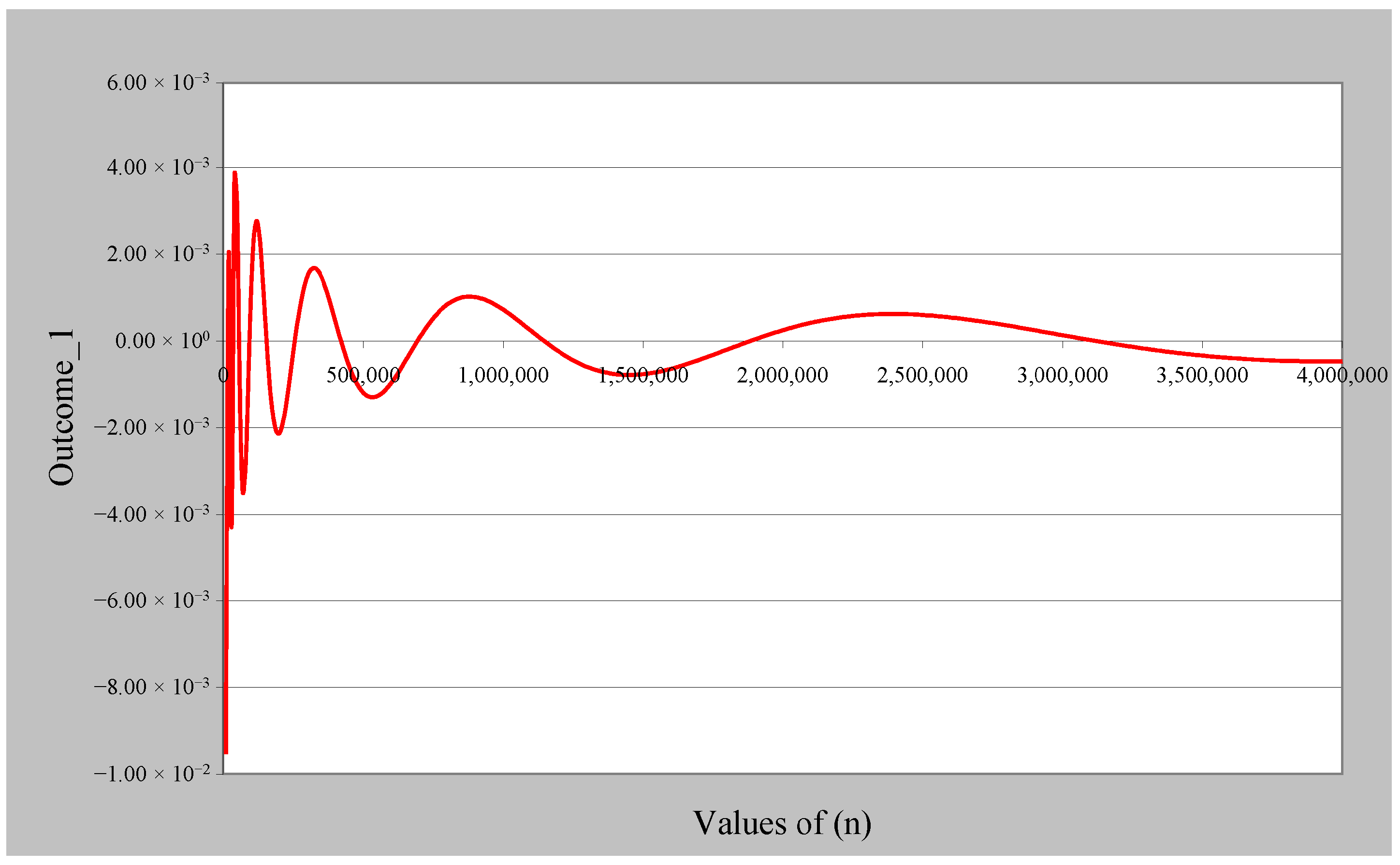
We define the quantity Outcome_1(n) by Equation (65) and evaluate it numerically for increasing values of n. Figure 3 shows the resulting values of Outcome_1(n), providing computational evidence consistent with the asymptotic result stated in Equation (28).

The decay of the oscillations is consistent with the theoretically predicted O(n^−1/2) rate derived in Remark 1. The amplitude decreases proportionally to n^−1/2, as anticipated by the asymptotic expansion.

Let us now consider Equation (29) and restate it in the following finite-n form:

$$\begin{gathered} Outcome\_2(n)={\displaystyle \frac{\frac{1}{\sqrt{1}}\sin \left((14.13\dots )\ln \frac{1}{n}+\mathrm{atan}\frac{1}{2(14.13\dots )}\right)+\frac{1}{\sqrt{2}}\sin \left((14.13\dots )\ln \frac{2}{n}+\mathrm{atan}\frac{1}{2(14.13\dots )}\right)+\dots +\frac{1}{\sqrt{n}}\sin \left((14.13\dots )\ln \frac{n}{n}+\mathrm{atan}\frac{1}{2(14.13\dots )}\right)}{\sqrt{n}}} \\ -2{\displaystyle \frac{1-4{(14.13\dots )}^2}{{(1+4{(14.13\dots )}^2)}^{3/2}}} \end{gathered}$$

(66)

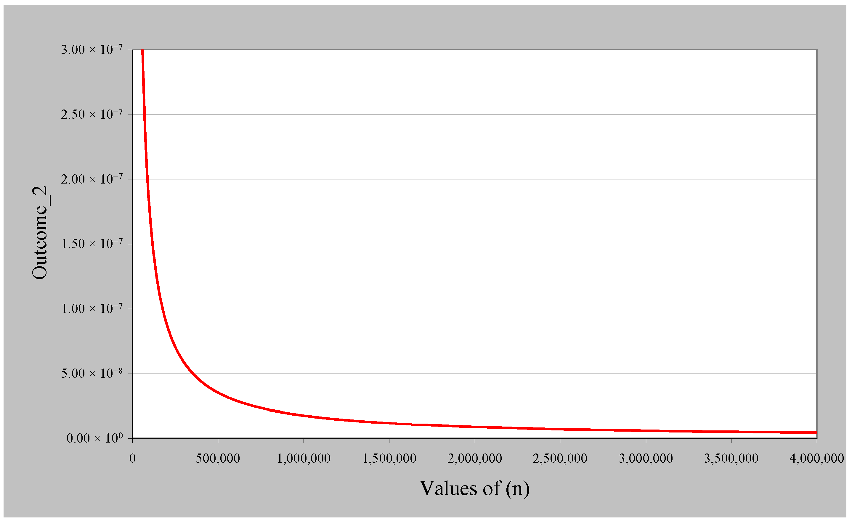
We define the quantity Outcome_2(n) by Equation (66), which is evaluated numerically for increasing values of n. Figure 4 shows the numerical evaluation of Outcome_2(n).

As observed in this case (Figure 4), where b ≈ 14.13 corresponds to a nontrivial zero of the Riemann zeta function, the decay is consistent with the O(n^−1/2) asymptotic rate, although in this case the oscillatory component is numerically suppressed. This contrasts with Figure 3 (b = 2π), where pronounced oscillations are clearly visible. Preliminary computations indicate similar behavior for additional tested values of b. This observation is consistent with the findings reported in [17], where it was shown that for generic values of b the quantity|A₂(n)|² contains a fluctuating component, whereas for values of b corresponding to nontrivial zeros of the Riemann zeta function this fluctuating component disappears. In an analogous manner, for the expression/quantity considered here (Equation (18)), an oscillatory behavior is observed for generic values of b, which vanishes when b assumes values corresponding to nontrivial zeros of the Riemann zeta function. This behavior is reasonable, as an examination of Equations (13), (61)/(62) and (18) indicates a structural link between the two quantities under consideration when b corresponds to a nontrivial zero of the Riemann zeta function.

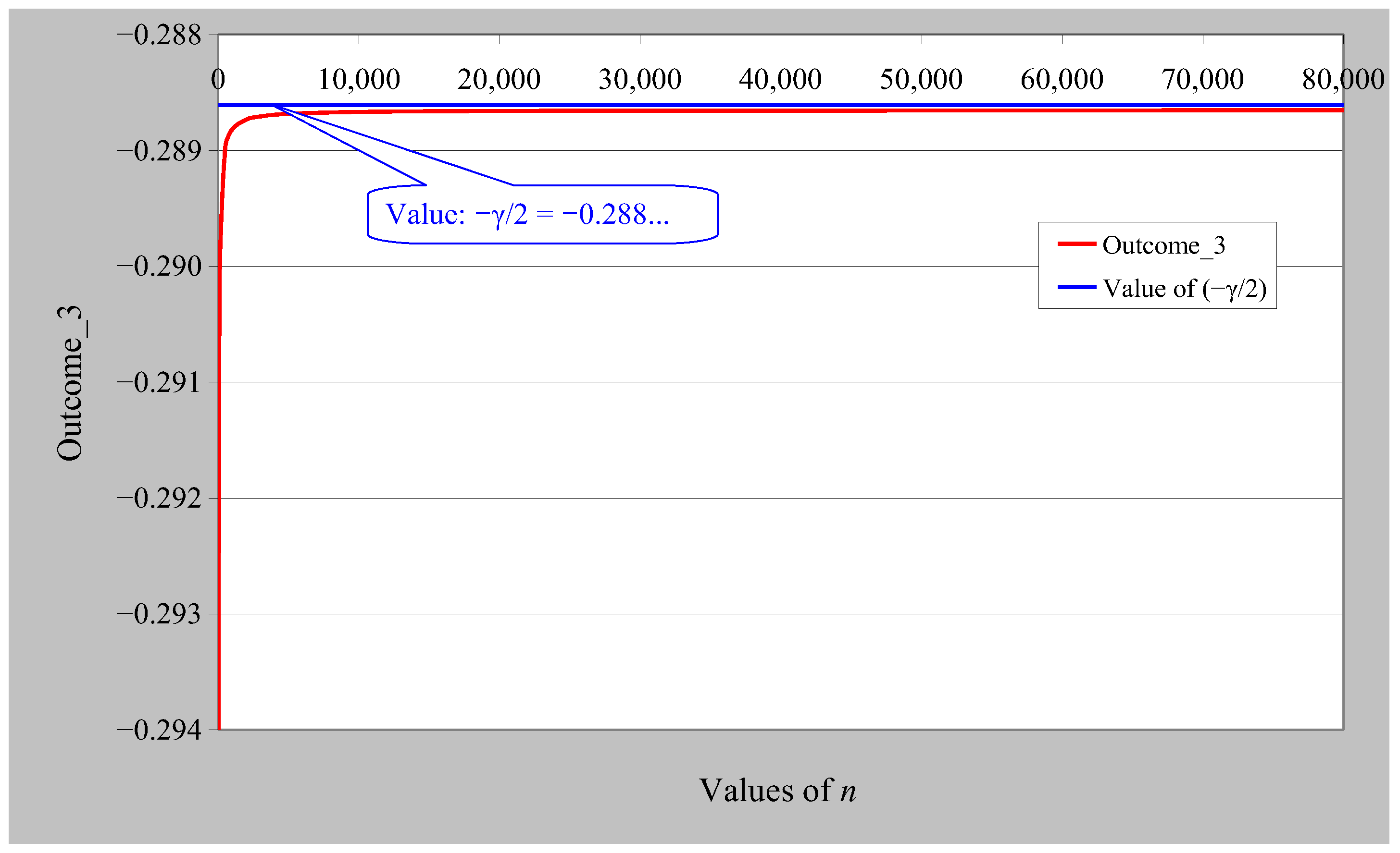
Let us further consider Equation (63) and restate it in the following finite-n form:

$$\begin{gathered} Outcome\_3(n)=\left({\displaystyle \frac{1}{\sqrt{1\cdot 2}}}\cos ((14.13\dots ) \ln {\displaystyle \frac{1}{2}})+\dots +{\displaystyle \frac{1}{\sqrt{1\cdot n}}}\cos ((14.13\dots ) \ln {\displaystyle \frac{1}{n}})+{\displaystyle \frac{1}{\sqrt{2\cdot 3}}}\cos ((14.13\dots ) \ln {\displaystyle \frac{2}{3}})+\dots +{\displaystyle \frac{1}{\sqrt{2\cdot n}}}\cos ((14.13\dots ) \ln {\displaystyle \frac{2}{n}})+\dots +{\displaystyle \frac{1}{\sqrt{(n-1)\cdot n}}}\cos ((14.13\dots ) \ln {\displaystyle \frac{(n-1)}{n}})\right) \\ -{\displaystyle \frac{\sqrt{1+4{(14.13\dots )}^2}}{1-4{(14.13\dots )}^2}}\sqrt{n}\cdot \left[{\displaystyle \frac{1}{\sqrt{1}}}\sin \left((14.13\dots )\ln {\displaystyle \frac{1}{n}}+\mathrm{atan}{\displaystyle \frac{0.5}{14.13\dots }}\right)+{\displaystyle \frac{1}{\sqrt{2}}}\sin \left((14.13\dots )\ln {\displaystyle \frac{2}{n}}+\mathrm{atan}{\displaystyle \frac{0.5}{14.13\dots }}\right)+\dots +{\displaystyle \frac{1}{\sqrt{n}}}\sin \left((14.13\dots )\ln {\displaystyle \frac{n}{n}}+\mathrm{atan}{\displaystyle \frac{0.5}{14.13\dots }}\right)\right]+{\displaystyle \frac{\ln (n)}{2}} \end{gathered}$$

(67)

We define the quantity Outcome_3(n) by Equation (67), which is evaluated numerically for increasing values of n.

As shown in Theorem 1, the first term of Equation (67) is part of the series G_tot corresponding to the n × n matrix in Figure 1. More precisely, it consists of the entries to the right of the main diagonal of this matrix; that is, it represents half of the matrix, excluding the diagonal entries. Consequently, for n = 80,000, the effective number of contributing terms is approximately 6.4 × 10⁹—a remarkably large figure. Figure 5 shows the numerical evaluation of Outcome_3(n), indicating convergence toward the theoretical value −γ/2.

Despite the extremely large number of contributing terms, the numerical evaluation remains stable and exhibits clear convergence towards the theoretical constant. This behavior is consistent with the internal coherence of the derived relations.

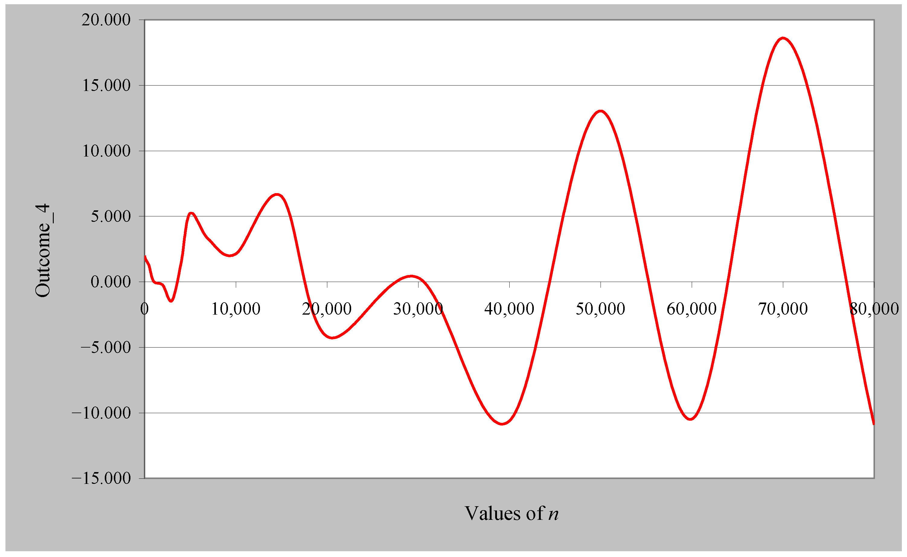
Furthermore, it is instructive to investigate the behavior of Outcome_4 when, in Equation (62), instead of selecting b corresponding to a nontrivial zero, we choose a generic value, for example b = 17. In this case, Equation (67) becomes Equation (68).

$$\begin{gathered} Outcome\_4(n)=\left({\displaystyle \frac{1}{\sqrt{1\cdot 2}}}\cos (17 \ln {\displaystyle \frac{1}{2}})+\dots +{\displaystyle \frac{1}{\sqrt{1\cdot n}}}\cos ((17 \ln {\displaystyle \frac{1}{n}})+{\displaystyle \frac{1}{\sqrt{2\cdot 3}}}\cos (17 \ln {\displaystyle \frac{2}{3}})+\dots +{\displaystyle \frac{1}{\sqrt{2\cdot n}}}\cos (17 \ln {\displaystyle \frac{2}{n}})+\dots +{\displaystyle \frac{1}{\sqrt{(n-1)\cdot n}}}\cos (17 \ln {\displaystyle \frac{(n-1)}{n}})\right) \\ -{\displaystyle \frac{\sqrt{1+4\cdot {17}^2}}{1-4\cdot {17}^2}}\sqrt{n}\cdot \left[{\displaystyle \frac{1}{\sqrt{1}}}\sin \left(17\ln {\displaystyle \frac{1}{n}}+\mathrm{atan}{\displaystyle \frac{0.5}{17}}\right)+{\displaystyle \frac{1}{\sqrt{2}}}\sin \left(17\ln {\displaystyle \frac{2}{n}}+\mathrm{atan}{\displaystyle \frac{0.5}{17}}\right)+\dots +{\displaystyle \frac{1}{\sqrt{n}}}\sin \left(17\ln {\displaystyle \frac{n}{n}}+\mathrm{atan}{\displaystyle \frac{0.5}{17}}\right)\right]+{\displaystyle \frac{\ln (n)}{2}} \end{gathered}$$

(68)

We define the quantity Outcome_4(n) by Equation (68), which is evaluated numerically for increasing values of n. Figure 6 shows the numerical evaluation of Outcome_4(n).

In this case, the quantity does not converge to (−γ/2) nor to any finite value, but instead exhibits growing oscillatory behavior. This contrasts with Figure 5, where clear convergence is observed when b corresponds to a nontrivial zero of the Riemann zeta function. The comparison highlights the structural role of the parameter b in the asymptotic cancellation mechanism.

Finally, let us consider Equation (64), and restate it in the following finite-n form:

Q(n) = Q₁(n) − Q₂(n)

(69)

where

$$\begin{gathered} Q_1(n)=\left({\displaystyle \frac{1}{\sqrt{1\cdot 2}}}\cos ((14.13\dots ) \ln {\displaystyle \frac{1}{2}})+\dots +{\displaystyle \frac{1}{\sqrt{1\cdot n}}}\cos ((14.13\dots ) n{\displaystyle \frac{1}{n}})+{\displaystyle \frac{1}{\sqrt{2\cdot 3}}}\cos ((14.13\dots )\ln {\displaystyle \frac{2}{3}})+\dots +{\displaystyle \frac{1}{\sqrt{2\cdot n}}}\cos ((14.13\dots ) \ln {\displaystyle \frac{2}{n}})+\dots +{\displaystyle \frac{1}{\sqrt{(n-1)\cdot n}}}\cos ((14.13\dots )\ln {\displaystyle \frac{(n-1)}{n}})\right) \\ -{\displaystyle \frac{\sqrt{1+{(14.13\dots )}^2}}{1-{(14.13\dots )}^2}}\sqrt{n}\cdot \left[{\displaystyle \frac{1}{1^a}}\sin \left((14.13\dots ) \ln {\displaystyle \frac{1}{n}}+\mathrm{atan}{\displaystyle \frac{0.5}{14.13\dots }}\right)+{\displaystyle \frac{1}{2^a}}\sin \left((14.13\dots ) \ln {\displaystyle \frac{2}{n}}+\mathrm{atan}{\displaystyle \frac{0.5}{14.13\dots }}\right)+\dots +{\displaystyle \frac{1}{n^a}}\sin \left((14.13\dots ) \ln {\displaystyle \frac{n}{n}}+\mathrm{atan}{\displaystyle \frac{0.5}{14.13\dots }}\right)\right] \end{gathered}$$

and

$$\begin{gathered} Q_2(n)=\left({\displaystyle \frac{1}{\sqrt{1\cdot 2}}}\cos ((49.77\dots ) \ln {\displaystyle \frac{1}{2}})+\dots +{\displaystyle \frac{1}{\sqrt{1\cdot n}}}\cos ((49.77\dots ) n{\displaystyle \frac{1}{n}})+{\displaystyle \frac{1}{\sqrt{2\cdot 3}}}\cos (((49.77\dots )\ln {\displaystyle \frac{2}{3}})+\dots +{\displaystyle \frac{1}{\sqrt{2\cdot n}}}\cos ((49.77\dots ) \ln {\displaystyle \frac{2}{n}})+\dots +{\displaystyle \frac{1}{\sqrt{(n-1)\cdot n}}}\cos ((49.77\dots )\ln {\displaystyle \frac{(n-1)}{n}})\right) \\ -{\displaystyle \frac{\sqrt{1+{(49.77\dots )}^2}}{1-{(49.77\dots )}^2}}\sqrt{n}\cdot \left[{\displaystyle \frac{1}{1^a}}\sin \left((49.77\dots ) \ln {\displaystyle \frac{1}{n}}+\mathrm{atan}{\displaystyle \frac{0.5}{49.77\dots }}\right)+{\displaystyle \frac{1}{2^a}}\sin \left((49.77\dots ) \ln {\displaystyle \frac{2}{n}}+\mathrm{atan}{\displaystyle \frac{0.5}{49.77\dots }}\right)+\dots +{\displaystyle \frac{1}{n^a}}\sin \left((49.77\dots ) \ln {\displaystyle \frac{n}{n}}+\mathrm{atan}{\displaystyle \frac{0.5}{49.77\dots }}\right)\right] \end{gathered}$$

Using computer code once again, we can compute the difference Q = Q1 − Q2 for n = 3000, yielding Q(3000) ≈ −8.62 × 10⁻⁴ a value that is already very close to zero, which is consistent with Equation (64). The magnitude of Q(n) decreases as n increases, in accordance with the cancellation mechanism suggested by the theoretical analysis.

The computational experiments presented above are consistent with the theoretical asymptotic analysis. For generic parameter values b, the expressions exhibit oscillatory or unstable growth, whereas for values of b corresponding to nontrivial zeros of the Riemann zeta function, a cancellation mechanism is observed. This cancellation is associated with either algebraic decay or convergence toward the predicted constant −γ/2, depending on the structure of the corresponding relation. The contrast between the two regimes highlights the structural role of the parameter b in the asymptotic behavior of the derived expressions.

Although numerical evidence does not constitute a proof, the large-scale computations performed in double-precision arithmetic provide consistency checks for the internal coherence of the representative asymptotic framework. The numerical experiments are intended solely as supportive consistency tests of the formal asymptotic predictions and do not constitute independent analytical justification.

5. Conclusions

The Riemann zeta function ζ(s), since its analytic continuation by Riemann and the establishment of its functional equation, has remained a central object of investigation in analytic number theory. The structural properties of its nontrivial zeros, particularly on the critical line, continue to motivate the development of alternative analytical perspectives.

In the present work, we examined a class of asymptotic relations involving series associated with ζ(s) within the formal infinite number representative framework introduced in Section 2. By constructing an n × n matrix and analyzing the associated expressions in the asymptotic regime n → ∞, we derived a family of structured relations connecting matrix-defined sums with Dirichlet-type expressions on the critical line.

Within this representative setting, the analysis shows that when the parameter b coincides with the imaginary part of a nontrivial zero of the Riemann zeta function, a systematic cancellation mechanism emerges. This leads to parameter-dependent asymptotic behavior, including algebraic decay or convergence toward the constant −γ/2, depending on the structure of the expression considered. These relations are obtained consistently within the representative framework and are supported by numerical computations that confirm the predicted asymptotic behavior.

The contribution of the present work is therefore methodological: it introduces a coherent representative asymptotic calculus through which divergent and oscillatory expressions may be organized and compared in a structured manner. Within this framework, identities are interpreted at the level of asymptotic representatives, allowing consistent manipulation of expressions that fall outside the scope of classical convergence.

The proposed approach does not modify the classical analytic continuation of ζ(s) nor does it aim to replace established methods of analytic number theory. Rather, it provides an alternative structural perspective that complements standard techniques by highlighting asymptotic relationships that are not immediately accessible through classical formulations.

Under this interpretation, the present study may be viewed as a systematic asymptotic framework for organizing identities involving divergent expressions associated with the Riemann zeta function. The consistency of the derived relations, together with their numerical validation, indicates that the representative approach captures meaningful structural features of the underlying analytic objects.

An interesting direction for future research is the further structural development of the representative asymptotic framework introduced here, in particular through a more systematic formulation of equivalence classes of asymptotic behaviors and their associated algebraic properties. Such an extension may provide a deeper connection between the present formalism and established asymptotic or functional–analytic structures.