Parameter Estimation for the Linear Self-Attracting Diffusion Processes

Abstract

In this paper, we investigate parameter estimation for a class of linear self-attracting diffusion processes. Specifically, we consider processes with a drift coefficient given by $-\theta \left({\int }_0^t(X_t-X_u)du\right)$. Employing both maximum likelihood estimation and least squares estimation, we show that the resulting estimators coincide. We establish the consistency and asymptotic normality of ${\widehat{\theta }}_N$ for high-frequency data, and assess its numerical performance through simulation studies.

1. Introduction

In 1995, Cranston and Le Jan [1] introduced a linear self-attracting diffusion process. This process satisfies a stochastic differential equation (SDE) of the following form:

$$\left\{\begin{array}{c}d{X}_t=d{B}_t-\theta \left({\int }_0^t(X_t-X_u)du\right)dt,\hfill \\ X_0=0.\hfill \end{array}\right.$$

(1)

where the parameter $\theta >0$ is a constant. The solution to this equation was shown to be unique. As a result, $X_t$ converges both in mean square and almost surely to a normally distributed random variable. Equation (1) is a special case of self-interacting diffusion invented by Durrett and Rogers [2] in 1992. The processes have been studied from different aspects for many years. Herrmann and Michael [3] analyze the rate of convergence for certain self-attracting diffusions and establish an estimate specifically for the linear case. Yan et al. [4] introduce a linear fractional self-attracting diffusion. This process is driven by a fractional Brownian motion with Hurst index ${\displaystyle \frac{1}{2}}<H<1$. They study its convergence and the corresponding weighted local time. Jie He and Qian Guo [5] propose an explicit numerical scheme to approximate the linear self-interacting diffusion. They analyze the mean-square convergence of this method and establish that its convergence order is 1. Prior research is predicated on the assumption that the parameter $\theta$ is known. Given that $\theta$ is inherently unknown in practical applications, its estimation is therefore essential.

As a core branch of statistical inference, parameter estimation plays an irreplaceable role. In the statistical applications of SDEs, parameter estimation has accumulated a substantial body of systematic research findings [6]. These findings include weak consistency [7], strong consistency [8], and asymptotic normality [9], all of which have been extensively studied. Yan et al. [10] investigate the asymptotic properties of the least squares estimators under continuous observation. They establish the strong consistency and asymptotic normality of the estimators. Jørgensen and Sørensen [11] proved the existence of a consistent estimator under the conditions ${\Delta }_n\to 0$ and $n{\Delta }_n\to \infty$. They further established the asymptotic normality of the estimator under the additional rate condition $n{\Delta }_n^3\to 0$. Mazzonetto and Nieto [12] proved the consistency and asymptotic normality of MLE and quasi-maximum likelihood estimators for the drift parameters of ergodic threshold Chan–Karolyi–Longstaff–Sanders processes. Their results apply to both continuous observations and high-frequency discrete observations with an infinite horizon.

Stochastic process observation schemes are divided into continuous and discrete types. Continuous observation of diffusion represents a mathematical idealization, underpinned by a robust theoretical framework. However, as practical measurement equipment cannot realize continuous tracking, real-world observational data are inherently discrete. In light of this, this paper derives the maximum likelihood estimator (MLE) and least squares estimator (LSE) for the parameter $\theta$ under continuous and discrete observation scenarios, respectively.

We now clarify the relationship between our approach and the works of Han [13] and Chen et al. [14]. Under the discrete observation framework, both prior works explicitly employ the auxiliary process $Z_t={\int }_0^t(X_t-X_u)du$ to construct their estimators and derive corresponding theoretical properties. Nevertheless, the process $Z_t$ itself is unobservable in practice, as only discrete measurements $X_{t_1},X_{t_2},\dots ,X_{t_N}$ are accessible in real applications. To overcome this critical limitation, we propose a discrete-time approximation ${\widehat{Z}}_{t_i}=h{\displaystyle \sum _{j=0}^{i-1}}(X_{t_i}-X_{t_j})$ for the unobservable $Z_t$ in this paper.

The structure of the paper is as follows. In the next section, we introduce an auxiliary process $Z_t={\int }_0^t(X_t-X_u)du$. With this process, we rewrite the SDE (1) as a two-dimensional vector SDE (4). In Section 3, we derive MLE and LSE for both continuous and discrete observations. In Section 4, we focus on the continuous observation framework. As $T\to \infty$, we prove the almost sure convergence of ${\widehat{\theta }}_T$ to ${\theta }_0$ and establish a central limit theorem. In Section 5, we consider the discrete observation framework. Under the conditions $T\to \infty$ and $T^2/N\to 0$, we establish the convergence in probability of ${\widehat{\theta }}_N$ to ${\theta }_0$. Finally, in Section 6, we examine the finite-sample performance of ${\widehat{\theta }}_N$ with simulated data. Numerical results are shown.

2. Preliminaries

In the theory of ordinary differential equations [15], it is a well-established result that higher-order ordinary differential equations can be reformulated as systems of first-order ordinary differential equations. This approach not only greatly reduces the analytical complexity of such equations but also provides a convenient framework for their numerical solution. In a similar spirit, we introduce an auxiliary stochastic process defined by $Z_t={\int }_0^t(X_t-X_u)du$. The Itô formula gives

$$\begin{array}{cc}\hfill d{Z}_t& =d\left(t{X}_t\right)-X_{t}dt=X_{t}dt+td{X}_t-X_{t}dt=-\theta t{Z}_{t}dt+td{B}_t,\hfill \end{array}$$

then $Z_t$ satisfies a linear SDE. Considering the integrating factor [16] $e^{{\displaystyle \frac{\theta t^2}{2}}}$, then

$$d(e^{{\displaystyle \frac{\theta t^2}{2}}}{Z}_t)=\theta t{e}^{{\displaystyle \frac{\theta t^2}{2}}}{Z}_{t}dt+e^{{\displaystyle \frac{\theta t^2}{2}}}d{Z}_t=t{e}^{{\displaystyle \frac{\theta t^2}{2}}}d{B}_t,$$

which yields

$$Z_t=e^{-{\displaystyle \frac{\theta t^2}{2}}}{\int }_0^{t}s{e}^{{\displaystyle \frac{\theta s^2}{2}}}d{B}_s,$$

(2)

and

$$X_t={\int }_0^t\left(1-\theta s{e}^{{\displaystyle \frac{\theta s^2}{2}}}{\int }_s^t{e}^{-{\displaystyle \frac{\theta u^2}{2}}}du\right)d{B}_s.$$

(3)

Building on the formulation $d{Z}_t=-\theta t{Z}_{t}dt+td{B}_t$, we define the state components as $Y_{1,t}=X_t$ and $Y_{2,t}=Z_t$. This allows us to rewrite the SDE (1) as a two-dimensional vector SDE.

$$d{Y}_t=\left(\begin{array}{cc}0& -\theta \\ 0& -t\theta \end{array}\right)Y_{t}dt+\left(\begin{array}{c}1\\ t\end{array}\right)d{B}_t,Y_0=\left(\begin{array}{c}0\\ 0\end{array}\right).$$

(4)

where

$$a(t,Y_t)=\left(\begin{array}{cc}0& -\theta \\ 0& -t\theta \end{array}\right)Y_t=\left(\begin{array}{c}-\theta Y_{2,t}\\ -t\theta Y_{2,t}\end{array}\right),b(t,Y_t)=\left(\begin{array}{c}1\\ t\end{array}\right).$$

Note that the linear self-attracting diffusion $\{X_t,t\ge 0\}$ does not have the Markov property. However, after introducing the auxiliary stochastic process $Z_t$, the bivariate stochastic process $\{(X_t,Z_t),t\ge 0\}$ is a two-dimensional Markov process.

Given that the coefficients $a(t,Y_t)$ and $b(t,Y_t)$ satisfy the global Lipschitz and linear growth conditions, the well-known Euler–Maruyama method [17] can be used to obtain numerical solutions. For two-dimensional vector SDE (4), the Euler–Maruyama scheme is given:

$$Y^{n+1}=Y^n+a(t_n,Y^n)h+b(t_n,Y^n)\Delta B_n,$$

where $\Delta B_n=B_{t_{n+1}}-B_{t_n}$. The discrete time approximation $Y^n$ converges strongly to the exact solution $Y_{t_n}$ with order $\gamma =0.5$. In particular, under the additive noise $b(t,Y_t)={\left(\begin{array}{cc}1& t\end{array}\right)}^T$, it turns out that the Euler–Maruyama scheme has order of strong convergence $\gamma =1$. Thus,

$$\mathbb{E}\left(\left|X_T-Y_1^N\right|\right)\le \mathbb{E}\left(\sqrt{{\left(X_T-Y_1^N\right)}^2+{\left(Z_T-Y_2^N\right)}^2}\right)=\mathbb{E}\left(\left|Y_T-Y^N\right|\right)\le C·h.$$

The analytical solution (3) is in integral form. Given the complex dependence with respect to s, the Itô integral requires numerical approximation. Therefore, in Section 6, we employ the Euler–Maruyama method to simulate discrete observations of the linear self-attracting diffusion process $\{X_t,t\ge 0\}$.

3. Maximum Likelihood Estimator and Least Squares Estimator

Maximum likelihood and least squares are the two most commonly used methods in modern statistical inference. In this section, based on both continuous and discrete observation data, we present MLE and LSE for parameter $\theta$. The final results show that the estimators obtained by the two methods are identical.

3.1. MLE and LSE Under Continuous Observation

Let ${\mathbb{P}}_{\theta }$ be the probability measure generated by the process $\{X_t,0\le t\le T\}$ on the space $(C_T,{\mathcal{B}}_T)$, where $C_T$ denotes the set of all continuous functions from $[0,T]\to \mathbb{R}$, and ${\mathcal{B}}_T$ is the corresponding Borel $\sigma$-algebra under the supremum norm. Let ${\theta }_0$ be the true value of the parameter, which lies inside the parameter space $\Theta$, where $\Theta$ is a compact in ${\mathbb{R}}^{+}$. From (2), $Z_t$ is a zero-mean Gaussian process. Then

$${\mathbb{E}}_{{\mathbb{P}}_{{\theta }_0}}\left[exp\left\{{\displaystyle \frac{{(\theta -{\theta }_0)}^2}{2}}{\int }_0^T{Z}_t^{2}dt\right\}\right]<\infty .$$

Then, the stochastic exponential process $\left\{exp\left\{-{\int }_0^T(\theta -{\theta }_0)Z_{t}d{B}_t-{\displaystyle \frac{{(\theta -{\theta }_0)}^2}{2}}{\int }_0^T{Z}_t^{2}dt\right\},t>0\right\}$ is a martingale. According to the Girsanov theorem [18], the likelihood function can be expressed as

$$L_T\left(\theta \right):={\displaystyle \frac{d{\mathbb{P}}_{\theta }}{d{\mathbb{P}}_{{\theta }_0}}}=exp\left\{-{\int }_0^T(\theta -{\theta }_0)Z_{t}d{X}_t-{\displaystyle \frac{{\theta }^2-{\theta }_0^2}{2}}{\int }_0^T{Z}_t^{2}dt\right\}.$$

(5)

Let $l_T\left(\theta \right):=log{L}_T\left(\theta \right)$, MLE is defined as

$$\widehat{\theta }:=arg\underset{\theta \in \Theta }{sup}{l}_T\left(\theta \right).$$

By differentiating the log-likelihood function, we obtain

$${\displaystyle \frac{d{l}_T\left(\theta \right)}{d\theta }}=-{\int }_0^T{Z}_{t}d{X}_t-\theta {\int }_0^T{Z}_t^{2}dt,$$

and

$${\displaystyle \frac{d^2{l}_T\left(\theta \right)}{d{\theta }^2}}=-{\int }_0^T{Z}_t^{2}dt<0.$$

Thus, the MLE of $\theta$ is

$${\widehat{\theta }}_T=-{\displaystyle \frac{{\int }_0^T{Z}_{t}d{X}_t}{{\int }_0^T{Z}_t^{2}dt}}.$$

It should be noted that the self-attracting diffusion process considered in this paper requires $\theta >0$. Strictly speaking, ${\widehat{\theta }}_T$ is not the MLE of $\theta$, as it may take negative values. A rigorous definition is provided in Kutoyants [19]. Nevertheless, we retain this terminology for convenience.

In order to obtain LSE under continuous observation data, following the approach of Hu and Nualart [20], we consider the following objective function:

$$S_T\left(\theta \right)={\int }_0^T{\left|{\dot{X}}_t-(-\theta Z_t)\right|}^{2}dt.$$

The notation ${\dot{X}}_t$ is a widely used convention in physics and applied stochastic analysis. As the underlying process $\{X_t,t\ge 0\}$ is an Itô process driven by Brownian motion—its sample paths being almost nowhere differentiable—the symbol ${\dot{X}}_t$ is not mathematically well-defined in the classical sense. It is instead employed as a formal shorthand, with the intended meaning that ${\dot{X}}_{t}dt=d{X}_t$. LSE for $\theta$ is then defined as

$$\widehat{\theta }:=arg\underset{\theta \in \Theta }{inf}{S}_T\left(\theta \right).$$

Differentiating the objective function yields

$${\displaystyle \frac{d{S}_T\left(\theta \right)}{d\theta }}=2{\int }_0^T\left({\dot{X}}_t+\theta Z_t\right)Z_{t}dt=2{\int }_0^T{Z}_{t}d{X}_t+2\theta {\int }_0^T{Z}_t^{2}dt,$$

and

$${\displaystyle \frac{d^2{S}_T\left(\theta \right)}{d{\theta }^2}}=2{\int }_0^T{Z}_t^{2}dt>0.$$

Thus, LSE of $\theta$ is

$${\widehat{\theta }}_T=-{\displaystyle \frac{{\int }_0^T{Z}_{t}d{X}_t}{{\int }_0^T{Z}_t^{2}dt}},$$

which is identical to MLE. Therefore, the same notation is used.

3.2. MLE and LSE Under Discrete Observation

In the preceding subsection, we focused on the setting where the self-attracting diffusion process is observed continuously. In practice, however, it is difficult to obtain fully continuous observations of the sample path, and discrete sampling is far more common. Thus, we consider high-frequency observations of the self-attracting diffusion process $\{X_t,t\ge 0\}$ over an infinite time horizon. Specifically, observations are made at equally spaced discrete time points $t_0,t_1,t_2,\dots ,t_N$, i.e., $t_i=ih$, so that $Nh=T$. We assume that ${\displaystyle \frac{T^2}{N}}\to 0$ as $N\to \infty$. This condition has two important implications. First, it ensures that the total observation time $T=Nh$ tends to infinity, which is necessary for obtaining consistent estimates of parameter $\theta$. Second, it reflects the high-frequency nature of the observations, enabling us to better approximate the continuous-time process by discrete-time data.

Parameter estimation for general diffusion processes follows two common approaches. The first approach constructs the MLE from continuous observations and then approximates it using discrete samples. The second approach directly formulates the MLE or LSE from discrete observations by leveraging a discretized version of the diffusion process. In the context of discrete observations, this paper adopts the first approach to construct the MLE. Following the method of Yoshida [21], we approximate the likelihood function in Equation (5) to derive the approximate log-likelihood function:

$$\begin{array}{c}\hfill l_N\left(\theta \right)=\sum _{i=0}^{N-1}\left[(-\theta {\widehat{Z}}_{t_i})+{\theta }_0{\widehat{Z}}_{t_i}\right](X_{t_{i+1}}-X_{t_i})-{\displaystyle \frac{1}{2}}\sum _{i=0}^{N-1}\left[{(-\theta {\widehat{Z}}_{t_i})}^2-{(-{\theta }_0{\widehat{Z}}_{t_i})}^2\right](t_{i+1}-t_i).\end{array}$$

It is important to note here that our observation data are $X_{t_0},X_{t_1},\dots ,X_{t_N}$. The auxiliary stochastic process $\{Z_t,t\ge 0\}$ is unobservable, and therefore needs to be estimated using the observable data. Specifically, an estimator for $Z_{t_i}$ can be constructed as: ${\widehat{Z}}_{t_i}=h{\displaystyle \sum _{j=0}^{i-1}}(X_{t_i}-X_{t_j})$. Differentiating the aforementioned approximate log-likelihood function yields

$${\displaystyle \frac{d{l}_N\left(\theta \right)}{d\theta }}=-\sum _{i=0}^{N-1}{\widehat{Z}}_{t_i}(X_{t_{i+1}}-X_{t_i})-\theta \sum _{i=0}^{N-1}{\widehat{Z}}_{t_i}^2(t_{i+1}-t_i),$$

and

$${\displaystyle \frac{d^2{l}_N\left(\theta \right)}{d{\theta }^2}}=-\sum _{i=0}^{N-1}{\widehat{Z}}_{t_i}^2(t_{i+1}-t_i)<0.$$

Thus, the approximate MLE of $\theta$ is

$${\widehat{\theta }}_N=-{\displaystyle \frac{{\displaystyle \sum _{i=0}^{N-1}{\widehat{Z}}_{t_i}(X_{t_{i+1}}-X_{t_i})}}{{\displaystyle h\sum _{i=0}^{N-1}{\widehat{Z}}_{t_i}^2}}},$$

where ${\widehat{Z}}_{t_i}=h{\displaystyle \sum _{j=0}^{i-1}}(X_{t_i}-X_{t_j})$.

To obtain LSE based on discrete observations, we consider the Euler–Maruyama method. This approach is motivated by Florens–Zmirou [22], who studied a minimum contrast estimator based on a first-order Euler–Maruyama type discrete time approximation of the SDE. Therefore, the first step is to construct the Euler–Maruyama scheme for Equation (1). The Euler–Maruyama scheme for Equation (1) is given by

$$X_{t_{i+1}}-X_{t_i}=-\theta h{\widehat{Z}}_{t_i}+\Delta B_{t_i},$$

where $\Delta B_{t_i}=B_{t_{i+1}}-B_{t_i}\sim N(0,h)$ and ${\widehat{Z}}_{t_i}=h{\displaystyle \sum _{j=0}^{i-1}}(X_{t_i}-X_{t_j})$. Treating $X_{t_{i+1}}-X_{t_i}$ as the dependent variable, $h{\widehat{Z}}_{ti}$ as the independent variable, and $\Delta B_{t_{i+1}}$ as the random error term, the parameter $\theta$ becomes the unknown coefficient in the regression equation. According to the classical least squares method, the objective function in this case is

$$S_N\left(\theta \right)=\sum _{i=0}^{N-1}{\left|X_{t_{i+1}}-X_{t_i}-(-\theta h{\widehat{Z}}_{t_i})\right|}^2.$$

Differentiating the objective function yields

$${\displaystyle \frac{d{S}_N\left(\theta \right)}{d\theta }}=2h\sum _{i=0}^{N-1}\left(X_{t_{i+1}}-X_{t_i}+\theta h{\widehat{Z}}_{t_i}\right){\widehat{Z}}_{t_i},$$

and

$${\displaystyle \frac{d^2{S}_N\left(\theta \right)}{d{\theta }^2}}=2h^2\sum _{i=0}^{N-1}{\widehat{Z}}_{t_i}^2>0.$$

Thus, LSE of $\theta$ is

$${\widehat{\theta }}_N=-{\displaystyle \frac{{\displaystyle \sum _{i=0}^{N-1}{\widehat{Z}}_{t_i}(X_{t_{i+1}}-X_{t_i})}}{{\displaystyle h\sum _{i=0}^{N-1}{\widehat{Z}}_{t_i}^2}}},$$

which is identical to the approximate MLE. Therefore, the same notation is used.

The results above indicate that, whether under continuous or discrete observations, the expressions for MLE and LSE are identical. Therefore, hereafter, we will collectively refer to them as the estimator, without further emphasis on which specific estimation method is employed.

4. Asymptotic Properties of the Estimator ${\widehat{\mathit{\theta }}}_{\mathit{T}}$ Under Continuous Observation

The asymptotic properties of a parameter estimator provide an intuitive reflection of the estimator’s effectiveness and the corresponding estimation method, thereby offering solid theoretical support for the rationality and reliability of the method. Without such asymptotic theoretical guarantees, any statistical inference based on finite samples would lack scientific justification. For this reason, this chapter focuses on studying the consistency and asymptotic normality of the proposed estimator.

Consistency is the most fundamental and essential requirement for any reasonable point estimator [23]. The following theorem shows that the estimator ${\widehat{\theta }}_T$ is a strongly consistent estimator of ${\theta }_0$.

Theorem 1.

There exists a root ${\widehat{\theta }}_T$ to $l_T^{\prime }\left(\theta \right)=0$, which is strongly consistent, i.e.,

$${\mathbb{P}}_{{\theta }_0}\left(\underset{T\to \infty }{lim}{\widehat{\theta }}_T={\theta }_0\right)=1.$$

Proof. 

Observe that, for $\forall \delta >0$,

$$\begin{array}{cc}\hfill l_T\left({\theta }_0\right)-l_T({\theta }_0+\delta )& =\delta {\int }_0^T{Z}_{t}d{X}_t+{\displaystyle \frac{2\delta {\theta }_0+{\delta }^2}{2}}{\int }_0^T{Z}_t^{2}dt\hfill \\ \hfill & =\delta {\int }_0^T{Z}_{t}d{B}_t-\delta {\theta }_0{\int }_0^T{Z}_t^{2}dt+{\displaystyle \frac{2\delta {\theta }_0+{\delta }^2}{2}}{\int }_0^T{Z}_t^{2}dt\hfill \\ \hfill & =\delta {\int }_0^T{Z}_{t}d{B}_t+{\displaystyle \frac{{\delta }^2}{2}}{\int }_0^T{Z}_t^{2}dt.\hfill \end{array}$$

Then

$${\displaystyle \frac{l_T\left({\theta }_0\right)-l_T({\theta }_0+\delta )}{{\delta }^2{\int }_0^T{Z}_t^{2}dt}}={\displaystyle \frac{1}{\delta }}{\displaystyle \frac{{\int }_0^T{Z}_{t}d{B}_t}{{\int }_0^T{Z}_t^{2}dt}}+{\displaystyle \frac{1}{2}}.$$

Similarly, we obtain

$${\displaystyle \frac{l_T\left({\theta }_0\right)-l_T({\theta }_0-\delta )}{{\delta }^2{\int }_0^T{Z}_t^{2}dt}}=-{\displaystyle \frac{1}{\delta }}{\displaystyle \frac{{\int }_0^T{Z}_{t}d{B}_t}{{\int }_0^T{Z}_t^{2}dt}}+{\displaystyle \frac{1}{2}}.$$

From (2), it follows that for any $0<T<\infty$,

$$\mathbb{P}\left(0<{\int }_0^T{Z}_t^{2}dt<\infty \right)=1,$$

and

$$\mathbb{P}\left({\int }_0^{\infty }{Z}_t^{2}dt=\infty \right)=1.$$

Using the strong law of large numbers for Brownian motion [24],

$$\underset{T\to \infty }{lim}{\displaystyle \frac{{\int }_0^T{Z}_{t}d{B}_t}{{\int }_0^T{Z}_t^{2}dt}}=0,a.s.$$

Therefore, for almost every $\omega \in \mathrm{\Omega }$, there exist some $T_0>0$ such that for $T\ge T_0$,

$$l_T\left({\theta }_0\right)>l_T({\theta }_0\pm \delta ).$$

Since $l_T\left(\theta \right)$ is continuous in $\theta$ on the compact set $[{\theta }_0-\delta ,{\theta }_0+\delta ]$, it has a local maximum and it is attained at a measurable $\widehat{\theta }$ in $[{\theta }_0-\delta ,{\theta }_0+\delta ]$. Since $l_T\left({\theta }_0\right)>l_T({\theta }_0\pm \delta )$, for almost every $\omega \in \mathrm{\Omega }$, there exist some $T_0>0$ such that for $T\ge T_0$, $\widehat{\theta }\in ({\theta }_0-\delta ,{\theta }_0+\delta )$. i.e.,

$${\mathbb{P}}_{{\theta }_0}\left(\underset{T\to \infty }{lim}\widehat{\theta }={\theta }_0\right)=1.$$

Since $l_T\left(\theta \right)$ is differentiable with respect to $\theta$, it follows that $l_T^{\prime }\left(\widehat{\theta }\right)=0$. From the derivation of ${\widehat{\theta }}_T$, we have ${\widehat{\theta }}_T=\widehat{\theta }$. Consequently, the estimator ${\widehat{\theta }}_T$ is a strongly consistent estimator of the true value ${\theta }_0$. □

Theorem 2.

${\widehat{\theta }}_T$ is asymptotically normally distributed. As $T\to \infty$,

$${\left({\int }_0^T{Z}_t^{2}dt\right)}^{1/2}({\widehat{\theta }}_T-{\theta }_0)\stackrel{\mathcal{D}}{⟶}N(0,1).$$

Proof. 

$${\widehat{\theta }}_T=-{\displaystyle \frac{{\int }_0^T{Z}_{t}d{X}_t}{{\int }_0^T{Z}_t^{2}dt}}=-{\displaystyle \frac{-{\theta }_0{\int }_0^T{Z}_t^{2}dt+{\int }_0^T{Z}_{t}d{B}_t}{{\int }_0^T{Z}_t^{2}dt}}={\theta }_0-{\displaystyle \frac{{\int }_0^T{Z}_{t}d{B}_t}{{\int }_0^T{Z}_t^{2}dt}}.$$

Then

$${\widehat{\theta }}_T-{\theta }_0=-{\displaystyle \frac{{\int }_0^T{Z}_{t}d{B}_t}{{\int }_0^T{Z}_t^{2}dt}}.$$

Since (2) holds, the process ${\int }_0^t{Z}_{s}d{B}_s$ is adapted to the natural filtration $\left\{{\mathcal{F}}_t,t\ge 0\right\}$ generated by the Brownian motion $\{B_t,t\ge 0\}$. For any $T>0$, Itô isometry implies that

$$\begin{array}{cc}\hfill \mathbb{E}\left[{\left({\int }_0^T{Z}_{t}d{B}_t\right)}^2\right]& =\mathbb{E}\left[{\int }_0^T{Z}_t^{2}dt\right]\hfill \\ \hfill & ={\int }_0^T{e}^{-\theta t^2}\mathbb{E}\left[{\int }_0^t{s}^2{e}^{\theta s^2}ds\right]dt\hfill \\ \hfill & \le {\int }_0^T{e}^{-\theta t^2}{e}^{\theta t^2}{\int }_0^t{s}^{2}dsdt<\infty .\hfill \end{array}$$

Therefore, ${\int }_0^T{Z}_{t}d{B}_t$ is a square-integrable martingale, with $\mathbb{E}\left[{\int }_0^T{Z}_{t}d{B}_t\right]=0$ and its quadratic variation being ${\int }_0^T{Z}_t^{2}dt$. Consequently, by the central limit theorem for square-integrable martingales [25], it follows that as $T\to \infty$,

$${\displaystyle \frac{{\int }_0^T{Z}_{t}d{B}_t}{\sqrt{{\int }_0^T{Z}_t^{2}dt}}}\stackrel{\mathcal{D}}{⟶}N(0,1).$$

Then

$${\left({\int }_0^T{Z}_t^{2}dt\right)}^{1/2}({\widehat{\theta }}_T-{\theta }_0)\stackrel{\mathcal{D}}{⟶}N(0,1).$$

The desired conclusion is established. □

5. Asymptotic Properties of the Estimator ${\widehat{\mathit{\theta }}}_{\mathit{N}}$ Under Discrete Observation

It is well known that the theory of diffusion processes is established on the basis of continuous-time observations, and many of their important properties also rely on the continuity of time. Therefore, when conducting statistical inference for diffusion processes under continuous observation, there are many well-developed tools available, which makes the statistical inference problem relatively tractable in such a scenario. However, in practical situations with discrete observations, many tools suitable for continuous observation are difficult to apply directly, thereby making the statistical inference problem for diffusion processes based on discrete observational data more challenging.

Before formally establishing the weak consistency and asymptotic normality of the estimator ${\widehat{\theta }}_N$, we introduce several key lemmas. For a fixed T, these lemmas establish the convergence rate of the numerator and denominator of ${\widehat{\theta }}_N$ to the corresponding terms in ${\widehat{\theta }}_T$. This convergence occurs in mean square and quantifies the information loss induced by discretization.

Lemma 1.

For all $s,t\in [0,T]$, the solution $X_t$ satisfies

$$\mathbb{E}|X_t-X_s{|}^2\le C|t-s|.$$

where here, and in the following, C denotes a universal positive constant, which is independent of T and N, and whose value may change from line to line.

Proof. 

Without loss of generality, assume $0\le s\le t\le T$. First, we determine the range of $h(t,s)$. Since $\theta >0$ and $0\le s\le t$, we have $h(t,s)=1-\theta s{e}^{{\displaystyle \frac{\theta s^2}{2}}}{\int }_s^t{e}^{-{\displaystyle \frac{\theta u^2}{2}}}du\le 1$.

$$\begin{array}{cc}\hfill h(t,s)& \ge 1-e^{{\displaystyle \frac{\theta s^2}{2}}}{\int }_s^t\theta u{e}^{-{\displaystyle \frac{\theta u^2}{2}}}du\hfill \\ \hfill & =1+e^{{\displaystyle \frac{\theta s^2}{2}}}\left(e^{-{\displaystyle \frac{\theta t^2}{2}}}-e^{-{\displaystyle \frac{\theta s^2}{2}}}\right)\hfill \\ \hfill & =e^{-{\displaystyle \frac{\theta (t^2-s^2)}{2}}}>0.\hfill \end{array}$$

Then, using the independence of the random variables ${\int }_0^s\left(h(t,r)-h(s,r)\right)d{B}_r$ and ${\int }_s^{t}h(t,r)d{B}_r$, along with the Itô isometry, we obtain

$$\begin{array}{cc}\hfill \mathbb{E}{\left|X_t-X_s\right|}^2& =\mathbb{E}{\left|{\int }_0^s\left(h(t,r)-h(s,r)\right)d{B}_r+{\int }_s^{t}h(t,r)d{B}_r\right|}^2\hfill \\ \hfill & =\mathbb{E}{\left|{\int }_0^s\left(h(t,r)-h(s,r)\right)d{B}_r\right|}^2+\mathbb{E}{\left|{\int }_s^{t}h(t,r)d{B}_r\right|}^2\hfill \\ \hfill & +2\mathbb{E}\left[{\int }_0^s\left(h(t,r)-h(s,r)\right)d{B}_r\right]·\mathbb{E}\left[{\int }_s^{t}h(t,r)d{B}_r\right]\hfill \\ \hfill & =\mathbb{E}{\left|{\int }_0^s\left(h(t,r)-h(s,r)\right)d{B}_r\right|}^2+\mathbb{E}{\left|{\int }_s^{t}h(t,r)d{B}_r\right|}^2\hfill \\ \hfill & ={\theta }^2{\int }_0^s{r}^2{e}^{\theta r^2}{\left({\int }_s^t{e}^{-{\displaystyle \frac{\theta u^2}{2}}}du\right)}^{2}dr+{\int }_s^t{h}^2(t,r)dr\hfill \\ \hfill & ={\theta }^2{\left({\int }_s^t{e}^{-{\displaystyle \frac{\theta u^2}{2}}}du\right)}^2·{\int }_0^s{r}^2{e}^{\theta r^2}dr+{\int }_s^t{h}^2(t,r)dr\hfill \\ \hfill & ={\theta }^2·{\displaystyle \frac{1}{2\theta }}\left(s{e}^{\theta s^2}-{\int }_0^s{e}^{\theta r^2}dr\right)·{\left({\int }_s^t{e}^{-{\displaystyle \frac{\theta u^2}{2}}}du\right)}^2+{\int }_s^t{h}^2(t,r)dr\hfill \\ \hfill & \le {\displaystyle \frac{\theta }{2}}s{e}^{\theta s^2}{\left({\int }_s^t{e}^{-{\displaystyle \frac{\theta u^2}{2}}}du\right)}^2+{\int }_s^t{h}^2(t,r)dr.\hfill \end{array}$$

Since $0<h(t,s)\le 1$, we have the bound ${\int }_s^t{h}^2(t,r),dr\le t-s$ for the second term. For the first term, ${\displaystyle \frac{\theta }{2}}s{e}^{\theta s^2}{\left({\int }_s^t{e}^{-{\displaystyle \frac{\theta u^2}{2}}}du\right)}^2$, we consider three cases in its analysis.

Case 1: $s=0$, ${\displaystyle \frac{\theta }{2}}s{e}^{\theta s^2}{\left({\int }_s^t{e}^{-{\displaystyle \frac{\theta u^2}{2}}}du\right)}^2=0$.

Case 2: $t-s\le {\displaystyle \frac{1}{\theta s}}$,

$$\begin{array}{cc}\hfill {\displaystyle \frac{\theta }{2}}s{e}^{\theta s^2}{\left({\int }_s^t{e}^{-{\displaystyle \frac{\theta u^2}{2}}}du\right)}^2& \le {\displaystyle \frac{\theta }{2}}s{e}^{\theta s^2}{\left({\int }_s^t{e}^{-{\displaystyle \frac{\theta s^2}{2}}}du\right)}^2\hfill \\ \hfill & ={\displaystyle \frac{\theta }{2}}s{(t-s)}^2\hfill \\ \hfill & \le {\displaystyle \frac{t-s}{2}}.\hfill \end{array}$$

Case 3: $t-s>{\displaystyle \frac{1}{\theta s}}$, note that when $0<s\le u$, we have $u^2\ge s^2+2s(u-s)$. Thus,

$$\begin{array}{cc}\hfill {\int }_s^t{e}^{-{\displaystyle \frac{\theta u^2}{2}}}du& \le {\int }_s^t{e}^{-{\displaystyle \frac{\theta s^2}{2}}}·e^{-\theta s(u-s)}du\hfill \\ \hfill & =e^{-{\displaystyle \frac{\theta s^2}{2}}}{\displaystyle \frac{1-e^{-\theta s(t-s)}}{\theta s}}\hfill \\ \hfill & \le {\displaystyle \frac{e^{-\frac{\theta s^2}{2}}}{\theta s}}.\hfill \end{array}$$

Then

$$\begin{array}{cc}\hfill {\displaystyle \frac{\theta }{2}}s{e}^{\theta s^2}{\left({\int }_s^t{e}^{-{\displaystyle \frac{\theta u^2}{2}}}du\right)}^2& \le {\displaystyle \frac{\theta }{2}}s{e}^{\theta s^2}{\left({\displaystyle \frac{e^{-\frac{\theta s^2}{2}}}{\theta s}}\right)}^2\hfill \\ \hfill & ={\displaystyle \frac{1}{2\theta s}}\hfill \\ \hfill & \le {\displaystyle \frac{t-s}{2}}.\hfill \end{array}$$

In summary,

$$\mathbb{E}|X_t-X_s{|}^2\le C|t-s|.$$

The proof is completed. □

Lemma 2.

For all $t\in [t_i,t_{i+1}),i=0,1,2,\dots ,N-1$,

$$\mathbb{E}|Z_t-{\widehat{Z}}_{t_i}{|}^2\le {\displaystyle \frac{C·T^3}{N}}.$$

Proof. 

Let $j_s=max\{j=0,1,\dots ,N:t_j\le s\}$, then $j_s$ is the largest integer index j such that $t_j$ does not exceed s. Consequently, for $\forall t\in [t_i,t_{i+1})$, we have ${\int }_{t_i}^t(X_{t_i}-X_{t_{j_s}})ds={\int }_{t_i}^t(X_{t_i}-X_{t_i})ds=0$. Then,

$${\widehat{Z}}_{t_i}=\sum _{j=0}^{i-1}(X_{t_i}-X_{t_j})(t_{j+1}-t_j)={\int }_0^{t_i}(X_{t_i}-X_{t_{j_s}})ds={\int }_0^t(X_{t_i}-X_{t_{j_s}})ds.$$

From Lemma 1 and the Cauchy–Schwarz inequality, we have

$$\begin{array}{cc}\hfill \mathbb{E}|Z_t-{\widehat{Z}}_{t_i}{|}^2& =\mathbb{E}{\left|{\int }_0^t(X_t-X_s)ds-{\int }_0^t(X_{t_i}-X_{t_{j_s}})ds\right|}^2\hfill \\ \hfill & =\mathbb{E}{\left|{\int }_0^t(X_t-X_{t_i})ds-{\int }_0^t(X_s-X_{t_{j_s}})ds\right|}^2\hfill \\ \hfill & \le 2\mathbb{E}{\left|{\int }_0^t(X_t-X_{t_i})ds\right|}^2+2\mathbb{E}{\left|{\int }_0^t(X_s-X_{t_{j_s}})ds\right|}^2\hfill \\ \hfill & \le 2t^2\mathbb{E}{\left|X_t-X_{t_i}\right|}^2+2t{\int }_0^t\mathbb{E}{\left|X_s-X_{t_{j_s}}\right|}^{2}ds\hfill \\ \hfill & \le 4t^2·{\displaystyle \frac{CT}{N}}\hfill \\ \hfill & \le {\displaystyle \frac{C·T^3}{N}}.\hfill \end{array}$$

Lemma 2 is proved. □

Using the preceding two lemmas, we derive the following $L^2$ convergence rates for the approximants to their corresponding integrals.

Lemma 3.

$$\mathbb{E}{\left|{\displaystyle \sum _{i=0}^{N-1}{\widehat{Z}}_{t_i}(B_{t_{i+1}}-B_{t_i})-{\int }_0^T{Z}_{t}d{B}_t}\right|}^2\le {\displaystyle \frac{C·T^4}{N}}.$$

(6)

$$\mathbb{E}{\left|{\displaystyle h·\sum _{i=0}^{N-1}{\widehat{Z}}_{t_i}^2-{\int }_0^T{Z}_t^{2}dt}\right|}^2\le {\displaystyle \frac{C·T^5}{N}}.$$

(7)

$$\mathbb{E}{\left|{\displaystyle \sum _{i=0}^{N-1}\left({\widehat{Z}}_{t_i}{\int }_{t_i}^{t_{i+1}}{Z}_{s}ds\right)-{\int }_0^T{Z}_t^{2}dt}\right|}^2\le {\displaystyle \frac{C·T^6}{N}}.$$

(8)

Proof. 

For any $t\in [t_i,t_{i+1})$ with $i=0,\dots ,N-1$, we define $\widehat{Z}t=\widehat{Z}{t}_i$.

(1) Applying Lemma 2 along with the Itô isometry, we obtain

$$\begin{array}{cc}\hfill \mathbb{E}{\left|{\int }_0^T{Z}_{t}d{B}_t-\sum _{i=0}^{N-1}{\widehat{Z}}_{t_i}(B_{t_{i+1}}-B_{t_i})\right|}^2& =\mathbb{E}{\left|{\int }_0^T{Z}_{t}d{B}_t-{\int }_0^T{\widehat{Z}}_{t}d{B}_t\right|}^2\hfill \\ \hfill & =\mathbb{E}{\left|{\int }_0^T(Z_t-{\widehat{Z}}_t)d{B}_t\right|}^2\hfill \\ \hfill & ={\int }_0^T\mathbb{E}{\left|Z_t-{\widehat{Z}}_t\right|}^{2}dt\hfill \\ \hfill & \le {\displaystyle \frac{C·T^4}{N}}.\hfill \end{array}$$

This completes the proof of Equation (6).

(2) Using Cauchy–Schwarz inequality, we have

$$\begin{array}{cc}\hfill \mathbb{E}{\left|{\int }_0^T{Z}_t^{2}dt-\sum _{i=0}^{N-1}{\widehat{Z}}_{t_i}^2(t_{i+1}-t_i)\right|}^2& =\mathbb{E}{\left|{\int }_0^T{Z}_t^{2}dt-{\int }_0^T{\widehat{Z}}_t^{2}dt\right|}^2\hfill \\ \hfill & =\mathbb{E}{\left|{\int }_0^T(Z_t^2-{\widehat{Z}}_t^2)dt\right|}^2\hfill \\ \hfill & =T{\int }_0^T\mathbb{E}{\left|Z_t-{\widehat{Z}}_t\right|}^{2}dt\hfill \\ \hfill & \le {\displaystyle \frac{C·T^2}{N}}{\int }_0^T{t}^{2}dt\hfill \\ \hfill & ={\displaystyle \frac{C·T^5}{N}}.\hfill \end{array}$$

This proves Equation (7).

(3)

$$\begin{array}{cc}\hfill \mathbb{E}{\left|Z_t\right|}^2& =\mathbb{E}{\left|e^{-{\displaystyle \frac{\theta t^2}{2}}}{\int }_0^{t}s{e}^{{\displaystyle \frac{\theta s^2}{2}}}d{B}_s\right|}^2\hfill \\ \hfill & =e^{-\theta t^2}{\int }_0^t{s}^2{e}^{\theta s^2}ds\hfill \\ \hfill & =e^{-\theta t^2}\left({\displaystyle \frac{t}{2\theta }}{e}^{\theta t^2}-{\int }_0^t{\displaystyle \frac{e^{\theta s^2}}{2\theta }}ds\right)\hfill \\ \hfill & \le {\displaystyle \frac{t}{2\theta }}.\hfill \end{array}$$

Then, using the fourth-moment formula for the normal distribution,

$$\mathbb{E}{\left|Z_t\right|}^4=3{\left(\mathbb{E}{\left|Z_t\right|}^2\right)}^2\le C{T}^2.$$

Similarly,

$$\mathbb{E}|Z_t-{\widehat{Z}}_{t_i}{|}^4=3{\left(\mathbb{E}|Z_t-{\widehat{Z}}_{t_i}{|}^2\right)}^2\le {\displaystyle \frac{C·T^6}{N^2}}.$$

Using Cauchy–Schwarz inequality, we have

$$\mathbb{E}|Z_t^2-{\widehat{Z}}_{t_i}{Z}_t{|}^2\le \sqrt{\mathbb{E}|Z_t-{\widehat{Z}}_{t_i}{|}^4·\mathbb{E}{\left|Z_t\right|}^4}\le {\displaystyle \frac{C·T^4}{N}}.$$

Then

$$\begin{array}{cc}\hfill \mathbb{E}{\left|\sum _{i=0}^{N-1}{\widehat{Z}}_{t_i}{\int }_{t_i}^{t_{i+1}}{Z}_{s}ds-{\int }_0^T{Z}_t^{2}dt\right|}^2& =\mathbb{E}{\left|{\int }_0^T\left({\widehat{Z}}_s{Z}_s-Z_s^2\right)ds\right|}^2\hfill \\ \hfill & \le T{\int }_0^T\mathbb{E}{|{\widehat{Z}}_s{Z}_s-Z_s^2|}^{2}ds\hfill \\ \hfill & \le {\displaystyle \frac{C·T^6}{N}}.\hfill \end{array}$$

The proof is complete. □

Theorem 3.

Given a fixed T, for any $ϵ>0$

$$\underset{N\to \infty }{lim}\mathbb{P}\left(|{\widehat{\theta }}_N-{\widehat{\theta }}_T|>ϵ\right)=0.$$

Proof. 

It follows from Lemma 3 and Chebyshev’s inequality that, as $N\to \infty$,

$${\displaystyle \sum _{i=0}^{N-1}{\widehat{Z}}_{t_i}(B_{t_{i+1}}-B_{t_i})\stackrel{\mathrm{P}}{⟶}{\int }_0^T{Z}_{t}d{B}_t,}$$

$${\displaystyle h·\sum _{i=0}^{N-1}{\widehat{Z}}_{t_i}^2\stackrel{\mathrm{P}}{⟶}{\int }_0^T{Z}_t^{2}dt,}$$

$${\displaystyle \sum _{i=0}^{N-1}\left({\widehat{Z}}_{t_i}{\int }_{t_i}^{t_{i+1}}{Z}_{s}ds\right)\stackrel{\mathrm{P}}{⟶}{\int }_0^T{Z}_t^{2}dt.}$$

Therefore, by applying the arithmetic rules for convergence in probability, as $N\to \infty$,

$${\widehat{\theta }}_N-{\widehat{\theta }}_T={\displaystyle \frac{{\displaystyle \theta \sum _{i=0}^{N-1}\left({\widehat{Z}}_{t_i}{\int }_{t_i}^{t_{i+1}}{Z}_{s}ds\right)-\sum _{i=0}^{N-1}{\widehat{Z}}_{t_i}(B_{t_{i+1}}-B_{t_i})}}{{\displaystyle h\sum _{i=0}^{N-1}{\widehat{Z}}_{t_i}^2}}}-{\displaystyle \frac{{\displaystyle \theta {\int }_0^T{Z}_t^{2}dt-{\int }_0^T{Z}_{t}d{B}_t}}{{\displaystyle {\int }_0^T{Z}_t^{2}dt}}}\stackrel{\mathrm{P}}{⟶}0.$$

The proof is complete. □

To write down the difference between the estimators, introduce the following notations:

$${\displaystyle A_T={\int }_0^T{Z}_t^{2}dt,B_T={\int }_0^T{Z}_{t}d{B}_t,S_1=\sum _{i=0}^{N-1}\left({\widehat{Z}}_{t_i}{\int }_{t_i}^{t_{i+1}}{Z}_{s}ds\right),}$$

$${\displaystyle S_2=\sum _{i=0}^{N-1}{\widehat{Z}}_{t_i}(B_{t_{i+1}}-B_{t_i}),D=h\sum _{i=0}^{N-1}{\widehat{Z}}_{t_i}^2.}$$

Then

$$\begin{array}{cc}\hfill {\widehat{\theta }}_N-{\widehat{\theta }}_T& =-{\displaystyle \frac{{\displaystyle \sum _{i=0}^{N-1}{\widehat{Z}}_{t_i}(X_{t_{i+1}}-X_{t_i})}}{{\displaystyle h\sum _{i=0}^{N-1}{\widehat{Z}}_{t_i}^2}}}+{\displaystyle \frac{{\displaystyle {\int }_0^T{Z}_{t}d{X}_t}}{{\displaystyle {\int }_0^T{Z}_t^{2}dt}}}\hfill \\ \hfill & ={\displaystyle \frac{{\displaystyle \theta \sum _{i=0}^{N-1}\left({\widehat{Z}}_{t_i}{\int }_{t_i}^{t_{i+1}}{Z}_{s}ds\right)-\sum _{i=0}^{N-1}{\widehat{Z}}_{t_i}(B_{t_{i+1}}-B_{t_i})}}{{\displaystyle h\sum _{i=0}^{N-1}{\widehat{Z}}_{t_i}^2}}}-{\displaystyle \frac{{\displaystyle \theta {\int }_0^T{Z}_t^{2}dt-{\int }_0^T{Z}_{t}d{B}_t}}{{\displaystyle {\int }_0^T{Z}_t^{2}dt}}}\hfill \\ \hfill & =\theta \left({\displaystyle \frac{S_1}{D}}-1\right)-\left({\displaystyle \frac{S_2}{D}}-{\displaystyle \frac{B_T}{A_T}}\right).\hfill \end{array}$$

Lemma 4.

As $T\to \infty$,

$${\displaystyle \frac{A_T}{T^2}}\stackrel{\mathrm{p}}{⟶}{\displaystyle \frac{1}{4\theta }}.$$

Proof. 

Given that $Z_t=e^{-{\displaystyle \frac{\theta t^2}{2}}}{\int }_0^{t}s{e}^{{\displaystyle \frac{\theta s^2}{2}}}d{B}_s$, the process $\{Z_t,t\ge 0\}$ is a zero-mean Gaussian process. By virtue of the Itô isometry, its variance satisfies

$$\mathrm{Var}\left(Z_t\right)=\mathbb{E}\left(Z_t^2\right)=e^{-\theta t^2}{\int }_0^t{s}^2{e}^{\theta s^2}ds.$$

Applying Fubini’s theorem, we obtain

$$\mathbb{E}\left(A_T\right)=\mathbb{E}\left[{\int }_0^T{Z}_t^{2}dt\right]={\int }_0^T\left(e^{-\theta t^2}{\int }_0^t{s}^2{e}^{\theta s^2}ds\right)dt.$$

By using L’Hospital rule, we have

$$\underset{T\to \infty }{lim}{\displaystyle \frac{\mathbb{E}\left(A_T\right)}{T^2}}=\underset{T\to \infty }{lim}{\displaystyle \frac{{\displaystyle e^{-\theta T^2}{\int }_0^T{s}^2{e}^{\theta s^2}ds}}{2T}}=\underset{T\to \infty }{lim}{\displaystyle \frac{{\displaystyle T^2{e}^{\theta T^2}}}{{\displaystyle 2e^{\theta T^2}+4\theta T^2{e}^{\theta T^2}}}}={\displaystyle \frac{1}{4\theta }}.$$

Then as $T\to \infty$,

$$\mathbb{E}\left(A_T\right)\sim {\displaystyle \frac{T^2}{4\theta }}.$$

Without loss of generality, assume $s\le t$. Using the covariance formula for Itô integrals, we obtain

$$\begin{array}{cc}\hfill \mathbb{E}(Z_s·Z_t)& =\mathbb{E}\left(e^{-{\displaystyle \frac{\theta s^2}{2}}}·e^{-{\displaystyle \frac{\theta t^2}{2}}}·{\int }_0^{s}r{e}^{{\displaystyle \frac{\theta r^2}{2}}}d{B}_r·{\int }_0^{t}r{e}^{{\displaystyle \frac{\theta r^2}{2}}}d{B}_r\right)\hfill \\ \hfill & =e^{-{\displaystyle \frac{\theta (s^2+t^2)}{2}}}·{\int }_0^s{r}^2{e}^{\theta r^2}dr.\hfill \end{array}$$

Since $\{Z_t,t\ge 0\}$ is a zero-mean Gaussian process, the random vector $\left[\begin{array}{c}{Z}_t\\ Z_s\end{array}\right]$ follows a bivariate normal distribution. Consequently,

$$\mathrm{Cov}(Z_s^2,Z_t^2)=2{\left(\mathbb{E}(Z_s·Z_t)\right)}^2=2e^{-\theta (s^2+t^2)}{\left({\int }_0^s{r}^2{e}^{\theta r^2}dr\right)}^2.$$

Hence, by applying Fubini’s theorem, we have

$$\begin{array}{cc}\hfill \mathrm{Var}\left(A_T\right)& =\mathbb{E}{\left|{\int }_0^T{Z}_t^{2}dt-\mathbb{E}\left({\int }_0^T{Z}_t^{2}dt\right)\right|}^2\hfill \\ \hfill & =\mathbb{E}{\left|{\int }_0^T\left(Z_t^2-\mathbb{E}\left(Z_t^2\right)\right)dt\right|}^2\hfill \\ \hfill & ={\int }_0^T{\int }_0^T\mathbb{E}\left[\left(Z_t^2-\mathbb{E}\left(Z_t^2\right)\right)·\left(Z_s^2-\mathbb{E}\left(Z_s^2\right)\right)\right]dsdt\hfill \\ \hfill & ={\int }_0^T{\int }_0^T\mathrm{Cov}(Z_s^2,Z_t^2)dsdt\hfill \\ \hfill & =2{\int }_0^T{\int }_0^T\left(e^{-\theta t^2}·e^{-\theta s^2}·{\left({\int }_0^s{r}^2{e}^{\theta r^2}dr\right)}^2\right)dsdt\hfill \\ \hfill & =4{\int }_0^T{\int }_0^t\left(e^{-\theta t^2}·e^{-\theta s^2}·{\left({\int }_0^s{r}^2{e}^{\theta r^2}dr\right)}^2\right)dsdt.\hfill \end{array}$$

By using L’Hospital rule, we have

$$\underset{T\to \infty }{lim}{\displaystyle \frac{{\int }_0^T{r}^2{e}^{\theta r^2}dr}{{\displaystyle T{e}^{\theta T^2}}}}=\underset{T\to \infty }{lim}{\displaystyle \frac{T^2{e}^{\theta T^2}}{e^{\theta T^2}+2\theta T^2{e}^{\theta T^2}}}={\displaystyle \frac{1}{2\theta }}.$$

Then

$$\begin{array}{cc}\hfill \underset{T\to \infty }{lim}{\displaystyle \frac{\mathrm{Var}\left(A_T\right)}{T^2}}& =\underset{T\to \infty }{lim}{\displaystyle \frac{{\displaystyle 4e^{-\theta T^2}{\int }_0^T{e}^{-\theta s^2}{\left({\int }_0^s{r}^2{e}^{\theta r^2}dr\right)}^{2}ds}}{2T}}\hfill \\ \hfill & =\underset{T\to \infty }{lim}{\displaystyle \frac{{\displaystyle 2e^{-\theta T^2}{\left({\int }_0^T{r}^2{e}^{\theta r^2}dr\right)}^2}}{{\displaystyle e^{\theta T^2}+2\theta T^2{e}^{\theta T^2}}}}\hfill \\ \hfill & =\underset{T\to \infty }{lim}{\displaystyle \frac{{\displaystyle 2e^{-\theta T^2}{\left(\frac{T{e}^{\theta T^2}}{2\theta }\right)}^2}}{{\displaystyle e^{\theta T^2}+2\theta T^2{e}^{\theta T^2}}}}\hfill \\ \hfill & =\underset{T\to \infty }{lim}{\displaystyle \frac{2T^2{e}^{\theta T^2}}{4{\theta }^2\left(e^{\theta T^2}+2\theta T^2{e}^{\theta T^2}\right)}}\hfill \\ \hfill & ={\displaystyle \frac{1}{4{\theta }^3}}.\hfill \end{array}$$

Thus, as $T\to \infty$,

$$\mathrm{Var}\left(A_T\right)\sim {\displaystyle \frac{T^2}{4{\theta }^3}}.$$

By Chebyshev’s inequality, for every $ϵ>0$, as $T\to \infty$,

$$\mathbb{P}\left(\left|{\displaystyle \frac{A_T}{T^2}}-{\displaystyle \frac{1}{4\theta }}\right|>ϵ\right)=\mathbb{P}\left(\left|{\displaystyle \frac{A_T}{T^2}}-\mathbb{E}\left({\displaystyle \frac{A_T}{T^2}}\right)\right|>ϵ\right)\le {\displaystyle \frac{\mathrm{Var}\left(\frac{A_T}{T^2}\right)}{{ϵ}^2}}={\displaystyle \frac{\mathrm{Var}\left(A_T\right)}{T^4{ϵ}^2}}\to 0.$$

Therefore, ${\displaystyle \frac{A_T}{T^2}}$ converges in probability to ${\displaystyle \frac{1}{4\theta }}$. □

Theorem 4.

As $N\to \infty$, and ${\displaystyle \frac{T^2}{N}}\to 0$,

$${\widehat{\theta }}_N\stackrel{\mathrm{p}}{⟶}{\widehat{\theta }}_T,{\widehat{\theta }}_N\stackrel{\mathrm{p}}{⟶}\theta .$$

Proof. 

Define the event $E=\{A_T\ge {\displaystyle \frac{T^2}{8\theta }}\}$. Then, by Lemma 4, as $T\to \infty$,

$$\mathbb{P}\left(E^c\right)=\mathbb{P}\left(\left\{A_T<{\displaystyle \frac{T^2}{8\theta }}\right\}\right)\le \mathbb{P}\left(\left|{\displaystyle \frac{A_T}{T^2}}-{\displaystyle \frac{1}{4\theta }}\right|>{\displaystyle \frac{1}{8\theta }}\right)\to 0.$$

For any $\delta >0$, it follows from Equation (7) that as $T\to \infty$, $N\to \infty$, and ${\displaystyle \frac{T^2}{N}}\to 0$,

$$\begin{array}{cc}\hfill \mathbb{P}\left(E\cap \left\{\left|{\displaystyle \frac{D}{A_T}}-1\right|>\delta \right\}\right)& =\mathbb{P}\left(\left\{A_T\ge {\displaystyle \frac{T^2}{8\theta }}\right\}\cap \left\{\left|D-A_T\right|>\delta A_T\right\}\right)\hfill \\ \hfill & \le \mathbb{P}\left(\left\{A_T\ge {\displaystyle \frac{T^2}{8\theta }}\right\}\cap \left\{\left|D-A_T\right|>\delta {\displaystyle \frac{T^2}{8\theta }}\right\}\right)\hfill \\ \hfill & \le \mathbb{P}\left(\left|D-A_T\right|>\delta {\displaystyle \frac{T^2}{8\theta }}\right)\hfill \\ \hfill & \le {\displaystyle \frac{\mathbb{E}{\left|D-A_T\right|}^2}{{\delta }^2·{\left(\frac{T^2}{8\theta }\right)}^2}}\le {\displaystyle \frac{CT}{{\delta }^{2}N}}\to 0.\hfill \end{array}$$

Then

$$\mathbb{P}\left(\left|{\displaystyle \frac{D}{A_T}}-1\right|>\delta \right)\le \mathbb{P}\left(E^c\right)+\mathbb{P}\left(E\cap \left\{\left|{\displaystyle \frac{D}{A_T}}-1\right|>\delta \right\}\right)\to 0.$$

Similarly, from Equation (8), we have

$$\begin{array}{cc}\hfill \mathbb{P}\left(\left|{\displaystyle \frac{S_1}{A_T}}-1\right|>\delta \right)& \le \mathbb{P}\left(E^c\right)+\mathbb{P}\left(E\cap \left\{\left|{\displaystyle \frac{S_1}{A_T}}-1\right|>\delta \right\}\right)\hfill \\ \hfill & \le \mathbb{P}\left(E^c\right)+\mathbb{P}\left(\left|S_1-A_T\right|>\delta {\displaystyle \frac{T^2}{8\theta }}\right)\hfill \\ \hfill & \le \mathbb{P}\left(E^c\right)+{\displaystyle \frac{\mathbb{E}{\left|S_1-A_T\right|}^2}{{\delta }^2·{\left(\frac{T^2}{8\theta }\right)}^2}}\hfill \\ \hfill & \le \mathbb{P}\left(E^c\right)+{\displaystyle \frac{C{T}^2}{{\delta }^{2}N}}\to 0.\hfill \end{array}$$

From Equation (6), we have

$$\begin{array}{cc}\hfill \mathbb{P}\left(\left|{\displaystyle \frac{S_2-B_T}{A_T}}\right|>\delta \right)& \le \mathbb{P}\left(E^c\right)+\mathbb{P}\left(E\cap \left\{\left|{\displaystyle \frac{S_2-B_T}{A_T}}\right|>\delta \right\}\right)\hfill \\ \hfill & \le \mathbb{P}\left(E^c\right)+\mathbb{P}\left(\left|S_2-B_T\right|>\delta {\displaystyle \frac{T^2}{8\theta }}\right)\hfill \\ \hfill & \le \mathbb{P}\left(E^c\right)+{\displaystyle \frac{\mathbb{E}{\left|S_2-B_T\right|}^2}{{\delta }^2·{\left(\frac{T^2}{8\theta }\right)}^2}}\hfill \\ \hfill & \le \mathbb{P}\left(E^c\right)+{\displaystyle \frac{C}{{\delta }^{2}N}}\to 0.\hfill \end{array}$$

By the continuous mapping theorem and Slutsky’s theorem, we obtain

$${\displaystyle \frac{S_1}{D}}={\displaystyle \frac{\frac{S_1}{A_T}}{\frac{D}{A_T}}}\stackrel{\mathrm{P}}{⟶}1,{\displaystyle \frac{S_2-B_T}{D}}={\displaystyle \frac{\frac{S_2-B_T}{A_T}}{\frac{D}{A_T}}}\stackrel{\mathrm{P}}{⟶}0,{\displaystyle \frac{A_T-D}{D}}={\displaystyle \frac{A_T}{D}}-1\stackrel{\mathrm{P}}{⟶}0.$$

Furthermore, from Theorem 1, we have ${\displaystyle \frac{B_T}{A_T}}\stackrel{\mathrm{a}.\mathrm{s}.}{⟶}0$. Hence,

$${\displaystyle \frac{S_2}{D}}-{\displaystyle \frac{B_T}{A_T}}={\displaystyle \frac{S_2-B_T}{D}}+{\displaystyle \frac{B_T}{A_T}}·{\displaystyle \frac{A_T-D}{A_T}}\stackrel{\mathrm{P}}{⟶}0.$$

Therefore,

$${\widehat{\theta }}_N-{\widehat{\theta }}_T=\theta \left({\displaystyle \frac{S_1}{D}}-1\right)-\left({\displaystyle \frac{S_2}{D}}-{\displaystyle \frac{B_T}{A_T}}\right)\stackrel{\mathrm{P}}{⟶}0.$$

By Theorem 1, we have ${\widehat{\theta }}_T\stackrel{\mathrm{a}.\mathrm{s}.}{⟶}{\theta }_0$. Hence, for any $ϵ>0$, as $T\to \infty$ and ${\displaystyle \frac{T^2}{N}}\to 0$,

$$\mathbb{P}\left(\left|{\widehat{\theta }}_N-{\theta }_0\right|>ϵ\right)\le \mathbb{P}\left(\left|{\widehat{\theta }}_N-{\widehat{\theta }}_T\right|>{\displaystyle \frac{ϵ}{2}}\right)+\mathbb{P}\left(\left|{\widehat{\theta }}_T-{\theta }_0\right|>{\displaystyle \frac{ϵ}{2}}\right)\to 0.$$

The proof is complete. □

The condition $T^2/N\to 0$ guarantees estimator consistency by bounding the first-order discretization error. Asymptotic normality requires control over higher-order biases and accumulated stochastic fluctuations. This demands stricter sampling rate conditions. We now state the conditions and results for the estimator’s convergence in distribution.

Theorem 5.

As $N\to \infty$, and ${\displaystyle \frac{T^4}{N}}\to 0$,

$$\sqrt{{\displaystyle h\sum _{i=0}^{N-1}{\widehat{Z}}_{t_i}^2}}\left({\widehat{\theta }}_N-{\theta }_0\right)\stackrel{\mathcal{D}}{⟶}N(0,1).$$

Proof. 

$$\begin{array}{cc}\hfill \left({\widehat{\theta }}_N-{\theta }_0\right)& =-{\displaystyle \frac{{\displaystyle \sum _{i=0}^{N-1}{\widehat{Z}}_{t_i}(X_{t_{i+1}}-X_{t_i})}}{{\displaystyle h\sum _{i=0}^{N-1}{\widehat{Z}}_{t_i}^2}}}-{\theta }_0\hfill \\ \hfill & ={\displaystyle \frac{{\theta }_0\left({\displaystyle \sum _{i=0}^{N-1}\left({\widehat{Z}}_{t_i}{\int }_{t_i}^{t_{i+1}}{Z}_{s}ds\right)-h\sum _{i=0}^{N-1}{\widehat{Z}}_{t_i}^2}\right)}{{\displaystyle h\sum _{i=0}^{N-1}{\widehat{Z}}_{t_i}^2}}}-{\displaystyle \frac{{\displaystyle \sum _{i=0}^{N-1}{\widehat{Z}}_{t_i}(B_{t_{i+1}}-B_{t_i})}}{{\displaystyle h\sum _{i=0}^{N-1}{\widehat{Z}}_{t_i}^2}}}.\hfill \end{array}$$

Then

$$\sqrt{{\displaystyle h\sum _{i=0}^{N-1}{\widehat{Z}}_{t_i}^2}}\left({\widehat{\theta }}_N-{\theta }_0\right)={\displaystyle \frac{{\theta }_0(S_1-D)}{\sqrt{D}}}-{\displaystyle \frac{S_2}{\sqrt{D}}}.$$

Define the event $E=\{A_T\ge {\displaystyle \frac{T^2}{8\theta }}\}$. Then, by Lemma 4, as $T\to \infty$,

$$\mathbb{P}\left(E^c\right)=\mathbb{P}\left(\left\{A_T<{\displaystyle \frac{T^2}{8\theta }}\right\}\right)\le \mathbb{P}\left(\left|{\displaystyle \frac{A_T}{T^2}}-{\displaystyle \frac{1}{4\theta }}\right|>{\displaystyle \frac{1}{8\theta }}\right)\to 0.$$

For any $\delta >0$, it follows from Equation (7) that as $T\to \infty$, $N\to \infty$, and ${\displaystyle \frac{T^4}{N}}\to 0$,

$$\begin{array}{cc}\hfill \mathbb{P}\left(\left|{\displaystyle \frac{D-A_T}{\sqrt{A_T}}}\right|>\delta \right)& \le \mathbb{P}\left(E^c\right)+\mathbb{P}\left(E\cap \left\{\left|{\displaystyle \frac{D-A_T}{\sqrt{A_T}}}\right|>\delta \right\}\right)\hfill \\ \hfill & \le \mathbb{P}\left(E^c\right)+\mathbb{P}\left(\left|D-A_T\right|>\delta {\displaystyle \frac{T}{\sqrt{8\theta }}}\right)\hfill \\ \hfill & \le \mathbb{P}\left(E^c\right)+{\displaystyle \frac{\mathbb{E}{\left|D-A_T\right|}^2}{{\delta }^2·\frac{T^2}{8\theta }}}\hfill \\ \hfill & \le \mathbb{P}\left(E^c\right)+{\displaystyle \frac{C{T}^3}{{\delta }^{2}N}}\to 0.\hfill \end{array}$$

Similarly, from Equation (8), we have

$$\begin{array}{cc}\hfill \mathbb{P}\left(\left|{\displaystyle \frac{S_1-A_T}{\sqrt{A_T}}}\right|>\delta \right)& \le \mathbb{P}\left(E^c\right)+\mathbb{P}\left(E\cap \left\{\left|{\displaystyle \frac{S_1-A_T}{\sqrt{A_T}}}\right|>\delta \right\}\right)\hfill \\ \hfill & \le \mathbb{P}\left(E^c\right)+\mathbb{P}\left(\left|S_1-A_T\right|>\delta {\displaystyle \frac{T}{\sqrt{8\theta }}}\right)\hfill \\ \hfill & \le \mathbb{P}\left(E^c\right)+{\displaystyle \frac{\mathbb{E}{\left|S_1-A_T\right|}^2}{{\delta }^2·\frac{T^2}{8\theta }}}\hfill \\ \hfill & \le \mathbb{P}\left(E^c\right)+{\displaystyle \frac{C{T}^4}{{\delta }^{2}N}}\to 0.\hfill \end{array}$$

From Equation (6), we have

$$\begin{array}{cc}\hfill \mathbb{P}\left(\left|{\displaystyle \frac{S_2-B_T}{\sqrt{A_T}}}\right|>\delta \right)& \le \mathbb{P}\left(E^c\right)+\mathbb{P}\left(E\cap \left\{\left|{\displaystyle \frac{S_2-B_T}{\sqrt{A_T}}}\right|>\delta \right\}\right)\hfill \\ \hfill & \le \mathbb{P}\left(E^c\right)+\mathbb{P}\left(\left|S_2-B_T\right|>\delta {\displaystyle \frac{T}{\sqrt{8\theta }}}\right)\hfill \\ \hfill & \le \mathbb{P}\left(E^c\right)+{\displaystyle \frac{\mathbb{E}{\left|S_2-B_T\right|}^2}{{\delta }^2·\frac{T^2}{8\theta }}}\hfill \\ \hfill & \le \mathbb{P}\left(E^c\right)+{\displaystyle \frac{C{T}^2}{{\delta }^{2}N}}\to 0.\hfill \end{array}$$

Thus, ${\displaystyle \frac{D}{A_T}}\stackrel{\mathrm{P}}{⟶}1$, ${\displaystyle \frac{S_1-A_T}{\sqrt{A_T}}}\stackrel{\mathrm{P}}{⟶}0$ and ${\displaystyle \frac{D-A_T}{\sqrt{A_T}}}\stackrel{\mathrm{P}}{⟶}0$. By the continuous mapping theorem and Slutsky’s theorem, we obtain

$${\displaystyle \frac{\sqrt{D}}{\sqrt{A_T}}}\stackrel{\mathrm{P}}{⟶}1,{\displaystyle \frac{S_1-D}{\sqrt{A_T}}}={\displaystyle \frac{S_1-A_T}{\sqrt{A_T}}}-{\displaystyle \frac{D-A_T}{\sqrt{A_T}}}\stackrel{\mathrm{P}}{⟶}0.$$

Then,

$${\displaystyle \frac{S_1-D}{\sqrt{D}}}={\displaystyle \frac{\frac{S_1-D}{\sqrt{A_T}}}{\frac{\sqrt{D}}{\sqrt{A_T}}}}\stackrel{\mathrm{P}}{⟶}0.$$

Furthermore, from Theorem 2, we have ${\displaystyle \frac{B_T}{\sqrt{A_T}}}\stackrel{\mathcal{D}}{⟶}N(0,1)$. Since ${\displaystyle \frac{S_2-B_T}{\sqrt{A_T}}}\stackrel{\mathrm{P}}{⟶}0$ and by Slutsky’s theorem, we have the following convergence in distribution:

$${\displaystyle \frac{S_2}{\sqrt{D}}}={\displaystyle \frac{S_2}{\sqrt{A_T}}}·{\displaystyle \frac{\sqrt{A_T}}{D}}=\left({\displaystyle \frac{B_T}{\sqrt{A_T}}}+{\displaystyle \frac{S_2-B_T}{\sqrt{A_T}}}\right)·{\displaystyle \frac{\sqrt{A_T}}{\sqrt{D}}}\stackrel{\mathcal{D}}{⟶}N(0,1).$$

Then,

$$\sqrt{{\displaystyle h\sum _{i=0}^{N-1}{\widehat{Z}}_{t_i}^2}}\left({\widehat{\theta }}_N-{\theta }_0\right)={\displaystyle \frac{{\theta }_0(S_1-D)}{\sqrt{D}}}-{\displaystyle \frac{S_2}{\sqrt{D}}}\stackrel{\mathcal{D}}{⟶}N(0,1).$$

The proof is complete. □

6. Simulation

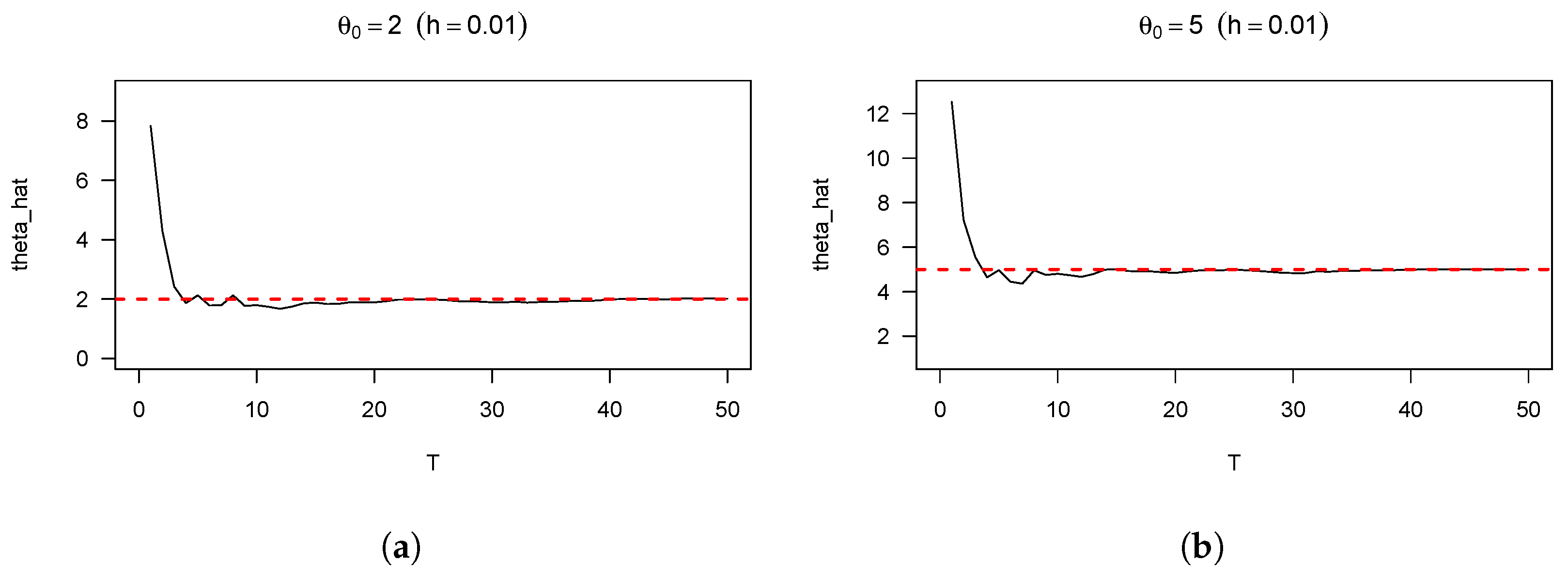
We simulate the trajectory of $\{X_t,t\ge 0\}$ using the Euler–Maruyama scheme over the interval $[0,T]$ with a total time of $T=50$ discretized into $N=5000$ steps. The estimator ${\widehat{\theta }}_N$ (where $T=Nh$) is then plotted against T for the true parameters ${\theta }_0=2$ and ${\theta }_0=5$.

For both subplots in Figure 1, the solid black line represents the estimated parameter $\widehat{\theta }$ computed from discrete observations, while the dashed red line indicates the true parameter value ${\theta }_0$. We can clearly observe that, regardless of whether the true parameter is set to ${\theta }_0=2$ or ${\theta }_0=5$, the estimator ${\widehat{\theta }}_N$ converges rapidly in the early iterations and quickly stabilizes at the level corresponding to the true parameter value (indicated by the red dashed line in the figures), demonstrating excellent rapid convergence and stability. This confirms the consistency of our proposed estimator.

For a comparison, the following table lists the values of $\widehat{\theta }\left(10\right),\widehat{\theta }\left(20\right),\dots ,\widehat{\theta }\left(50\right)$ for different choices of h. These results are based on 100 independent realizations of the process $\{X_t,t\ge 0\}$, each simulated via the Euler–Maruyama method, from which we obtain the average value of the estimator ${\widehat{\theta }}_N$ (see

Table 1. Average values of the estimator ${\widehat{\theta }}_N$ (${\theta }_0=2$).

h	T = 10	T = 20	T = 30	T = 40	T = 50
$2^{-6}$	2.0536 (0.2808)	2.0179 (0.1265)	2.0050 (0.0755)	2.0134 (0.0490)	1.9931 (0.0335)
$2^{-7}$	2.0767 (0.2403)	2.0015 (0.1131)	2.0119 (0.0736)	1.9886 (0.0577)	1.9974 (0.0497)
$2^{-8}$	2.0233 (0.2837)	1.9954 (0.1481)	2.0044 (0.0922)	2.0015 (0.0677)	1.9996 (0.0471)

Note. The non-parenthesized entries represent the mean values of the estimator, while the values in parentheses denote the standard deviations of the estimator.

).

It can be observed from the table that as the step size h decreases and the time horizon T increases, the average value of the estimator ${\widehat{\theta }}_N$ approaches the true parameter ${\theta }_0$. Furthermore, the standard deviation of ${\widehat{\theta }}_N$ decreases as T increases, which aligns with our theoretical consistency results.

7. Conclusions

In this paper, we have studied parameter estimation for a class of linear self-attracting diffusion processes with a drift coefficient of the form $-\theta \left({\int }_0^t(X_t-X_u)du\right)$. The estimation problem is investigated under both continuous and discrete observation schemes. Explicit formulas for the MLE and LSE are derived, and it is shown that the two estimators coincide in both continuous and discrete observations. The consistency and asymptotic distribution of the estimators ${\widehat{\theta }}_T$ and ${\widehat{\theta }}_N$ are established. Furthermore, the performance of ${\widehat{\theta }}_N$ is evaluated via Monte Carlo simulations using synthetic data generated from the model. A natural direction for future work is to investigate the properties of the estimators under generalized nonlinear settings. This would further extend our asymptotic results and address the challenges posed by nonlinear self-attracting diffusion processes, which we have identified as a promising research direction in the concluding discussion.

References

1. Cranston, M.; Le Jan, Y. Self attracting diffusions: Two case studies. Math. Ann. 1995, 303, 87–93. [Google Scholar] [CrossRef] [Scilit]
2. Durrett, R.T.; Rogers, L.C.G. Asymptotic behavior of Brownian polymers. Probab. Theory Relat. Fields 1992, 92, 337–349. [Google Scholar] [CrossRef] [Scilit]
3. Herrmann, S.; Scheutzow, M. Rate of convergence of some self-attracting diffusions. Stoch. Process. Their Appl. 2004, 111, 41–55. [Google Scholar] [CrossRef] [Scilit]
4. Yan, L.; Sun, Y.; Lu, Y. On the Linear Fractional Self-attracting Diffusion. J. Theor. Probab. 2008, 21, 502–516. [Google Scholar] [CrossRef] [Scilit]
5. He, J.; Guo, Q. An explicit method for the self-interacting diffusion driven by fractional Brownian motion under global Lipschitz conditions. Appl. Math. Lett. 2022, 134, 108379. [Google Scholar] [CrossRef] [Scilit]
6. Bishwal, J.P.N. Parameter Estimation in Stochastic Differential Equations; Lecture Notes in Mathematics; Springer: Berlin/Heidelberg, Germany, 2008; Volume 1923. [Google Scholar] [CrossRef] [Scilit]
7. Aït-Sahalia, Y. Maximum Likelihood Estimation of Discretely Sampled Diffusions: A Closed-form Approximation Approach. Econometrica 2002, 70, 223–262. [Google Scholar] [CrossRef] [Scilit]
8. Kasonga, R.A. The consistency of a non-linear least squares estimator from diffusion processes. Stoch. Process. Their Appl. 1988, 30, 263–275. [Google Scholar] [CrossRef] [Scilit]
9. Prakasa Rao, B.L.S. Asymptotic theory for non-linear least squares estimator for diffusion processes. Ser. Stat. 1983, 14, 195–209. [Google Scholar] [CrossRef] [Scilit]
10. Sun, X.; Yan, L.; Ge, Y. The Laws of Large Numbers Associated with the Linear Self-attracting Diffusion Driven by Fractional Brownian Motion and Applications. J. Theor. Probab. 2022, 35, 1423–1478. [Google Scholar] [CrossRef] [Scilit]
11. Jørgensen, E.S.; Sørensen, M. Prediction-based estimation for diffusion models with high-frequency data. Jpn. J. Stat. Data Sci. 2021, 4, 483–511. [Google Scholar] [CrossRef] [Scilit]
12. Mazzonetto, S.; Nieto, B. Parameters estimation of a threshold Chan–Karolyi–Longstaff–Sanders process from continuous and discrete observations. Scand. J. Stat. 2025, 52, 1670–1707. [Google Scholar] [CrossRef] [Scilit]
13. Han, J. Least Squares Estimation for Self-Attracting Diffusion with Discrete Observations. Adv. Appl. Math. 2019, 8, 1993–2001. [Google Scholar] [CrossRef]
14. Chen, X.; Lu, Y.; Yan, L. Least Squares Estimation for the Linear Self-Attracting Diffusion Driven by α-Stable Motions. Adv. Appl. Math. 2021, 10, 3969. [Google Scholar] [CrossRef]
15. Magnus, R. Essential Ordinary Differential Equations; Springer Undergraduate Mathematics Series; Springer International Publishing: Cham, Switzerland, 2023. [Google Scholar] [CrossRef] [Scilit]
16. Øksendal, B. Stochastic Differential Equations; Universitext; Springer: Berlin/Heidelberg, Germany, 2003. [Google Scholar] [CrossRef] [Scilit]
17. Kloeden, P.E.; Platen, E. Numerical Solution of Stochastic Differential Equations; Springer: Berlin/Heidelberg, Germany, 1992. [Google Scholar] [CrossRef] [Scilit]
18. Klebaner, F.C. Introduction to Stochastic Calculus with Applications, 3rd ed.; Imperial College Press: London, UK, 2012. [Google Scholar] [CrossRef] [Scilit]
19. Kutoyants, Y.; Pohlmann, H. Parameter estimation for Kalman-Bucy filter with small noise. Statistics 1994, 25, 307–323. [Google Scholar] [CrossRef] [Scilit]
20. Hu, Y.; Nualart, D. Parameter estimation for fractional Ornstein–Uhlenbeck processes. Stat. Probab. Lett. 2010, 80, 1030–1038. [Google Scholar] [CrossRef] [Scilit]
21. Yoshida, N. Estimation for diffusion processes from discrete observation. J. Multivar. Anal. 1992, 41, 220–242. [Google Scholar] [CrossRef] [Scilit]
22. Florens-zmirou, D. Approximate discrete-time schemes for statistics of diffusion processes. Statistics 1989, 20, 547–557. [Google Scholar] [CrossRef] [Scilit]
23. Casella, G.; Berger, R. Statistical Inference, 2nd ed.; Chapman and Hall/CRC: New York, NY, USA, 2024. [Google Scholar] [CrossRef] [Scilit]
24. Liptser, R.S.; Shiryaev, A.N. Statistics of Random Processes; Stochastic Modelling and Applied Probability; Springer: Berlin/Heidelberg, Germany, 2001; Volume 6. [Google Scholar] [CrossRef] [Scilit]
25. Rao, B.L.S.P. Semimartingales and Their Statistical Inference; CRC Press: Boca Raton, FL, USA, 2019. [Google Scholar] [CrossRef] [Scilit]
Figure 1. Estimated values of θ ^ against time horizon T for (a) θ 0 = 2 and (b) θ 0 = 5 (step size h = 0.01 ). The dashed red line denotes the true parameter value θ 0 .
Mathematics 14 01125 g001