Resource Allocation and Task Migration in DIMA-Oriented Mobile Edge Computing Systems

Abstract

Avionics systems are evolving from Integrated Modular Avionics (IMA) to Distributed Integrated Modular Avionics (DIMA), where distributed computing nodes are interconnected through real-time networks to support flexible resource sharing and latency-critical services. This architecture is highly consistent with the paradigm of Mobile Edge Computing (MEC), in which distributed edge resources collaboratively process computation workloads close to users to meet stringent real-time requirements. However, efficient task scheduling and migration remain key challenges in such distributed MEC platforms, since many existing approaches are designed for traditional centralized architectures and lack effective support for runtime workload dynamics and migration overheads. In this paper, we abstract the computing resource and task models for DIMA-oriented MEC systems and propose two algorithms: an Efficient Workload Scheduling Algorithm (EWSA) for workload placement and a Workload Migration Algorithm (WMA) for adaptive task relocation. CloudSim-based simulations show that the proposed methods significantly outperform the benchmark JIT-C approach in scheduling performance and migration efficiency, demonstrating their effectiveness for real-time distributed edge computing environments.

1. Introduction

With the rapid growth of computation-intensive and latency-sensitive services, distributed computing architectures are increasingly adopted to provide flexible resource sharing and real-time processing capabilities. In avionics systems, this evolution is reflected in the transition from Integrated Modular Avionics (IMA) to Distributed Integrated Modular Avionics (DIMA), where multiple distributed computing nodes are interconnected through real-time networks to support advanced onboard applications and system scalability [1]. Compared with traditional monolithic architectures, DIMA effectively reduces software–hardware coupling and improves deployment flexibility by enabling workloads to be scheduled and executed across distributed processing units [2,3].

From the perspective of system architecture, DIMA shares core characteristics with Mobile Edge Computing (MEC) [4]. MEC brings computation and storage resources closer to service requesters and allows distributed edge nodes to collaboratively process workloads, thereby meeting stringent latency requirements and improving service continuity [5,6]. In both DIMA and MEC-like distributed platforms, resource sharing among heterogeneous nodes and real-time networking capabilities enable flexible workload execution, while also introducing new challenges in workload orchestration and performance stability [2,5].

Despite the architectural advantages, efficient resource allocation and task management remain critical issues in distributed MEC platforms [7]. In particular, task scheduling and task migration are essential to ensure that workloads are executed within time constraints while maintaining high resource utilization [3]. However, existing scheduling approaches are often designed for centralized systems or assume relatively static execution environments. Such assumptions may limit their effectiveness when workload dynamics become significant or when migration overheads must be explicitly considered. In real-time distributed systems, inappropriate scheduling or migration decisions can lead to performance degradation, increased latency, and unnecessary resource consumption [8].

Therefore, the core problem addressed in this paper is how to jointly perform workflow scheduling and task migration in DIMA-oriented MEC platforms under dynamic workloads and potential resource failures, while explicitly accounting for migration overhead and real-time constraints. This problem is characterized by three coupled challenges: (i) distributed and heterogeneous resources that invalidate centralized scheduling assumptions; (ii) runtime workload variations and failures that undermine static execution models; and (iii) migration-induced overhead that must be carefully controlled to avoid deadline violations and performance degradation.

To address these challenges, this paper proposes a unified scheduling and migration framework for DIMA-oriented mobile edge computing systems. Specifically, we first abstract the computing resource and task workload models to characterize distributed nodes interconnected by real-time networks. Based on this modeling, two lightweight algorithms are developed: (i) an Efficient Workload Scheduling Algorithm (EWSA) for deadline-aware workload placement; and (ii) a Workload Migration Algorithm (WMA) for adaptive task relocation under runtime variations and resource failures. The proposed framework is evaluated using CloudSim-based simulations. Compared with the benchmark JIT-C approach, the results demonstrate significant improvements in scheduling performance and migration efficiency, validating the effectiveness of the proposed method for real-time distributed edge computing environments.

To bridge the gap between the limitations of existing scheduling approaches and the unique requirements of DIMA-oriented MEC systems, the main contributions of this paper are summarized as follows:

1.

DIMA-oriented MEC modeling: We abstract distributed computing resources and workload characteristics for DIMA-oriented mobile edge computing systems interconnected by real-time networks;

2.

Efficient scheduling algorithm: We propose EWSA to achieve efficient workload placement in distributed MEC platforms, improving scheduling effectiveness under resource constraints;

3.

Adaptive migration algorithm: We develop WMA to support adaptive task migration, explicitly addressing runtime workload dynamics and migration overheads;

4.

Simulation-based evaluation: CloudSim-based experiments are conducted to validate the proposed approach, showing consistent performance gains over the benchmark JIT-C method.

The remainder of this paper is structured as follows. Section 2 reviews related work, Section 3 describes the DIMA system model, Section 4 introduces the proposed scheduling algorithms, Section 5 presents simulation results, and Section 6 concludes the paper.

2. Related Works

With the rapid development of cloud, edge, and hybrid computing, efficient workflow scheduling has attracted extensive attention. Recent studies have combined Graph Neural Networks (GNNs) with Deep Reinforcement Learning (DRL) to enhance adaptability. For example, Gao et al. proposed a GNN-enhanced DRL framework for multi-task scheduling, improving resource utilization and completion controllability [9], while Yang et al. introduced GOODRL, integrating graph attention with offline–online DRL for dynamic workflows [10]. Cui et al. further developed a QoS-aware HEFT-LWOA hybrid method, achieving notable improvements under deadline constraints [11]. In parallel, traditional metaheuristics including GA, PSO, and ACO remain widely applied. Mikram et al. combined GA/PSO with HEFT to reduce makespan [12], Zhang et al. developed GMPSO to balance delay and energy [13], and Liu et al. proposed an ACO-based adaptive scheduler for heterogeneous environments [14]. In addition, distributed resource allocation has been extensively investigated in multi-agent systems, where decentralized optimization and consensus-based strategies have demonstrated superior scalability and robustness compared with centralized approaches [15]. However, most of these methods focus on generic agent coordination and do not explicitly consider workflow dependencies, migration overhead, or real-time constraints, which are critical in DIMA-oriented MEC avionics platforms. Although effective, these methods struggle with dynamic dependencies, parameter sensitivity, and verifiable timing guarantees. In avionics, model-driven optimizations under IMA/ARINC653 [16] and partition–communication co-scheduling for DIMA [3] have improved processor efficiency and latency control, yet they rely on static tables and lack runtime elasticity. Overall, existing methods are insufficient to meet the stringent real-time and fault-tolerance requirements of DIMA, motivating the need for efficient and adaptive scheduling strategies.

In distributed and edge computing environments, task migration has become a key mechanism for ensuring system robustness and service continuity. Recent research has also investigated deadline-aware task scheduling and offloading strategies in mobile edge computing, which consider both timing constraints and optimal resource allocation [17,18]. Additionally, safety-critical edge computing architectures have been proposed to ensure predictable latency and robust execution for real-time applications in distributed environments [19]. Recent surveys show that migration technologies are widely used in cloud–edge collaboration to address node failures, mobility, and dynamic resource variations, thereby improving system availability while maintaining QoS [20]. Tuli et al. proposed PreGAN, a preemptive migration prediction model based on generative adversarial networks to trigger migration proactively before faults occur [21]. Wang et al. further integrated migration cost into scheduling and optimized it using DRL to enhance reliability and resource utilization in cloud–edge environments [22]. Meanwhile, fault-tolerance studies have emphasized that mechanisms such as migration, replication, and retry exhibit diverse effectiveness across applications, requiring holistic design under system constraints [23]. In the avionics domain, research efforts have proposed standardized dynamic reconfiguration prototypes [8] and system-level fault propagation models [24], providing foundations for fault-tolerant DIMA architectures. However, these works mainly focus on communication and routing reconfiguration, lacking an integrated workflow-level scheduling–migration strategy. Moreover, existing solutions often rely on reactive migration without considering critical-path or priority-aware constraints, making them unsuitable for the stringent real-time requirements of avionics systems [23]. Hence, developing efficient, unified scheduling–migration mechanisms for DIMA remains an urgent need to ensure both real-time performance and fault tolerance.

In summary, existing studies have made progress in workflow scheduling and fault-tolerant migration but still lack an integrated framework suitable for DIMA avionics systems. To address these limitations, this paper proposes two complementary algorithms: the Efficient Workflow Scheduling Algorithm (EWSA), which introduces hierarchical task scheduling and balanced resource allocation to minimize workflow completion time under deadline constraints; and the Workflow Migration Strategy (WMS), which adopts a preemptive, critical-path-aware migration mechanism to ensure uninterrupted execution under resource failures. Together, these algorithms achieve a unified scheduling–migration framework compliant with ARINC 653 standards [16], enhancing the real-time performance, reliability, and robustness of DIMA-based avionics systems.

3. DIMA Avionics System Model

3.1. Computing Resource Model

In traditional avionics systems, each subsystem was designed with a single function, typically installed in separate cabinets with dedicated power supply, and developed using real-time embedded systems that were tightly coupled with hardware. In contrast, Integrated Modular Avionics (IMA) consolidates general-purpose software and hardware resources into a shared computing platform for multiple applications, while adopting partitioning mechanisms to ensure system safety and reliability. Building on this, the Distributed Integrated Modular Avionics (DIMA) architecture employs a distributed design in which computing resources are deployed across different locations of the aircraft and interconnected through a hard real-time communication network, thereby enabling hardware sharing at the system level.

In this study, we abstract the computing resources within DIMA systems. Each resource is characterized by parameters such as processor, memory, and bandwidth, where a processor may contain one or more cores, each with a fixed processing capability. A computing resource can host multiple subsystem tasks that share the underlying hardware. To prevent interference among tasks, the ARINC 653 standard introduces the concept of partitioning, as shown in Figure 1. By assigning different tasks to distinct partitions, both temporal and spatial isolation are achieved, which improves system fault tolerance and safety. Within each partition, multiple task processes share the allocated hardware resources, and their scheduling can be specified by system designers using policies such as First-Come-First-Served (FCFS) or Minimum Finish Time First (MFS). Accordingly, in our abstract modeling of DIMA resources, virtual partitions (VPs) are introduced to host task applications.

Furthermore, we assume that an aircraft contains multiple heterogeneous computing resources, each with different processor counts, processing speeds, and memory configurations. When exposed externally, these resources are virtualized into unified computing and storage services, interconnected by a real-time communication network and sharing sensor interfaces. As illustrated in Figure 2, computing services are provided in the form of diverse CS, featuring various CPU types and memory configurations. These virtual partitions (VPs) can be dynamically created or destroyed according to task requirements, while storage services are centrally allocated and managed by the local storage module. If two tasks $t_i$ and $t_j$ are assigned to different virtual partitions and require data transfer, the communication time is calculated as $TT\left(e_{ij}\right)=d_{ij}/\beta$, where $d_{ij}$ is the size of the data transferred from $t_i$ to $t_j$, and $\beta$ denotes the average bandwidth between partitions. If the two tasks are executed within the same partition, the transmission time is zero. In this work, scheduling among partitions on the same computing resource follows either a time-shared or space-shared strategy, while task processes within a partition are scheduled according to the FCFS policy.

3.2. Computing Platform Model

As shown in Figure 3, the computing platform model of the DIMA avionics system is designed to support workflow-oriented task scheduling, with the detailed task model described in the following subsection. The adopted platform model is similar to that presented in [25]. In this framework, aircraft resources are virtualized as service-oriented resources, and workflow execution planning proceeds through three stages. First, resource provisioning identifies and maps the required computing resources and configures the corresponding VmPartitions. Second, these partitions are dynamically instantiated on suitable physical computing resources, and task execution schedules are generated. Finally, during system operation, the physical resources are continuously monitored; in case of faults, the fault-handling module is invoked to ensure uninterrupted task execution.

Workflow tasks are typically associated with quality-of-service (QoS) requirements, such as deadline constraints and resource specifications. Deadline constraints define the latest completion time for a workflow, while resource specifications include requirements for memory, processing capacity, and I/O. Based on these inputs, the Workflow Management System (WMS) automatically identifies the necessary resources and maps the tasks to appropriate VmPartitions.

The WMS consists of three modules: the resource allocation and mapping manager, the workflow scheduler, and the execution manager. The resource allocation and mapping manager further includes two submodules: the resource capability estimator, which analyzes workflow structures to determine resource demands, and the mapping manager, which maps the identified demands to VmPartitions. The workflow scheduler assigns workflow nodes to execute within these partitions, while the execution manager tracks task execution, records the Real Start Time (RST) and Real Finish Time (RFT), and updates resource status information. This task-driven computing model supports dynamic adjustments of allocated resources during runtime.

In addition, the platform incorporates a resource scanning module, a fault-handling module, and a VmPartition management module. The scanning and fault-handling modules work together to detect resource failures and activate appropriate recovery strategies, whereas the VmPartition management module dynamically creates or destroys partitions on physical resources, thereby ensuring efficient utilization and reliable scheduling.

3.3. Task Model

In real-world aerial combat missions, the execution process of an aircraft is typically carried out in sequential steps. As shown in Figure 4, before striking a target, the aircraft must first complete a series of prerequisite tasks, including target detection, identification, and tracking, while also performing counter-reconnaissance during tracking to avoid exposure. Only after these preliminary tasks are completed can the strike mission be executed. During this process, tasks are often interdependent: successor tasks cannot start until all their predecessors are completed, whereas tasks that are ready can be executed concurrently.

Based on these characteristics, the mission is abstracted into a workflow model. As illustrated in Figure 5, a workflow application $W=(T,E)$ is represented as a directed acyclic graph (DAG), where $T=\{t_1,t_2,\dots ,t_n\}$ denotes the set of task nodes, and E represents the set of directed edges indicating data transfer or control dependencies. A dependency $e_{ij}$ specifies a precedence constraint such that if $(t_i,t_j)\in E$, task $t_j$ (the child task) cannot start until task $t_i$ (the parent task) is completed due to the required data transfer. A child task becomes executable only when all its parent tasks have finished and all dependency conditions are satisfied. The workflow deadline D defines the latest allowable completion time for the entire workflow. In this study, each task node is modeled as a computational unit with a fixed number of instructions and an associated output data size. As shown in Figure 5, each directed edge corresponds to the time required for data transmission between tasks.

3.4. Task Migration Model

In traditional avionics systems, subsystems are tightly coupled with specific hardware; once a computing resource fails, the associated functional modules become inoperative, which severely compromises system safety and reliability and may interrupt mission execution. In contrast, the DIMA architecture decouples applications from physical resources, allowing tasks to be flexibly scheduled on shared hardware.

As shown in Figure 6, when the resource scanning module detects a faulty computing resource (e.g., Resource 1), the VmPartition running on it also fails. The fault-handling module then migrates the affected partition to an available resource and restarts the corresponding tasks, thereby ensuring the continued execution of the workflow. During this process, the scanning and fault-handling modules operate cooperatively to maintain system functionality under failure conditions. The core of the task migration mechanism lies in selecting appropriate target resources and reinitializing tasks within the migrated partitions, thereby meeting real-time requirements and guaranteeing uninterrupted workflow execution.

4. Efficient Scheduling Algorithms for DIMA Avionics Systems

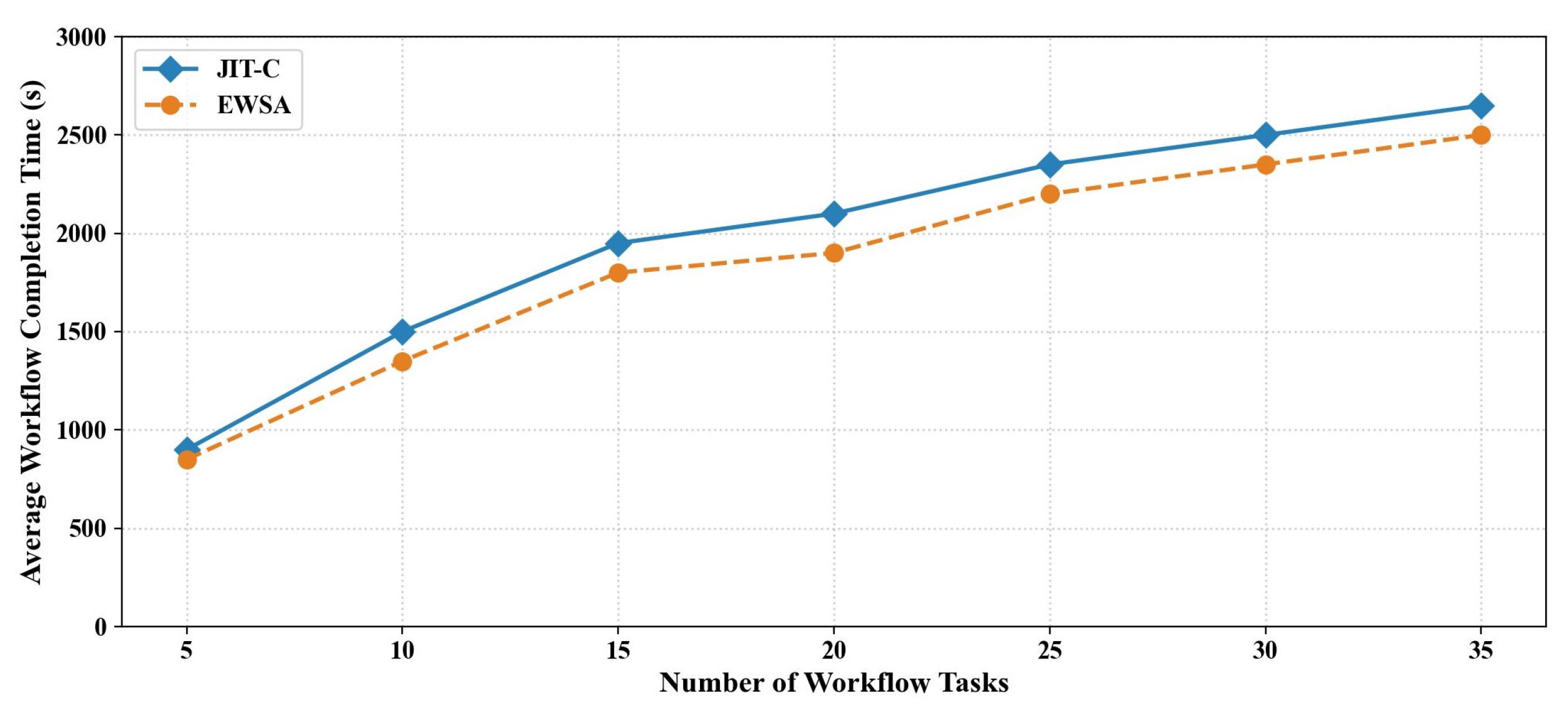
Jyoti Sahni and Deo Prakash Vidyarthi [26] proposed the Just-In-Time Cost (JIT-C) algorithm for workflow scheduling under deadline constraints. The key idea of JIT-C is to make effective scheduling decisions before tasks are ready for execution. To this end, the algorithm accounts for performance variations of virtual machines (VMs) in cloud platforms and employs a monitoring loop controller to track task progress, enabling dynamic adjustments of resource allocation and scheduling. While JIT-C demonstrates strong performance in real-time workflow scheduling within cloud environments, its applicability is limited by the centralized nature of cloud computing, making it unsuitable for parallel distributed systems. Motivated by this approach, we develop an efficient resource allocation and scheduling algorithm tailored to the DIMA architecture, which is designed for distributed computing environments.

4.1. Mathematical Preliminaries

In order to formally describe the scheduling and resource allocation problem in the DIMA architecture, it is necessary to define a set of mathematical notations and performance metrics. These notations capture task execution times, data transfer delays, scheduling constraints, and workflow deadlines, which together form the foundation for algorithm design and performance evaluation. By establishing these definitions, we ensure a precise and unified representation of the scheduling problem, thereby facilitating the development of efficient scheduling and migration strategies.

To model task execution in the DIMA architecture, we first define notations related to task execution time and communication delay. The execution time of a task $t_i$ on a virtual partition of type $vmpartitio{n}_v$ is expressed as $ET\left(t_i,v\right)$, and its minimum execution time $EMT\left(t_i\right)$ is determined by the fastest virtual partition type capable of executing it, as given in Equation (1). When tasks are mapped to different virtual partitions, communication delays arise from data dependencies, and the transfer time $TT\left(e_{ij}\right)$ is proportional to the data size $d_{t_i}$ and inversely proportional to the available bandwidth $\beta$ (Equation (2)). Based on these definitions, the earliest start time $EST\left(t_i\right)$ of a task depends on the completion of its parent tasks and associated data transfers (Equation (3)), while the earliest finish time $EFT\left(t_i\right)$ is obtained by summing its execution time and earliest start time (Equation (4)).

$$EMT\left(t_i\right)=\underset{v\in vmpartitio{n}_v}{min}\left\{ET\left(t_i,v\right)\right\}.$$

(1)

$$TT\left(e_{ij}\right)={\displaystyle \frac{d_{t_i}}{\beta }}.$$

(2)

$$EST\left(t_i\right)=\left\{\begin{array}{cc}0,\hfill & t_i=t_{entry},\hfill \\ \begin{array}{cc}\hfill & \underset{t_p\in t_i^{parent}}{max}\{EST\left(t_p\right)\hfill \\ \hfill & +MET\left(t_p\right)+TT\left(e_{p_i}\right)\},\hfill \end{array}\hfill & \mathrm{otherwise}.\hfill \end{array}\right.$$

(3)

$$EFT\left(t_i\right)=EST\left(t_i\right)+EMT\left(t_i\right).$$

(4)

At the workflow level, additional notations capture expected start and finish times, as well as deadline constraints. The expected finish time $EXFT\left(t_i\right)$ of tasks in the same layer can be estimated by averaging their execution times (Equation (5)), while the expected start time $EXST\left(t_i\right)$ is determined once all predecessor tasks are scheduled (Equation (6)). Under deadline constraints, the latest finish time $LFT\left(t_i\right)$ of a task is derived backward from the overall workflow deadline (Equation (7)), and the latest start time $LST\left(t_i\right)$ follows accordingly (Equation (8)). For the entire workflow, the minimum execution time $ME{T}_W$ corresponds to the critical path length (Equation (9)).

$$EXFT\left(t_i\right)=EXST\left(t_i\right)+{\displaystyle \frac{{\sum }_{j=1}^N\left(MET\left(t_j\right)\right)}{N}}.$$

(5)

$$EXST\left(t_i\right)=\left\{\begin{array}{cc}0,\hfill & t_i=t_{entry},\hfill \\ \begin{array}{cc}\hfill & \underset{t_p\in t_i^{parent}}{max}\hfill \\ \hfill & \{EXST\left(t_p\right)+TT\left(e_{pi}\right)\},\hfill \end{array}\hfill & \mathrm{otherwise}.\hfill \end{array}\right.$$

(6)

$$LFT\left(t_i\right)=\left\{\begin{array}{cc}D,\hfill & t_i=t_{exit},\hfill \\ \begin{array}{cc}\hfill & \underset{t_c\in t_i^{children}}{max}\{LFT\left(t_c\right)\hfill \\ \hfill & -MET\left(t_c\right)-TT\left(e_{ic}\right)\},\hfill \end{array}\hfill & \mathrm{otherwise}.\hfill \end{array}\right.$$

(7)

$$LST\left(t_i\right)=LFT\left(t_i\right)-EMT\left(t_i\right).$$

(8)

$$ME{T}_W=\underset{t_i\in W}{max}EFT\left(t_i\right).$$

(9)

In addition to the earliest time metrics, the actual execution times are defined to capture the real workflow completion process. The real start time $RST\left(t_i\right)$ of a task $t_i$ is determined by the latest completion time of its parent tasks plus the corresponding data transfer delay, as shown in Equation (10). The real finish time $RFT\left(t_i\right)$ of a task $t_i$ is then defined as the sum of its actual start time and the minimum execution time, as given in Equation (11). 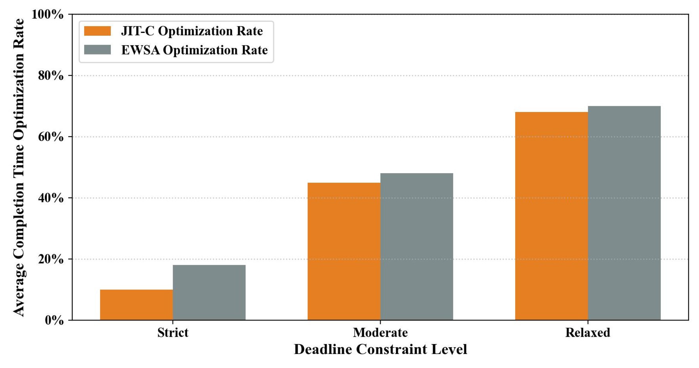Based on this, the total execution time $TE{T}_W$ of workflow W is defined as the maximum actual finish time among all tasks, as presented in Equation (12). Finally, the workflow completion time optimization rate $RATE$ is calculated as the relative improvement between the deadline D and the actual completion time, as expressed in Equation (13).

$$RST\left(t_i\right)=\underset{t_p\in t_i^{parent}}{max}RFT\left(t_p\right)+TT\left(e_{pi}\right).$$

(10)

$$RFT\left(t_i\right)=RST\left(t_i\right)+MET\left(t_i\right),$$

(11)

$$TE{T}_W=\underset{t_i\in W}{max}RFT\left(t_i\right),$$

(12)

$$RATE={\displaystyle \frac{TE{T}_W-D}{D}}.$$

(13)

4.2. Efficient Workflow Schedule Algorithm (EWSA)

When scheduling a workflow W, the first step is to verify whether the specified deadline D is feasible. If the deadline is infeasible, the scheduling problem has no valid solution and D must be reassigned. Once feasibility is confirmed, the objective becomes minimizing the total execution time $TE{T}_W$ of workflow W while satisfying real-time constraints.

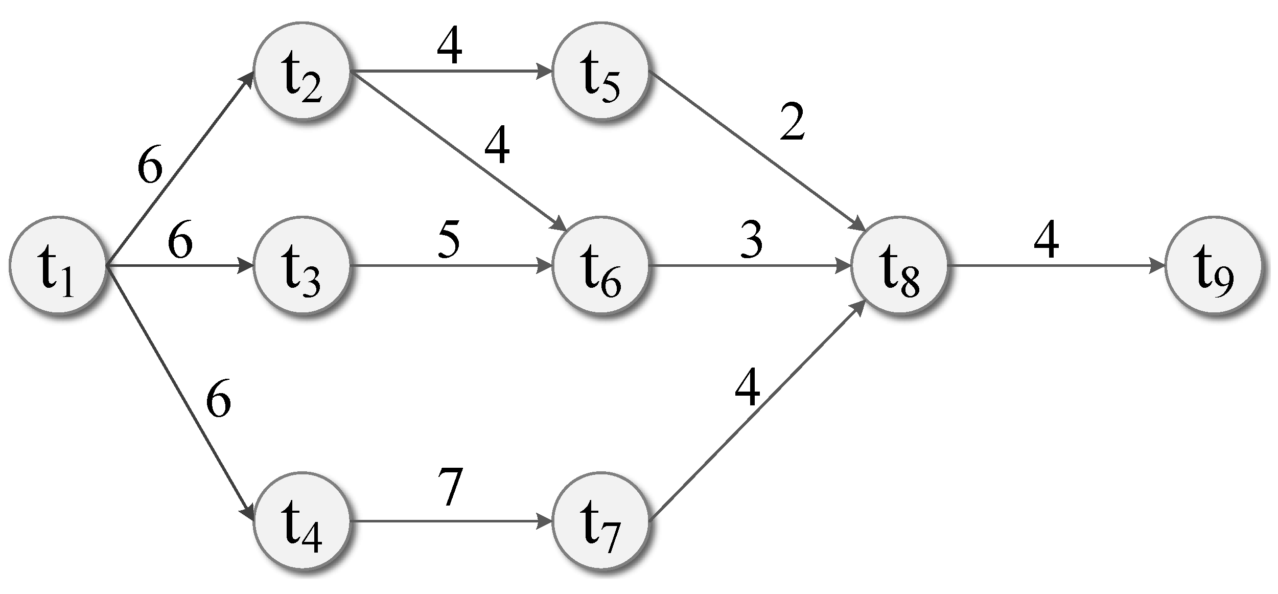
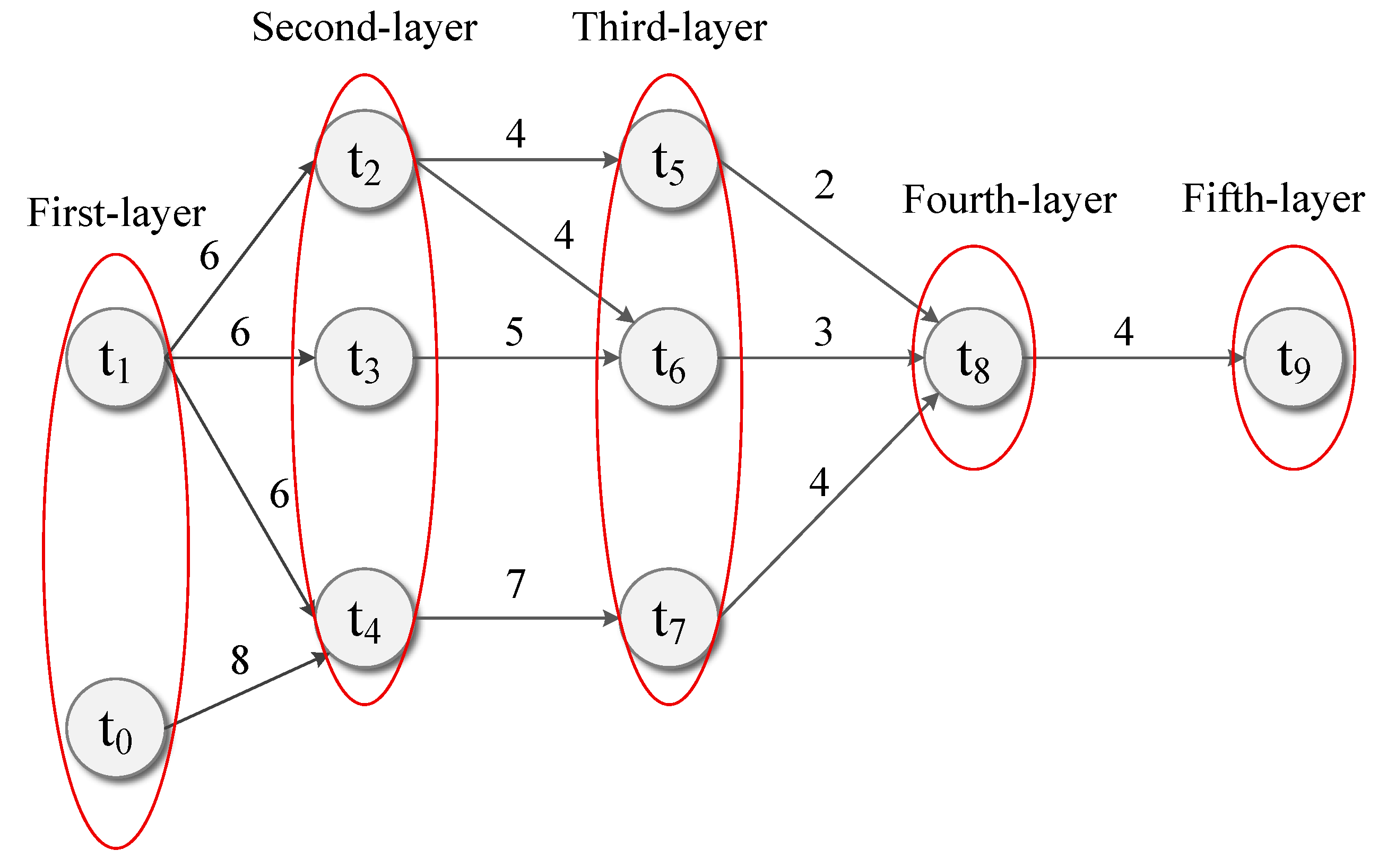
As illustrated in Figure 7, workflow tasks are executed in a hierarchical order, where a task $t_i$ cannot start until all its parent tasks are completed and the required data have been transferred. For example, task $t_4$ must wait for tasks $t_0$ and $t_1$ to finish and deliver their results before execution. Similarly, the execution and transmission times of tasks in one layer directly affect the scheduling of tasks in the subsequent layer. For instance, the completion of first-layer tasks $t_0$ and $t_1$ determines the execution readiness of second-layer tasks $t_2$, $t_3$, and $t_4$.

To reduce waiting time for successor tasks, we adopt a resource-balancing strategy such that the sum of execution and transmission times among tasks in the same layer remains approximately aligned. For example, the execution of task $t_6$ depends on the completion of parent tasks $t_2$ and $t_3$. To avoid long idle periods, their completion times are balanced to satisfy $ET\left(t_2\right)+TT\left(t_2\right)$$\approx ET\left(t_3\right)+TT\left(t_3\right)$. This is achieved by allocating more computing resources to tasks with larger workloads so they finish earlier, while assigning fewer resources to smaller tasks to prevent premature completion and reduce unnecessary system occupancy.

Building on this principle, we propose the Efficient Workflow Scheduling Algorithm (EWSA). As outlined in Algorithm 1, the workflow W is scheduled over the available computing resources of the aircraft platform. The process begins with initialization through the $Initialize\left(\right)$ function (line 2), followed by the computation of the minimum execution time $MET$, data transfer time $TT$, and earliest start time $EST$ for each task using Equations (1)–(3). Tasks on the critical path are then identified, and the overall minimum execution time of workflow W is computed using Equation (9) to determine its schedulability.

Algorithm 1: Efficient Workflow Schedule Algorithm (EWSA)

When the workflow W is deemed schedulable within its deadline D, the Pre-processing() algorithm (as shown in Algorithm 2) is first applied to optimize the workflow. This procedure updates the minimum execution time $MET$, latest finish time $LFT$, and latest start time $LST$ of each task node using Equations (1), (7) and (8), and employs the $\mathit{analysisLevel}\left(\right)$ function (line 7) to determine task levels. For tasks at the same level, the $\mathit{OptimalVmPartitionMapping}\left(\right)$ algorithm (as shown in Algorithm 3) assigns them to appropriate virtual partitions (VmPartition), thereby generating an initial scheduling plan. Subsequently, the $\mathit{SheduleAviationCloudlet}\left(\right)$ function (lines 13–17) within the scheduling management module executes the actual scheduling, dynamically instantiating the corresponding VmPartition on the aircraft’s computing resources. The execution manager then monitors the task execution, recording the real start time $RST$ and real finish time $RFT$. Once a task is completed, the execution manager cooperates with the scheduler to release the allocated resources by destroying the corresponding VmPartition.

During the dynamic creation of VmPartition, resource shortages may occur. In such cases, the configuration of VmPartition must be adapted under the following constraints:

1.

The expected finish time of task $t_i$ must not exceed its latest finish time, i.e., $EXFT\left(t_i\right)\le LFT\left(t_i\right)$;

2.

For all child tasks $t_c\in t_i^{children}$, it must satisfy that $EXFT\left(t_c\right)\le LST\left(t_c\right)$.

The Pre-processing() algorithm reduces inter-task communication overhead by merging serial task nodes via a queue-based mechanism and updating their dependencies. The $\mathit{OptimalVmPartitionMapping}\left(\right)$ algorithm (as shown in Algorithm 3), on the other hand, maps tasks at the same level to virtual partitions and binds them with task identifiers. It first employs the $\mathit{caculateAverageExecutionTime}\left(\right)$ function (line 2) to compute the average expected execution time based on Equations (4) and (5), and then uses the $\mathit{allocateResourceType}\left(\right)$ function (line 8) to assign computing resources according to the difference between the expected finish time and expected start time. In cases where $EXFT\left(t_i\right)\ge EXSF\left(t_i\right)$, the expected finish time is appropriately extended, effectively shrinking the allocated resources of the corresponding VmPartition, thereby ensuring the feasibility and efficiency of the scheduling plan.

Algorithm 2: Pre-processing(W)

Algorithm 3: $\mathit{OptimalVmPartitionMapping}\left(taskList\right)$

4.3. Workflow Migration Algorithm (WMA)

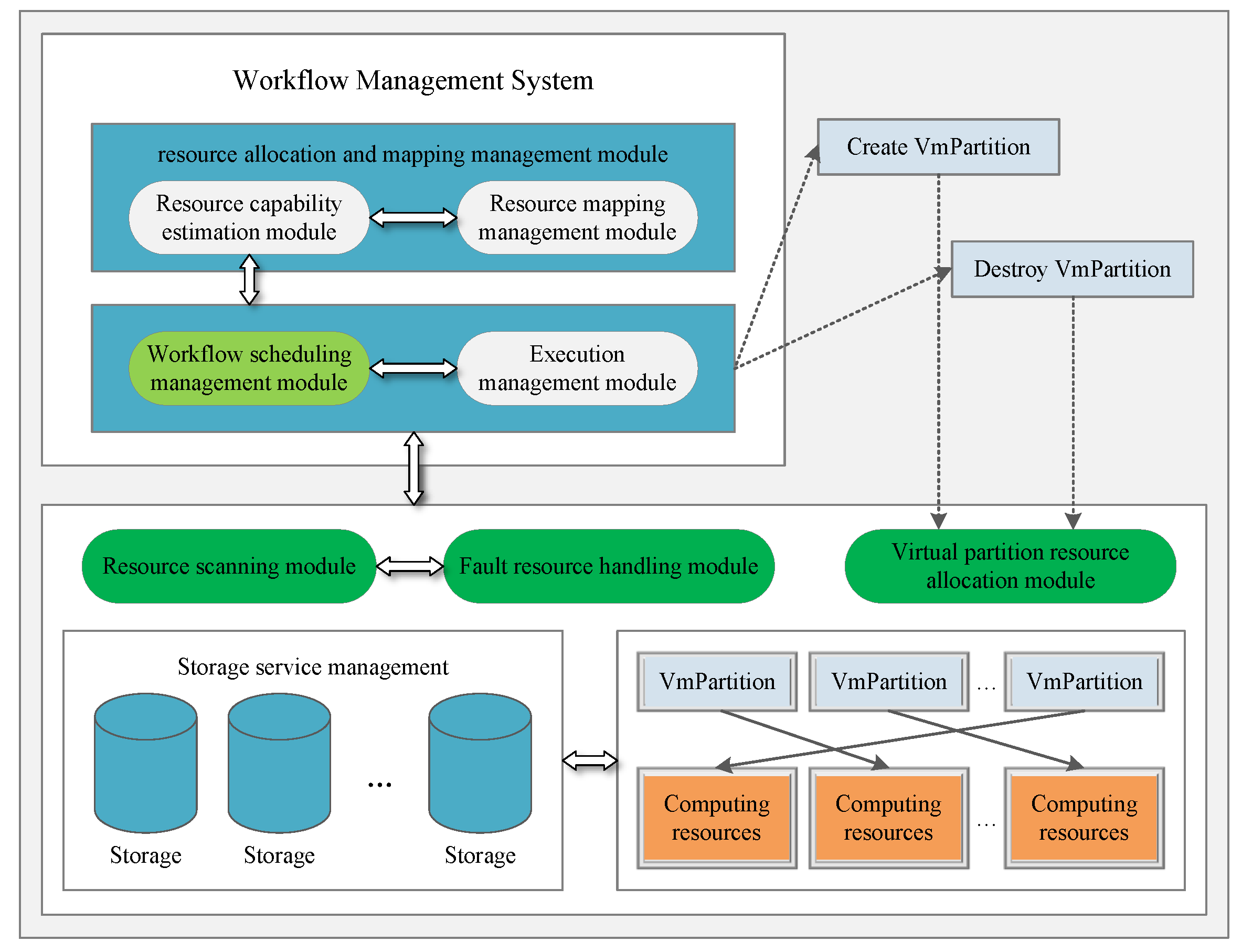
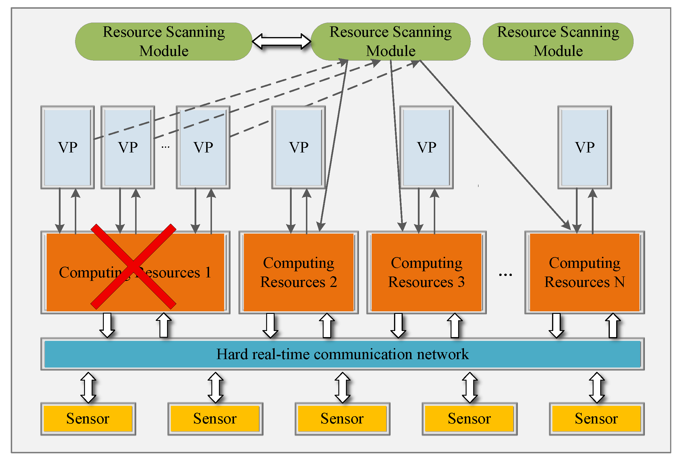
The workflow migration algorithm consists of two main components: the resource scanning module and the fault resource handling module. The resource scanning module periodically monitors the status of computing resources through a fixed triggering function. Once a faulty resource is detected, it invokes the fault resource handling module, which executes the migration process to ensure the continuous execution of workflow tasks.

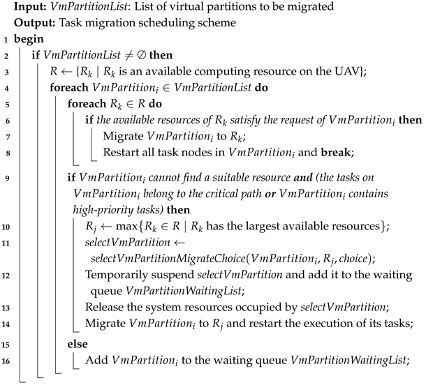
During the migration of a virtual partition (VmPartition) to an alternative computing resource, the system may encounter situations where the available capacity of the target resource is insufficient. To address this issue, the proposed approach adopts a preemptive mechanism when the tasks running on VmPartition belong to the critical path (i.e., the longest execution path) or are assigned special priority. In such cases, some of the tasks occupying the target resource are preempted and suspended, thereby ensuring the successful migration and execution of the current critical task.

The proposed Workflow Migration Algorithm (WMS) serves as the core of the fault resource handling module. It is specifically designed to cope with resource failures during mission execution by migrating tasks from faulty resources to alternative ones, thereby guaranteeing the reliable execution of workflow W. This algorithm operates in coordination with the resource scanning module: once a failure is detected, the VmPartition on the faulty resource is passed to the handling module, which executes the migration and reconfiguration process as illustrated in Algorithm 4. In practice, the algorithm traverses all available computing resources (lines 5–8); if a suitable resource $R_i$ is found, the VmPartition is directly migrated to $R_i$, and its tasks are restarted. If no suitable resource is available, the algorithm applies $\mathit{selectVmPartitionMigrateChoice}\left(\right)$ (lines 10–14) to select partitions for suspension and add them to a waiting queue. In this study, the function implements two strategies: (i) selecting the partition with the minimum resource usage, or (ii) selecting the partition with the longest task execution time.

Algorithm 4: $\mathit{WorkflowMigrationAlgorithm}\left(VmPartitionList\right)$

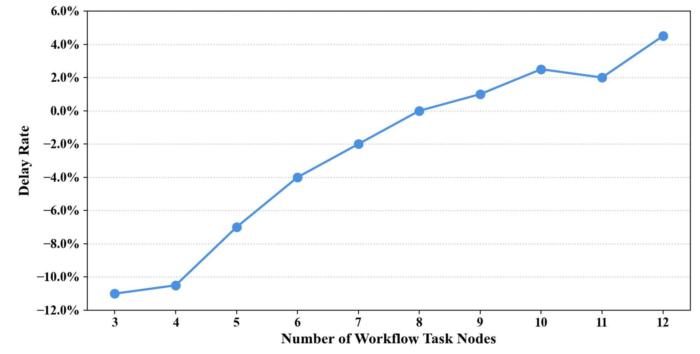
Once tasks release resources upon completion, the fault resource handling module gives priority to scheduling tasks in the waiting queue, thereby reducing delays and maintaining system continuity. Although preemptive migration may result in a longer overall workflow completion time, it ensures reliable task execution under resource failure conditions. Simulation results further demonstrate that in workflows with relatively simple dependency structures, the delay caused by migration is more significant, whereas in more complex workflows, the delay is reduced and may even lead to improved performance in certain cases.

4.4. Computational Complexity Analysis

Let N denote the number of workflow tasks, E the number of dependency edges in the DAG, and R the number of available computing resources. For Algorithm 1 (EWSA), the preprocessing stage traverses each task and dependency once, resulting in a complexity of $O(N+E)$. The subsequent level-based scheduling performs resource mapping for tasks at each level. In the worst case, all tasks belong to a single level, and the mapping procedure scans all tasks, leading to $O\left(N\right)$ per level. Since the number of levels is bounded by N, the overall complexity of EWSA is $O(N^2+E)$, which can be simplified to $O\left(N^2\right)$ for dense workflows. For Algorithm 4 (WMA), each virtual partition is checked against all available computing resources to identify feasible migration targets. Therefore, the migration procedure has a worst-case complexity of $O(P\times R)$, where P is the number of virtual partitions (with $P\le N$). This yields an upper bound of $O\left(NR\right)$. Both algorithms operate in polynomial time and are suitable for large-scale task scheduling and resource management scenarios. Moreover, EWSA is designed as a lightweight heuristic without iterative optimization loops, while WMA is triggered only upon resource failures, which further limits its runtime overhead in practical deployments.

To further assess the practicality of the proposed algorithms, we compare their computational complexity with representative categories of existing methods discussed in Section 2, as shown in

Table 1. Computational Complexity Comparison.

Methods	References	Technique	Complexity
Learning-based	[9,10]	DRL	Iterative training and inference
Metaheuristic	[12,13,14]	GA/PSO	$O\left(G{N}^2\right)$
Static avionics	[3,16]	Offline Table	Offline/static
EWSA & WMA	–	Heuristic	$O\left(N^2\right)$, $O\left(NR\right)$

. Learning-based scheduling approaches, such as DRL- or GNN-assisted methods, rely on iterative training and online inference of deep neural networks, which introduce non-negligible computational overhead and may limit real-time applicability [9,10]. Metaheuristic-based schedulers, including GA-, PSO-, and ACO-based methods, typically perform population-based iterative searches, resulting in computational complexity on the order of $O\left(G{N}^2\right)$ or higher, where G denotes the number of iterations [12,13,14]. In contrast, the proposed EWSA and WMA operate in polynomial time with worst-case complexities of $O\left(N^2\right)$, respectively, where N is the number of tasks and R is the number of computing resources. Moreover, unlike static avionics scheduling methods that rely on offline configuration and lack runtime adaptability [3,16], the proposed framework supports efficient online scheduling and migration, making it suitable for large-scale, real-time DIMA-oriented MEC systems.

5. Simulation and Results Analysis

5.1. Simulation Configuration

The proposed DIMA resource model, task model, computing platform model, and scheduling algorithms were implemented in the CloudSim simulation toolkit. To accommodate the characteristics of DIMA architectures, CloudSim was extended and customized within the Eclipse development environment. On this modified platform, the proposed models and algorithms were integrated and evaluated. The hardware configuration of the physical host is listed in

Table 2. Simulation Hardware Environment.

Name	Configuration
Processor	Intel(R) Core(TM) i7-4510U CPU @ 2.00 GHz 2.60 GHz
RAM	8.00 GB
Hard Disk	1 TB
Operating System	Windows 10 (64-bit)
Display	Lenovo Laptop Display (15.6 inch)

.

In the simulation setup, the aircraft is assumed to contain ten physical computing resources, classified into homogeneous and heterogeneous types. Homogeneous resources have identical processing and memory configurations (

Table 3. Homogeneous Computing Resource Information.

Quantity	Cores	Processing Power (GHz)	RAM (GB)
10	2	4	8

), while heterogeneous resources differ in their computational capacities (

Table 4. Heterogeneous Computing Resource Information.

Resource ID	Cores	Processing Power (GHz)	RAM (GB)
#1	1	2	4
#2	1	4	8
#3	1	6	16
#4	2	4	8
#5	2	8	16
#6	2	12	32
#7	4	8	16
#8	4	16	32
#9	8	16	32
#10	8	32	64

). The average bandwidth between virtual partitions (VmPartitions) is set to 200 MBps. Additionally, three baseline configurations of VmPartitions are defined (

Table 5. Baseline Configuration Types of VmPartitions.

VmPartition Type	Cores	Processing Power (GHz)	RAM (GB)	Storage (GB)
Small	1	1	1.7	160
Medium	1	2	3.75	410
Large	2	4	7.5	840

), and the resource scanning interval of physical resources is fixed at 200 s.

For performance evaluation, each workflow W is assigned a deadline. To analyze scheduling performance under different real-time constraints, deadlines are defined using Equation (14), where $ME{T}_W$ denotes the minimum execution time of workflow W, and $\mu$ is the deadline factor [26]. Based on the value of $\mu$, deadlines are categorized as strict ($0\le \mu <1.5$), moderate ($1.5\le \mu <3$), and relaxed ($3\le \mu <4.5$). Workflows are randomly generated, with task sizes ranging from 5 to 35 nodes $\{5,10,15,20,15,30,35\}$. The instruction count of each task node is uniformly distributed in the range $[2.5\times {10}^5,5\times {10}^5]$, while the data volume transferred between tasks lies within $[2\times {10}^2,5\times {10}^2]$ MB. Each workflow configuration is executed 100 times, and the average results are reported to evaluate algorithm performance.

$$DeadlineD=(1+\mu )\times ME{T}_W.$$

(14)

5.2. Experimental Results and Analysis

Based on the experimental configuration described in Section 5.1, simulations were conducted on the modified CloudSim platform to evaluate the proposed algorithms in terms of average completion time, optimization rate, and migration delay rate. The proposed ESWA algorithm is developed as an extension of the JIT-C algorithm to accommodate the characteristics of the DIMA architecture, while the original JIT-C serves as the benchmark for comparative analysis.

5.2.1. Average Completion Time

As shown in Figure 8, the proposed EWSA algorithm consistently outperforms the JIT-C algorithm in terms of average completion time. With the increase in the number of workflow tasks, the completion time of both algorithms grows, yet EWSA maintains a clear advantage. This improvement stems from EWSA’s ability to evaluate resource demands at each task level, thereby allocating more computing resources to tasks on the critical path, while allowing non-critical tasks more flexible execution time without delaying subsequent tasks. Consequently, resource allocation under the DIMA architecture becomes more balanced, leading to a reduction in critical path execution time.

5.2.2. Optimization Rate

The experiments evaluate algorithm performance under different deadline constraints, namely STRICT, MODERATE, and RELAXED. As shown in

Table 6. Workflow Scheduling Performance: Success and Optimization Rates.

Deadline	Algorithm	Metric	5	10	15	20	25	30
STRICT	JIT-C	Success Rate (%)	78	76	74	73	74	75
		Optimization Rate (%)	5	5	5	5	4	5
	EWSA	Success Rate (%)	90	89	91	86	88	87
		Optimization Rate (%)	17	14	15	15	12	12
MODERATE	JIT-C	Success Rate (%)	100	100	100	100	100	100
		Optimization Rate (%)	41	42	42	42	41	42
	EWSA	Success Rate (%)	100	100	100	100	100	100
		Optimization Rate (%)	44	45	44	45	46	44
RELAXED	JIT-C	Success Rate (%)	100	100	100	100	100	100
		Optimization Rate (%)	70	70	70	69	67	68
	EWSA	Success Rate (%)	100	100	100	100	100	100
		Optimization Rate (%)	70	72	70	70	70	70

, under STRICT deadlines, the scheduling success rate of JIT-C is approximately 75%, whereas EWSA achieves 90%. This improvement arises from EWSA’s ability to dynamically adjust task resource requests according to the availability of platform resources, ensuring that most requests are satisfied. Under MODERATE and RELAXED deadlines, both algorithms achieve a 100% success rate, as the extended deadlines provide sufficient flexibility for task scheduling.

The optimization rate is calculated relative to workflow deadlines, as defined in Equation (13). To visualize the results, optimization performance is presented in bar charts (Figure 9). Under STRICT deadlines, EWSA improves the optimization rate by about 10% compared to JIT-C, while under MODERATE and RELAXED deadlines, the improvement is around 3%. As the deadline constraints are relaxed, JIT-C is able to identify suitable resource allocations, leading to diminishing differences, while EWSA’s optimization advantage gradually approaches saturation. Moreover, with the increase in task nodes, workflow dependencies become more complex, reducing concurrency and making scheduling closer to sequential execution, which in turn decreases the overall optimization potential.

5.2.3. Migration Delay Rate

To address potential computing resource failures during aircraft mission execution, we introduce the WMA task migration algorithm to ensure workflow continuity and enhance the robustness of DIMA avionics systems. In the simulations, we evaluated the efficiency of task migration and reorganization by configuring both the fault occurrence time and the number of failed resources. Specifically, failures were triggered 400 s after simulation start, with the number of faulty resources randomly selected between [1, 8]. As illustrated in Figure 10, the figure visualizes the impact of migration on workflow execution under different task scales. When the number of workflow tasks is small and dependency relations are simple, task migration and reorganization lead to a relatively high delay rate, approximately –11%. However, as the number of tasks increases and dependency structures become more complex, the delay rate gradually decreases, and in some cases, the completion time is slightly improved (around 2%). This occurs because higher dependency complexity reduces the degree of parallelism among tasks at the same level, making the overall workflow execution closer to a serial process, thereby mitigating the relative overhead introduced by migration.

In summary, although task migration and reorganization in the DIMA architecture may slightly compromise strict real-time constraints, they provide significant advantages over traditional avionics systems by ensuring workflow completion under resource failures. The proposed EWSA scheduling algorithm and WMA migration algorithm consistently outperform the JIT-C baseline in terms of efficiency, robustness, and adaptability. These results highlight that our approach not only enhances resource utilization and fault tolerance in distributed avionics systems but also aligns with the architectural principles of DIMA and conforms to the ARINC653 avionics standard.

6. Conclusions

This paper addressed workflow scheduling and migration in DIMA-oriented mobile edge computing systems. We developed an efficient workflow scheduling algorithm (EWSA) to optimize task execution under deadline constraints and a workflow migration strategy (WMA) to ensure task continuity under resource failures. Experimental results on an extended CloudSim platform demonstrated that the proposed methods outperform the baseline JIT-C algorithm in terms of completion time, optimization rate, and system reliability, highlighting their effectiveness in improving both efficiency and resilience of next-generation avionics platforms. Although motivated by DIMA avionics systems, the proposed framework is based on generic distributed resource and workflow models and can be extended to other real-time MEC scenarios with similar latency and reliability requirements.