The Robust LM Test for Spatial Effects in a Common-Factor Scenario: A Review and Monte Carlo Results

Abstract

I address the empirical properties of the popular robust LM tests of Anselin et al. (1996) for the specification of spatial models when employed in a scenario characterized by unobserved common factors with idiosyncratic loadings. I describe the small-sample behavior by way of simulation, without deriving any analytical results. I build upon the analysis in Millo (2025), extending it from homogeneous time effects to common factors with heterogeneous loadings, a very common setting, e.g., in empirical macroeconometrics. As in the former paper, I document severe distortions in the empirical size and power of the spatial tests when omitting the common factors. Then, I evaluate the strategy of controlling for the heterogeneity by augmentation, including simple (TFE) or interactive fixed effects (IFE) in the test specification. Unlike the homogeneous cases, I find that the correction to the test power may come at a non-negligible cost in terms of size distortion: for some combinations of sample sizes, in particular for short panels, IFE-corrected tests can be severely over-rejecting. This is traced back to a well-known incidental parameter problem. TFE-corrected tests can instead suffer from low power. Nevertheless, either form of augmentation is preferable to ignoring time effects when potentially present.

1. Introduction

The literature on panels with unobserved common factors and idiosyncratic loadings (also “interactive fixed effects” because they can be represented through the interaction of time dummies with individual fixed effects) has mainly concentrated on consistent estimation of the impacts of regressors rather than on spatial patterns, ever since the seminal contributions of Pesaran [1] and Bai [2]. Although in a later paper Pesaran and Tosetti [3] considers the coexistence of common factors with spatial error correlation, the CCE estimator of Pesaran [1] is established as being consistent even in the presence of spatial correlation.

Holly et al. [4] is among the first papers in the common-factor literature to address the spatial process as a phenomenon of interest rather than just a nuisance in estimation. Standard spatial estimators will generally be inconsistent when a (potentially endogenous) common-factor structure is neglected. Given their consistency under common factors, CCE estimators do instead yield residuals that can be used for estimating the spatial diffusion pattern in the remainder errors, which can be of interest in its own right; on this basis, the authors estimate a spatial autoregressive model for the local diffusion of house prices after controlling for common, nationwide factors. This two-step process has been formalized in Bailey et al. [5] (see also [6], for a different approach in the same spirit).

The subsequent literature has developed the joint estimation of spatial models with common factors, most notably in Shi and Lee [7], who derived quasi-maximum likelihood estimators, and Yang [8], who proposed several IV/GMM methods, applying them, again, to US house prices. On the whole subject, see also the survey in Elhorst [9].

More modestly, this note addresses the issue of specifying the spatial process through the popular robust Lagrange multiplier (RLM) tests of Anselin et al. [10], when the data-generating process may contain an unobserved common-factor component. In particular, I consider the choice between a spatial lag (SAR) process (the outcome in one location depends on the outcome in neighboring ones) and a spatial error (SEM) process (the innovations in one location depend on those of the neighbors, so that shocks spread in space). I assess the viability of a specification strategy based on the RLM tests for the spatial process in the defactored data by augmenting the test model with interactive fixed effects, analogous to the fixed effects augmentation strategy proposed in Millo [11].

Spatial panels commonly present a number of features in addition to the spatial effects proper: most prominently, individual and/or time effects, of either “fixed” type (i.e., potentially correlated with the regressors) or “random” (i.e., uncorrelated). Each one of these features, if not properly taken into account, can invalidate the RLM, which (a) is based on some maintained specification hypotheses (on the form of the data-generating process); (b) relies on the byproducts—the residuals—of an estimation procedure based on assumptions on the error terms. In principle, under omitted and correlated individual heterogeneity (fixed effects), the OLS residuals on which the test is based are inconsistently estimated, and the whole procedure is inappropriate tout court; nevertheless, the bias from uncorrelated individual heterogeneity has been shown to potentially invalidate the RLM as well, by breaking the hypothesis of i.i.d. errors on which the tests are based. The bias from omitted time effects is even more serious, because the cross-sectional correlation they introduce is easily mistaken for spatial correlation.

Millo [11] documented both the above biases and showed how performing the tests on the residuals of a model in which individual and/or time effects have been controlled for through individual and/or time dummies (or, equivalently, “within” transformations of the data) does recenter the test statistics, restoring test size (the frequency of false rejections) to the designed level, so that the RLM, despite having been designed for cross-sections, can be safely employed in homogeneous panel data settings.

In the case of unobserved common factors with heterogeneous loadings, this suggests the analogous strategy of augmenting the test equation with the interaction of individual and time dummies (interactive fixed effects). The above paper mentions some encouraging preliminary results from simulations, leaving a thorough assessment of such a strategy for future work, which I take up here.

Unfortunately, upon closer inspection, I find only partially satisfactory results, so that the present paper works as a word of caution and as a partial correction to the optimistic view of Millo [11] (Experiment 4c, p.13): unlike the homogeneous time fixed effects case, where an augmentation strategy does, in general, work well, preserving the good properties of the RLM tests, in the case of common factors with heterogeneous loadings the same finds a natural limit in the large number of incidental parameters it would introduce. Test statistics are indeed recentered, but the test size turns out to be severely, albeit uniformly and predictably, distorted for panels with a very small time dimension (“short panels”). A tradeoff between simplicity and effective control emerges, whereby—in the particular case of short panels—the simple time dummies augmentation fares relatively well in comparison, so that a researcher may therefore be better off controlling for unobserved time heterogeneity in test equations by simple time dummies rather than by adding interactive fixed effects. For larger, although still modest, time dimensions, the interactive fixed effects augmentation does work much better, becoming an entirely viable strategy; the range of the latter includes the majority of empirical works considered in recent surveys of the empirical spatial panel literature (see Footnote 14 in [11]).

In the following sections, I first present the general, encompassing setting for a panel model with spatial dependence of both the lag and error type, individual heterogeneity, and common time effects with idiosyncratic loadings; then the RLM test statistics, discussing how they were derived in a much simpler framework, and the various augmentation strategies proposed to adapt them to this more general framework. Next, I present the simulation strategy I employ for assessing the empirical behavior—in terms of test size and power—of the RLM, both “plain vanilla” and augmented, under the common-factor scenario. Then I present, graphically, the results from two Monte Carlo experiments: the first, based on two real-world geographies, motivates the paper by comparing three strategies—no correction, time fixed effects augmentation, and interactive fixed effects augmentation—in the test equation; the second, based on two synthetic, regular geographies (which, as such, can be extended and adapted at will), systematizes the investigation across different sample sizes in space (increasing-domain) and time, with the aim of inferring regularities in test behavior. Next, I briefly discuss the limitations of the present study and sketch potential directions for future work. I conclude by summarizing the results and presenting takeaways for empirical spatial panel work.

2. The Model and Tests

In the context of a spatial panel with both lag and error-type dependence, I follow the mainstream cross-sectional dependence literature (see, e.g., [3]) in modeling the influence of unobserved time heterogeneity common to all units through a structure of unit-specific, time-invariant factor loadings, so that time fixed effects can be seen as a special case of common factors where all loadings are constrained to 1.

Elaborating on Millo [11] (the simulation scenario has two main differences from that of Millo [11]: the addition of heterogeneous factor loadings and the omission of serial error correlation), I consider a panel of N individual units over T periods, introducing individual heterogeneity through a vector $\mu$ of individual-specific, time-invariant effects and time heterogeneity through another vector $\eta$ of effects that are time-specific and invariant over individuals. The idiosyncratic common-factor structure is represented by the interaction of the vector of N individual factor loadings $\gamma$ with that of T time effects $\eta$ (the common-factor structure simplifies to homogeneous time effects if $\gamma ={ı}_N$). Spatially autoregressive processes are present in both the dependent variable $\mathbf{y}$ and the error $\mathbf{e}$. This setting allows for cross-sectional dependence (XD) of two different kinds: weak cross-sectional dependence (XWD), which disappears asymptotically as the cross-sectional sample size grows in an “increasing domain” fashion, i.e., as the boundaries expand to include new regions (as opposed to “fill in” asymptotics, where the number of cross-sectional units grows because of a finer subdivision within the same geography); and also for strong (XSD), or “factor-type dependence”, which persists irrespective of the distance between units.

In vector form, with cross sections stacked—as is standard in the spatial panel literature—we have the following:

$$\begin{array}{c}\mathbf{y}=\rho (I_T\otimes W)\mathbf{y}+\beta \mathbf{X}+\mathbf{u}\hfill \\ \mathbf{u}=({\mathit{𝚤}}_T\otimes \mu )+(\eta \otimes \gamma )+\mathbf{e}\hfill \\ \mathbf{e}=\lambda (I_T\otimes W)\mathbf{e}+ϵ\hfill \end{array}$$

(1)

where $I_T$ is an identity matrix of dimension T, W is an $N\times N$ spatial weights matrix of known constants whose diagonal elements are set to zero, and ⊗ is the Kronecker product, and where $ϵ$ is i.i.d. The regressors $\mathbf{X}$ are assumed stationary in time and exogenous w.r.t. $\mathbf{e}$. No assumption is made regarding correlation between $\mathbf{X}$ and, respectively, $\mu$ and $\eta$.

2.1. The RLM Tests

Econometric estimation of the above model is not straightforward; therefore, it is desirable to test for the presence of either spatial effect, with the idea of possibly simplifying it to a more manageable form. Lagrange multiplier (LM) tests for restrictions are particularly appropriate because they only require estimation of the simpler model. Historically, the “marginal” (or “non-robust”) LM tests for, respectively, spatial lag or error appeared first [12,13]. These statistics test for $H_0:\rho =0$ vs. $H_A:\rho \ne 0$ assuming $\lambda =0$ (henceforth, $L{M}_{\rho }$); or $H_0:\lambda =0$ vs. $H_A:\lambda \ne 0$ assuming $\rho =0$ (henceforth, $L{M}_{\lambda }$). That is, the “other” effect is assumed not present. Otherwise, the test will have power against the “wrong” alternative too. As discussed at length in Millo [11], these tests—although still widely used in practice—are of little help in the specification process unless one is ready to assume one of the two spatial alternatives. This issue has been well known for a long time, and has been addressed by Anselin et al. [10]. Based on the general local robustness framework of Bera and Yoon [14], Anselin et al. [10] derived robust Lagrange multiplier (RLM) statistics for $H_0:\rho =0$, allowing for $\lambda \ne 0$ (henceforth $RL{M}_{\rho |\lambda }$) and, respectively, for $H_0:\lambda =0$, allowing for $\rho \ne 0$ (henceforth, $RL{M}_{\lambda |\rho }$), which can be employed in specification searches to discriminate between SAR and SEM models, as formalized in Florax et al. [15].

It must be emphasized that these procedures are by design meant to control for local deviations from 0 of the nuisance parameter; therefore, they cannot be expected to perform well in the presence of extreme values of the “other” spatial effect. Moreover, importantly, they were derived in a cross-sectional setting and only later adapted to panel data.

2.2. RLM Tests and Panel Data

In a panel context, assuming away any kind of heterogeneity (individual or time) and error persistence, the LM tests of Anselin et al. [10] (RLM) can be simply rewritten for the pooled dataset, stacked by cross-section, and based on an enlarged version of the weights matrix obtained by replicating the cross-sectional $W_N$ over the main diagonal, so that $W_{NT}=I_T\otimes W_N$ (see [16]). As per Elhorst [17] (Ch. 2.3), the pooled RLM spatial lag test is as follows:

$$RL{M}_{\rho |\lambda }={\displaystyle \frac{{({\widehat{u}}_{OLS}^T(I_T\otimes W)\mathbf{y}/{\widehat{\sigma }}^2)}^2-{({\widehat{u}}_{OLS}^T(I_T\otimes W){\widehat{u}}_{OLS}/{\widehat{\sigma }}^2)}^2}{J-T{T}_W}}$$

where

$$J={\displaystyle \frac{1}{{\widehat{\sigma }}^2}}({\left((I_T\otimes W)\mathbf{X}{\widehat{\beta }}_{OLS}\right)}^T{(I_{NT}-\mathbf{X}{\left({\mathbf{X}}^{\mathbf{T}}\mathbf{X}\right)}^{-\mathbf{1}}\mathbf{X}(I_T\otimes W)\mathbf{X}{\widehat{\beta }}_{OLS})}^T+T{T}_W{\widehat{\sigma }}^2)$$

and

$$T_W=tr(WW+W^{T}W)$$

where $tr$ is the trace operator. In turn, the pooled RLM test for spatial error is as follows:

$$RL{M}_{\lambda |\rho }={\displaystyle \frac{{({\widehat{u}}_{OLS}^T(I_T\otimes W){\widehat{u}}_{OLS}/{\widehat{\sigma }}^2)}^2-T{T}_W/J{({\widehat{u}}_{OLS}^T(I_T\otimes W)\mathbf{y}/{\widehat{\sigma }}^2)}^2}{T{T}_W(1-T{T}_W/J)}}$$

(see [18], Formulae (14) and (15)).

Presenting the pooled versions of these tests, Elhorst [19] warns about the need to account for the further effects which are typical of panel data in the test equation, and points out the need to investigate the empirical properties of the RLM in this new, more complex setting (also [18], p. 9).

2.3. Controlling for Panel Features

Panel datasets will typically be affected by individual and/or time heterogeneity. If effects $\mu$, $\eta$, and $\mathbf{X}$ are allowed to be correlated (“fixed effects” situation), OLS estimates will be inconsistent, invalidating the pooled RLM. Otherwise (“random effects” case), there will be no inconsistency. However, the composite error $\mathbf{u}$ will contain a persistent component, breaking the i.i.d. hypothesis under which the RLM were derived, with unpredictable consequences (see the discussion and an assessment of the practical effects in [11]). Time effects (or, more generally, common factors) are particularly problematic, because cross-sectional, space-independent correlation can be confused with spatial correlation proper, and in general tests against one have power against the other (see [20,21]). Again, correlated time heterogeneity would bias estimates and hence residuals, invalidating the test; but even uncorrelated time effects would induce cross-sectional correlation, against which spatial tests have power, producing false positives in the absence of spatial correlation proper.

According to Millo [11], the issue can be solved by controlling for the structure generating dependence in the model from which the residuals for the RLM test are drawn. From experiments in Millo [11], augmenting the test equation with (individual and-) time dummies (henceforth, the “TFE” strategy, from “time fixed effects”) can effectively control for omitted, homogeneous time heterogeneity, and it can cope with common effects as long as factor loadings are not too heterogeneous. Otherwise, common correlated effects can be proxied, following Pesaran [1], by adding a full set of interactions between individual dummies and cross-sectional means of y and $\mathbf{X}$ (IFE strategy, from “interactive fixed effects”) (see also [22]).

Unfortunately, upon closer inspection, the interactive effects augmentation strategy finds a natural limit in the proliferation of included effects. In fact, while TFE adds in general $N+T$ parameters to the estimation, IFE adds $K+N+(K+1)\times N$, where K is the number of regressors (see

Table 1. Number of additional estimated parameters under individual and either time (TFE, left) or interactive (IFE, right) fixed effects for different sample sizes. The IFE example assumes $K=2$ regressors.

TFE: T/N	25	50	100	IFE: T/N	25	50	100
5	30	55	105	5	102	202	402
10	35	60	110	10	102	202	402
20	50	70	120	20	102	202	402

). The resulting loss in degrees of freedom, which is independent of T, leads to a size bias, which I comment upon and empirically document below.

2.4. Biases in the Empirical Size of Spatial Tests from Including Interactive Fixed Effects

The tendency of standard specification tests to over-reject after estimating out multiple factors is a well-known stylized fact that can be traced back to ignoring factor estimation error—an additional noise component that is neither independent, nor identically distributed, nor mean-zero conditional on the regressors. As a consequence, variances are underestimated, and asymptotic approximations break down, leading to rejection rates higher than the nominal level [23]. Analytical biases from the presence of interactive fixed effects have been studied by Bai [2] and Moon and Weidner [24].

The bootstrap has also been advocated as a solution for restoring parameter confidence intervals and test sizes under unobserved common factors. In a nutshell, the residuals from estimation of the factor model are resampled with replacement, then the model is re-estimated (including factor extraction), and test statistics are recomputed for each bootstrap draw. Confidence intervals and critical values are reconstructed from the bootstrap distributions. The bootstrap will capture factor estimation error, incidental parameter bias, sampling variability in FE loadings and factors, and cross-sectional dependence in residuals, thereby correcting the size distortions.

In the specific case of the $CD$ test for cross-sectional dependence, Juodis and Reese [25] show how, as the time dimension of a panel grows, an increase in the number of incidental parameters (time fixed effects or interactive effects) leads the test statistic to diverge; they also derive a specific bias correction. In an unpublished working paper, Pesaran and Xie [26] propose an alternative bias correction.

The goal of the present note is more modest and targeted to practitioners interested in the specification issue of discriminating lag from error-type spatial dependence, wanting to employ the simple RLM procedures in a context that might include common-factor-type heterogeneity.

In view of the results of Millo [11] on the finite sample properties of RLM tests when the test equation has been augmented with individual and/or time fixed effects to control for unobserved heterogeneity, suggesting that augmenting the RLM test equation is a practically viable procedure for applied researchers, I address the issue of whether a researcher interested in the residual spatial process in the presence of common factors can—in the same vein as above—safely employ RLM tests on a testing equation augmented with interactive fixed effects.

To summarize, (Millo [11], Experiment 4) found that augmenting a relatively short ($T=10$) panel with time dummies restores the good empirical properties of RLM tests—which would otherwise be hopelessly biased—in the presence of time effects with homogeneous loadings (time fixed effects). In an unreported Experiment 4b, the same source also suggests that the inclusion of time dummies can recenter the test statistics under heterogeneous loadings (common factors), and similarly (Experiment 4c) for the inclusion of interactive effects. These are, nevertheless, preliminary results: a more thorough assessment was left for future work, which I take up here.

3. Methodology

I will assess the empirical properties of $RL{M}_{\lambda |\rho }$ and $RL{M}_{\rho |\lambda }$ under a common-factor structure with loadings $\gamma$ uniformly sampled in $(0,2)$. For each of two scenarios (respectively, SAR and SEM), I will run three different series of experiments, comparing the behavior of the pair of RLM tests when (a) time heterogeneity is ignored, (b) time fixed effects are added to the test equation, and (c) common factors are controlled for more flexibly by introducing interactive fixed effects as the interaction of cross-sectional averages with individual dummies.

The structure chosen for the factor loadings is common in the previous literature (see [20,21]). It centers on 1, which is the common value of the loadings under the fixed effects situation (the previous literature sometimes considers factors centered on 0, because of some well-known limitations of Pesaran’s CD test, which are not relevant here: see [20,21]). Different distributions of the factor loadings are unlikely to change the qualitative conclusions of this study under IFE, because they are estimated out; while under TFE, they are proxied by a common effect, so that, in principle, results might vary according to their dispersion around the mean (although again I do not expect qualitative conclusions to change dramatically). This is not taken up here for reasons of computational parsimony and is left as a potential avenue for future work.

Experiments are run on four families of spatial structures: two real-world geographies and two stylized, synthetic representations of contiguity, each described in the next subsection. The following sample sizes are considered: N of 25, ∼50 (48 or 49 depending on the structure), and ∼100 (100 or 103, again depending on the structure). Time periods are T of 5, 10, or 20. These sample sizes are representative of those of datasets to be found in current practice (see Footnote 14 in [11]); $T=5$ is somewhat less so, but it is particularly interesting in the context of the present note because, as will be clear from the following, problems emerge for the shortest time dimensions.

The chosen ranges of the spatial dependence parameters $\rho$ and $\lambda$ cover the entire range from $-0.9$ to $+0.9$ in steps of $0.1$. They are intended to reflect typical empirical magnitudes up to at most 0.5–0.6, with values beyond these becoming an explicit stress-test scenario for the RLM—which, as already observed, was not designed to work under such substantial deviations from zero of the nuisance parameter.

3.1. Spatial Structures

I consider the following spatial structures: two real-world geographies, the United States (USA, 48 states) and Italy (ITA, 103 provinces); a synthetic ordering (Grid) reproducing a regular grid of cells (a “chess-board”) with queen-type contiguity (regions are considered neighbors if sharing either one border or one vertex); and the synthetic ordering of Pesaran and Tosetti [3] (Circular), reproducing a strip of N cells in which regions $n-1$ and $n+1$ are considered neighbors of region n, plus region 1 and region 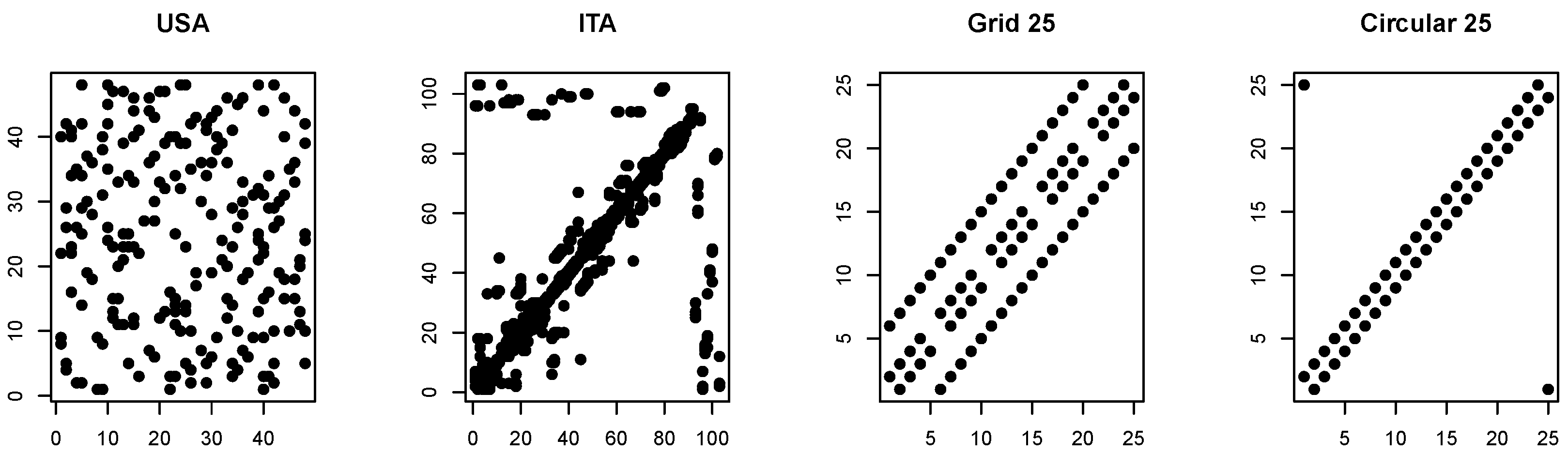N “closing” the circle. The corresponding neighborhood matrices are represented below in Figure 1. Notice that for the real-world cases, there is no natural ordering; in this instance, USA is alphabetical, while ITA is ordered by province code, running approximately northwest to southeast. Hence, the impression of a greater regularity, which breaks after the 92nd province (from the 93rd on, new provinces scattered across the country have been added in order of institution). (Needless to say, the ordering of the neighborhood matrix does not have any effect on the results, provided, of course, that it is correctly matched to that of the data.)

Synthetic orderings are generated for N of 25, 49, and 100; 49 instead of 50 because Grid needs N to be a perfect square. The corresponding densities (number of nonzero elements) are reported in

Table 2. Spatial contiguity structures and characteristics (dimensions and density of nonzero elements) of the corresponding binary neighborhood matrices.

Name	Description	N	Density
USA	Continental states of the USA	48	9.3
ITA	Provinces of Italy (between 1995 and 2005)	103	4.3
Grid	Regular “chess” grid, queen contiguity	25	12.8
		49	7.0
		100	3.6
Circular	Pesaran and Tosetti (2011) “circular world”	25	8.0
		49	4.1
		100	2.0

.

The above spatial orderings are supposed to be representative of a large share of applied practice. Circular and Grid, as I consider them here, are perhaps representative of the majority of “regular” orderings; although another one that might be considered is the so-called rook-type contiguity, whereby neighbors share a common border (but common vertices do not count). Conversely, there is almost an endless choice of “real-world” spatial orderings, but a coherent picture already emerges from the two very different geographies presented here. Moreover, the role of the USA and ITA in this paper is as a motivating example, delegating the structured inquiries to Circular and Grid.

3.2. Size-Power Graphs

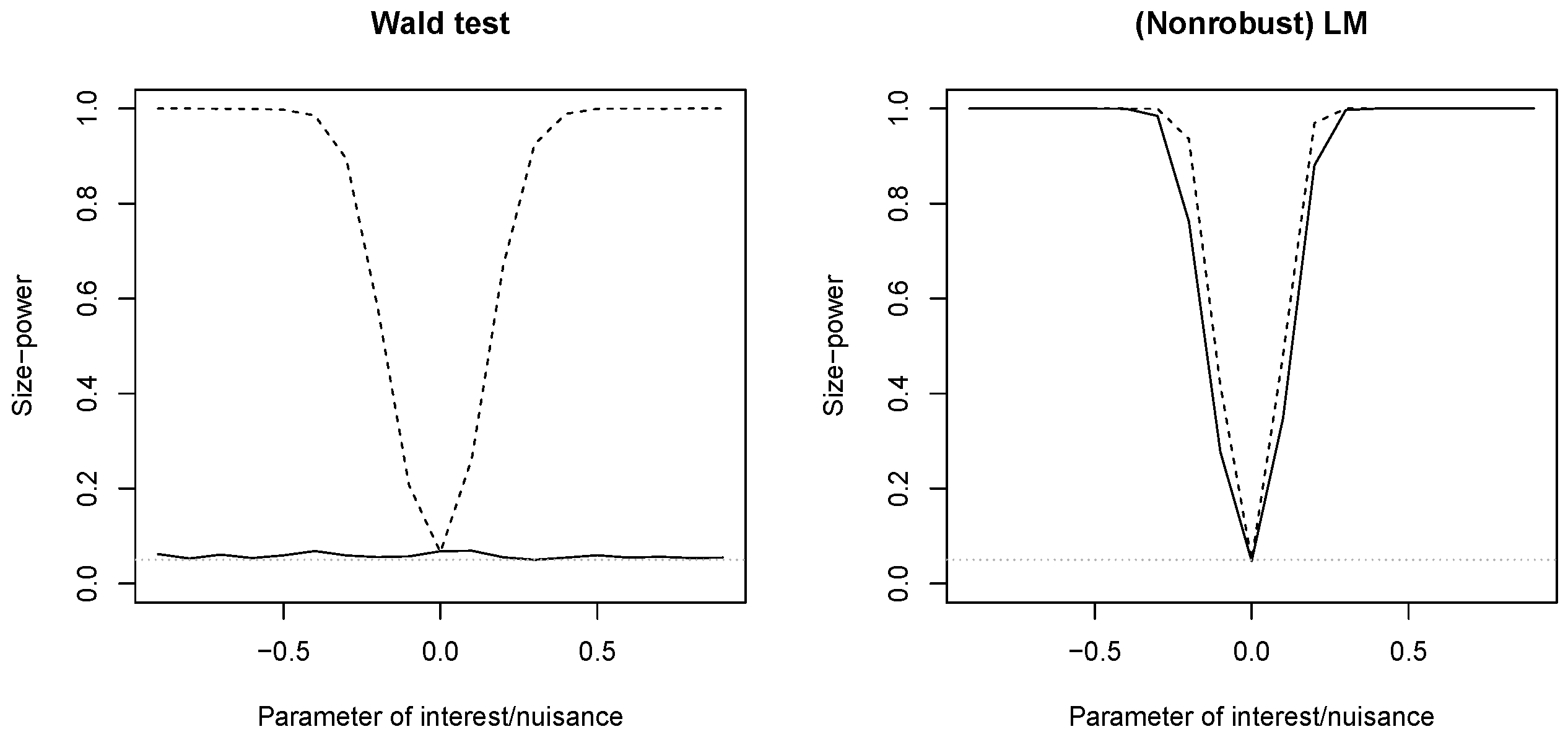
For compactness—and because what counts for specification purposes is the comparison between them—the results are presented through size-power graphs contrasting, in each setting, the performance of the pair of tests. Size-power graphs will be presented with respect to one spatial parameter (say, $\lambda$), changing from −0.9 to 0.9 in steps of 0.1, contrasting the behavior of the $RL{M}_{\lambda |\rho }$ test, which should ideally have an empirical rejection rate of about 5% at $\lambda =0$, to rise toward 1 “as fast as possible” as $\left|\lambda \right|$ grows (power), with the behavior of $RL{M}_{\rho |\lambda }$, which should instead remain close to the design size of 5% irrespective of $\lambda$ (robustness to the misspecified alternative). The distance between the power of the correctly specified test and the size of the “other” test measures the ability of the pair of RLM tests to give directions in the specification search (see Figure 2).

4. Monte Carlo Experiments

4.1. Experiment 1: Real World(s)

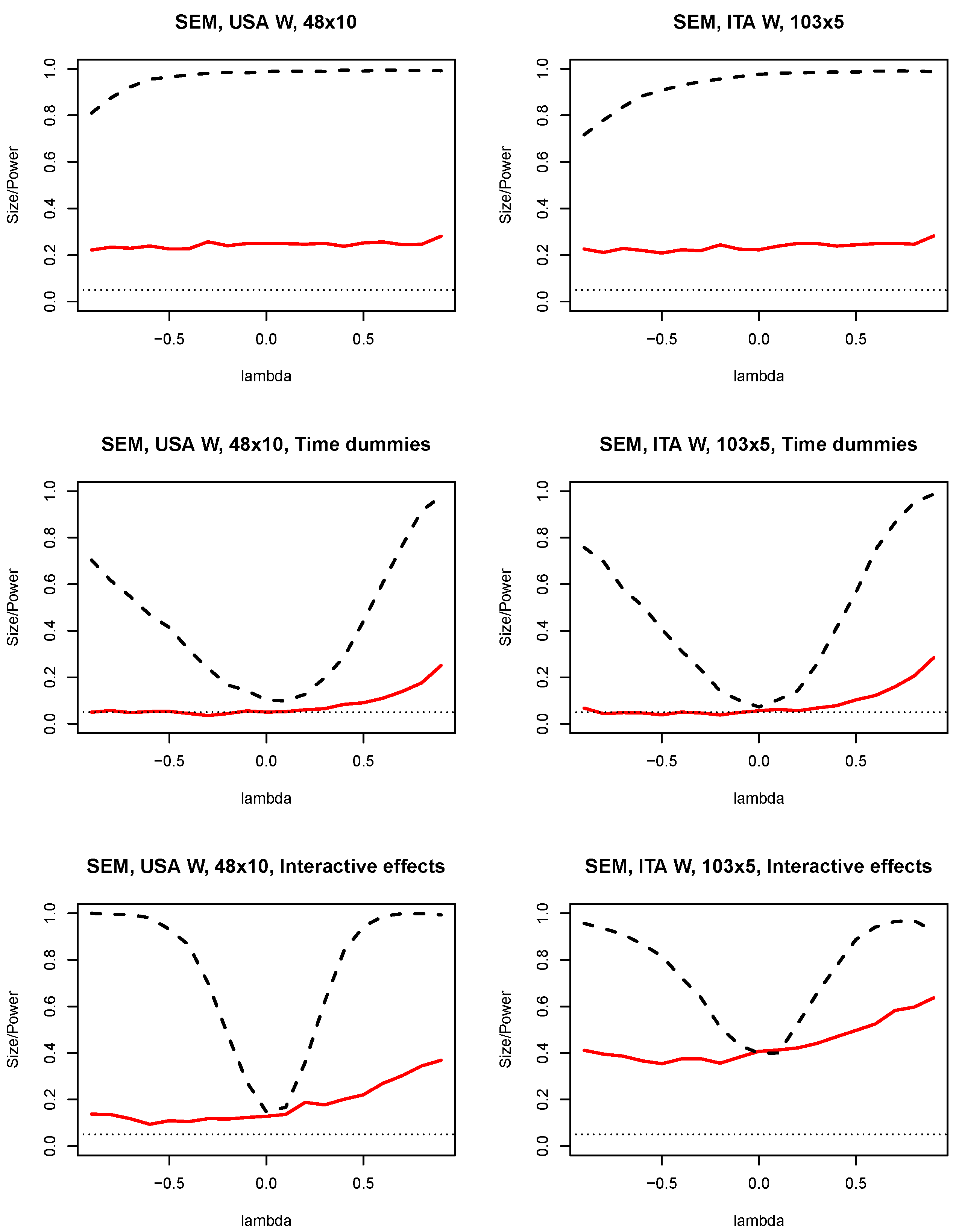
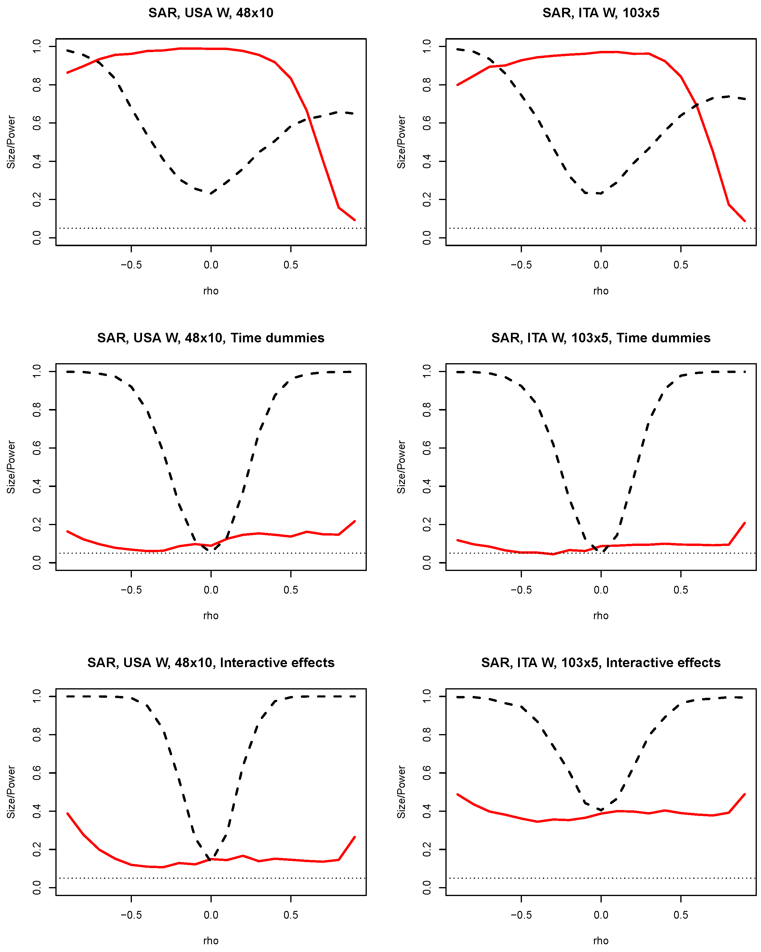
In the following figures, I compare the performance of three strategies in the face of time heterogeneity of the common-factor type: no augmentation, augmenting the test equation with time dummies (TFE), or with interactive fixed effects (IFE). Figure 3 is dedicated to the spatial error (SEM) scenario, Figure 4 to the spatial lag (SAR). This first experiment illustrates the perils of neglecting time heterogeneity: while the performance of augmented tests can range from basically useless to quite good in terms of size and power, they are always correctly centered; by contrast, those ignoring time heterogeneity, as already found by Millo [11], are—as expected—hopelessly biased.

First of all, it is clear that ignoring time heterogeneity of the common-factor type makes the RLM tests completely useless (first rows of Figure 3 and Figure 4). The reasons are similar to those of the homogeneous time effects cases addressed in (Millo [11], Experiment 4). Omitted common factors induce a cross-sectional correlation in model residuals, against which spatial diagnostics have power: hence, in the SEM case (Figure 3), the empirical power of $RL{M}_{\lambda |\rho }$ is biased toward rejection across the whole domain of $\lambda$, including $\lambda =0$; in turn, the empirical size of $RL{M}_{\rho |\lambda }$, although uniform, is much larger than the nominal size, at around 20%. In the SAR case (Figure 4), the correctly specified $RL{M}_{\rho |\lambda }$, although severely biased, maintains some power for positive $\left|\rho \right|$; but the empirical size of $RL{M}_{\lambda |\rho }$ veers totally off, so that the signaling value of the pair of tests is again zero (or negative, as here—at least, for $\left|\rho \right|\le 0.6$—a comparison would favor the opposite alternative to the “true” one!).

Time dummies augmentation (TFE, center rows of Figure 3 and Figure 4) does clearly help. The empirical size is taken down to acceptable values, somewhat irregularly (over-rejecting behavior for SEM with positive $\lambda$, slight over-rejection across the board for SAR), but these are common to the RLM tests in ideal conditions [10,11]. Power is modest (particularly so on the negative side) in the SEM case and rather good in the SAR case. Together with the acceptable size of the “misspecified” alternative, this makes the signaling value of the pair of RLM tests with time dummies rather good for specification purposes.

Adding interactive fixed effects (IFE) to the RLM test equation would be expected to improve test performance, as fully estimating out the influence of the common factors should yield residuals “clean” of any unwanted non-spatial dependence, improving test power and correcting test size. In practice, these expectations are only partly fulfilled, while a further problem emerges, particularly acute in the short panel case (ITA).

Indeed, in the SEM/USA scenario, IFE markedly improves the power of the RLM test with respect to TFE (compare the second and third items of the first column in Figure 3). Power rises toward 1 for $\left|\lambda \right|=0.5$, which is comparatively good for such a small sample size, although the empirical size shows a rather large bias. In the “short panel” ITA case, under the SEM scenario, the comparison between IFE and TFE reduces to the choice between a correctly sized but underpowered test and one where the empirical size—both for the correctly specified and the misspecified test—is ten times the nominal level (see the second and third items of the first column in Figure 3).

In the SAR scenario (Figure 4), the properties of TFE-augmented RLM tests are good, especially in the “short panel” ITA case: time dummies seem to be enough to account for time heterogeneity, even under common factors with heterogeneous loadings. By contrast, there is little to be gained from IFE in terms of power, but much to be lost in terms of size bias, again substantial for the USA and unacceptably high for ITA (compare the second and third rows of Figure 4, and in particular the rightmost elements).

Thus, from these tentative simulations reproducing potential real-world cases, one gets the impression that IFE introduces a tradeoff between improved power and biased empirical size, and that this tradeoff is particularly severe for very short panel datasets. This is broadly consistent with the a priori expectation that the large number of estimated incidental parameters from IFE (which grows with $NT$) introduces uncertainty that is not accounted for by the RLM procedure, inflating empirical size; it also suggests that this effect may be asymmetric and inversely related to the time dimension, or perhaps to the ratio $T/N$.

In the following, I try to reproduce the above behavior in a systematic way in order to infer regularities and, hence, to give directions for applied practice.

4.2. Experiment 2: Synthetic Spatial Structures

Next, I try to assess the behavior of IFE vs. TFE for different combinations of N and T in a structured way, in order to possibly infer regularities and hence give directions for applied practice. To this end, I employ the synthetic spatial structures presented above, Grid and Circular, expanded along different cross-sectional dimensions.

In this second experiment, I changed the visualization of results. It has been established that the no-augmentation strategy is not viable; therefore, the results are omitted. I would rather concentrate on the comparison between TFE and IFE, representing them together in each “small multiple” graph, so as to give an immediate impression of the evolution of their empirical properties as N grows (rows, left to right), as T does (top to bottom), or as they grow together (diagonal).

As it turns out, despite the very different spatial orderings, the results are largely comparable. Therefore, in the following, I only present the results for Grid; those for Circular are to be found in the Appendix A. I do not report non-augmented RLM tests, which are hopelessly biased in any of the experiments and across any scenario and combination of parameters, concentrating instead on the comparison between TFE and IFE.

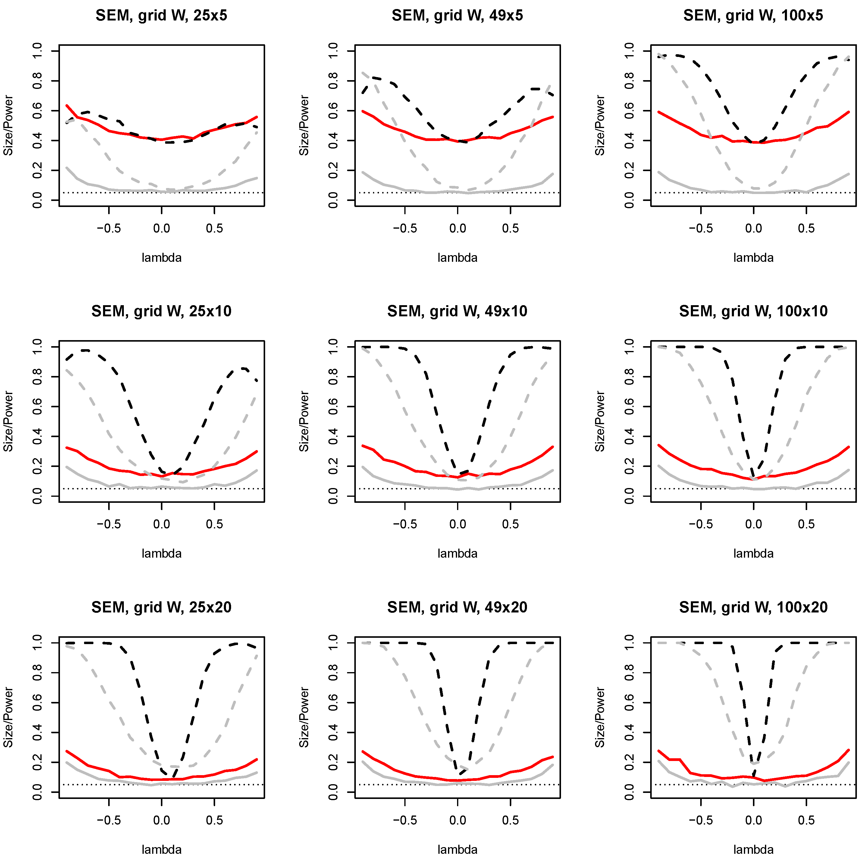
4.2.1. Comment: SEM Scenarios

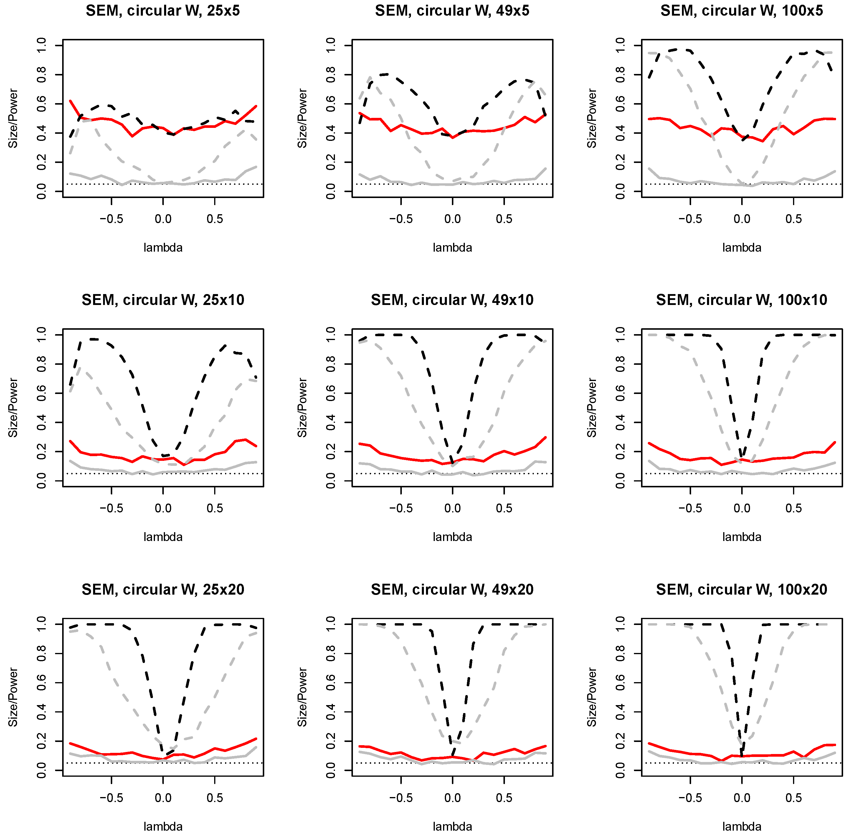
Spatial error (SEM) scenarios in either space, Grid (Figure 5) or Circular (Figure A1), yield largely similar results. For $T=5$, IFE is unacceptably—and uniformly—over-rejecting across any N; TFE is instead correctly sized, and power for all tests increases with N, from too low to be of any practical help when $N\le 50$ toward “usable” levels when $N=100$.

The IFE strategy starts to prevail for $T=10$, yielding much better power properties if one is prepared to put up with empirical sizes approaching 20%. When $T=20$, over-rejection of IFE becomes rather mild, while power is very good even for the “small” panel at $N=25$, where TFE has low power. As the sample size grows, both IFE and TFE are viable specification devices under SEM (bottom right panels of Figure 5 and Figure A1).

4.2.2. Comment: SAR Scenarios

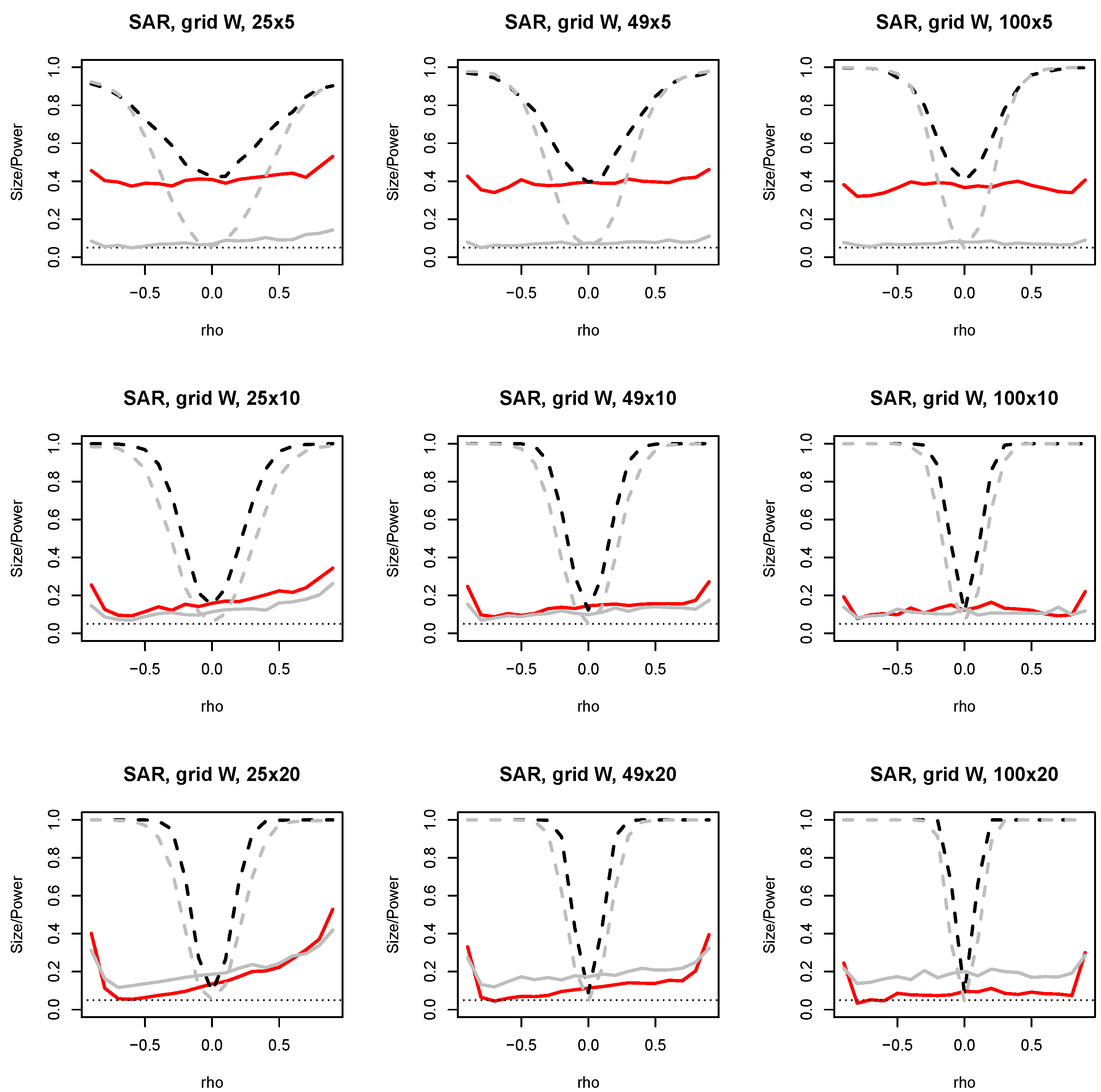
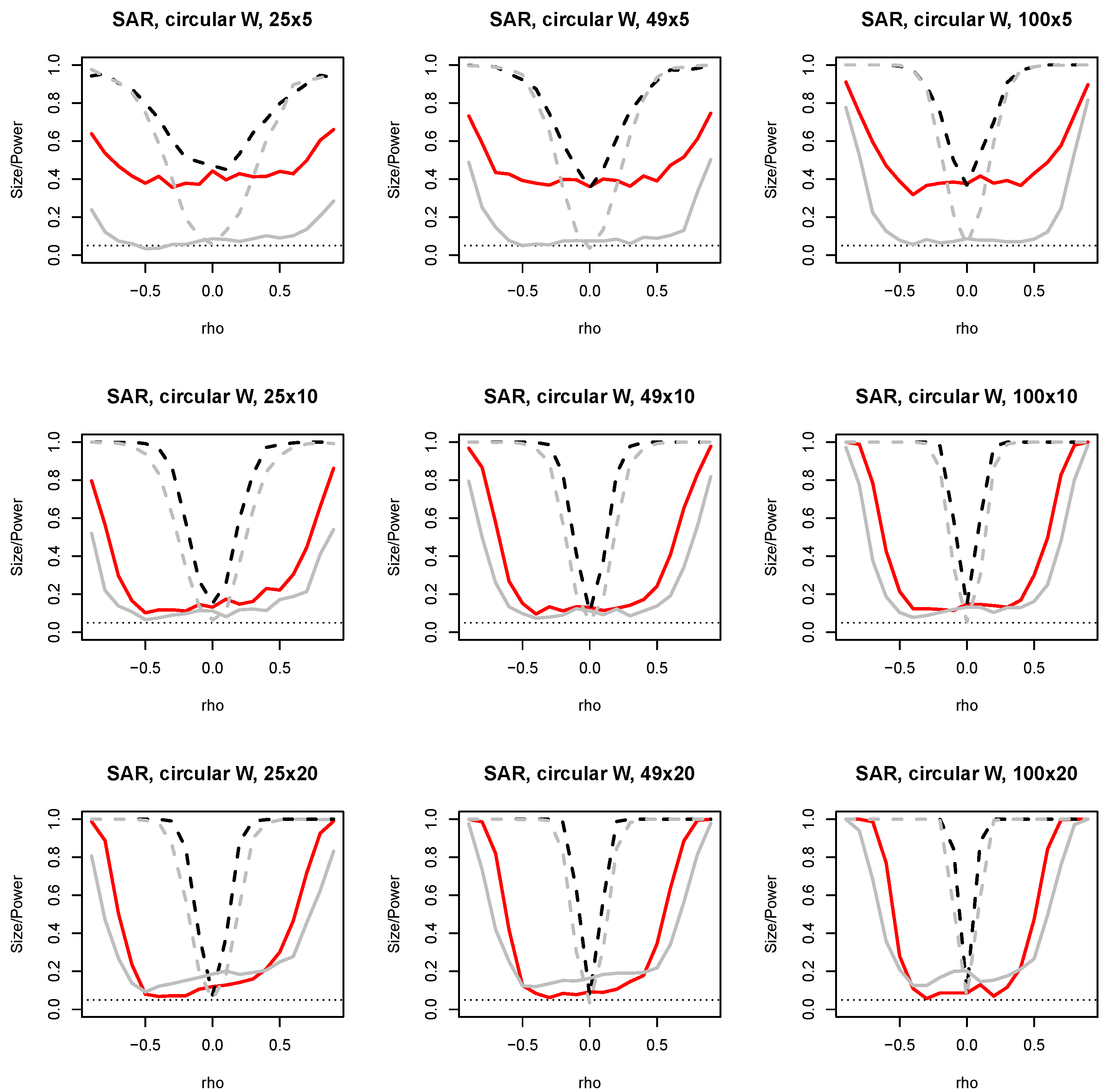
Spatial lag (SAR) scenarios in either space are reported, respectively, in Figure 6 (Grid) or Figure A2 (Circular). Again, for $T=5$, IFE is unacceptably over-rejecting while TFE is correctly sized, irrespective of N; but this behavior quickly fades away as T exceeds 10. Test power improves with N again, but here the power of TFE is much closer to that of IFE.

An empirical peculiarity of $RL{M}_{\lambda |\rho }$, already observable from previous simulation work, is the tendency of empirical test size under the “other” alternative (here, red solid lines) to diverge toward each end of the nuisance parameter space (i.e., for $\left|\rho \right|$ increasing toward 1). This feature, which becomes more prominent with both growing T and N, is clearly dependent on the spatial context, being apparent only for extreme values of $\left|\rho \right|$ under the Grid space, while under the Circular arrangement it kicks in dangerously early. In fact, in the latter case, the size of $RL{M}_{\lambda |\rho }$ can diverge toward one as early as $\left|\rho \right|=0.6-0.7$ when $N=100,T=20$ (Figure A2, bottom right panel).

On the other hand, the empirical size of $RL{M}_{\lambda |\rho }$ can be seen to increase gradually away from $0.05$ for positive values of $\rho$, this time irrespective of the spatial ordering. This tendency becomes worse with increasing T and is clearly mitigated by increasing N: in other words, empirical size is distorted toward over-rejection for positive $\rho$ as $T/N$ grows larger.

4.2.3. Summary and Takeaways for Applied Practice

Disregarding time effects altogether is always a bad idea, and under common factors, both IFE and TFE augmentations will provide a valid correction to the tests for any sample size but the very smallest ones. As regards the behavior of TFE vs. IFE, the results are nuanced. While in principle IFE would seem the ideal strategy, in practice the above-mentioned incidental parameter problem induces a bias in the test size, which is clearly evident and of unacceptable magnitude in the $103\times 5$ cases; on the other hand, the suboptimal TFE correction clearly yields tests with lower power across the board. Problems are mostly confined to smaller sample sizes, some unrealistically small ($25\times 5$), while from $50\times 10$ on, the properties of the tests start to be acceptable, with behavior getting proportionally better as samples grow large. The only exception to this rule is the pathologies of empirical size at large values of the nuisance parameter, which can be more extreme under some spatial orderings (here: Circular, SAR scenario) and seem to be exacerbated by the IFE augmentation. Nevertheless, these issues are already well known from the previous literature, and it must be noted that from the beginning, the locally robust RLM tests were not designed to work in these regions of the parameter space.

One could tentatively conclude that it is “safe” to go with IFE for time dimensions of $T>10$, especially if approaching $T=20$ (which includes “long panel” studies in the common-factor literature in particular, and in general, the best part of empirical spatial panel work). Very short panel studies (say, $T<10$) will require TFE, which is always satisfactorily sized but becomes dependable in terms of power for T approaching 100 (or even 50, for the SAR case). Although heterogeneous time dependence is a possibility regardless of sample size, for practical reasons, researchers will seldom approach very short panels from a common-factor perspective.

5. Discussion, Limitations, and Directions for Future Research

The simulations presented here are based on a limited number of spatial orderings and sample sizes: although the former are quite typical of standard practice in terms of ordering and density, and the latter should be representative of the most problematic cases (very small samples in space and/or time). Experimentation across different spatial matrices and different densities of the same ones (e.g., obtained by increasing the order of spatial neighborhood beyond 1) might yield different results.

Crucially, a single structure is considered for the heterogeneous factor loadings: uniform sampling between 0 and 2. Different choices are possible (a sensible one, also in terms of comparison with time fixed effects, which have identically 1 loadings, would be sampling between −1 and 1). Again, in principle, results might differ from the ones presented here, especially for the TFE strategy (under IFE, the effect of common factors is estimated out).

It must also be noted that the results presented here are specific to some spatial orderings, albeit quite representative of current practice; robustness checks with alternative geographies have yielded consistent findings, but the context dependence of RLM tests (see Figure 2 and, in particular, Experiment 6 in [11]) still requires caution.

Nevertheless, the present note is not meant as an exhaustive description of test properties across potential scenarios—a close to impossible task, given the wealth of possible cases, or at least a computationally very expensive one—but as a counterexample and an illustration of problematic outcomes. It aims at signaling eventual problems, some of which are evident from the outcomes presented above. Between the potential scenarios a spatial panel data analyst can encounter while addressing the “lag vs. error” specification issue, the common factors case stands out as requiring a more cautious approach, although problems seem to be confined to very small samples.

6. Conclusions

This paper aims to assess the viability of a specification strategy for the spatial process in spatial panels characterized by unobserved common factors, based on augmenting the test model with interactive fixed effects, analogous to the fixed effects augmentation strategy proposed in Millo [11]. In this paper, I only provide intuition and simulation evidence, leaving an analytical investigation of the size bias for future work. In any case, some findings that could be expected based on extant literature do stand out without much doubt, showing some clear indications for applied practice.

Unfortunately, unlike the homogeneous time fixed effects case, where an augmentation strategy can always preserve the good properties of the RLM tests, in the case of common factors with heterogeneous loadings, the first-best strategy of augmenting the test equation with interactive fixed effects finds a natural limit in the large number of incidental parameters it would introduce. On the other hand, in the presence of heterogeneous factor loadings, TFE—which does not share this weakness—would be a second-best strategy, and is shown here to suffer potentially large power losses. I therefore end up comparing two suboptimal strategies for controlling for time heterogeneity: time fixed effects (TFE) against interactive fixed effects (IFE). While not controlling is always a bad idea in the potential presence of time heterogeneity, leading to severely biased and practically useless RLM statistics, both TFE and IFE do recenter the test statistics, restoring some signaling value: how much depends on the sample sizes N and T.

While IFE is uniformly more powerful across all my experiments, the size bias becomes unacceptably large, sometimes approaching 40%, for short panels (here represented by $T=5$). Conversely, TFE is usually better sized but can suffer a loss of power so large as to leave little signaling value. In some situations, a researcher may therefore be better off controlling for the unobserved time heterogeneity in test equations by simple time dummies than by adding interactive fixed effects. The above results suggest that TFE is a safer bet in the case of very short panels. For moderately sized samples, and in particular when $T>10$, IFE becomes preferable, although over-rejection issues can be present until $T>20$.

Summing up, this paper has addressed the specification of spatial processes of the spatial autoregressive vs. spatial error type in panel data by means of the robust Lagrange multiplier tests of Anselin et al. [10], from the point of view of a researcher who is agnostic as regards the further “typical panel” features of the data-generating process, in particular, as regards the presence of (potentially correlated) time heterogeneity of homogeneous (time fixed effects) or heterogeneous nature (common factors). While an agnostic approach—based on generic augmentation of the test equation—has been shown to work well against other features like individual heterogeneity and serial correlation [11], in the case here presented, the side effects of IFE augmentation on test properties (in particular, empirical size) can be severe. In turn, the simpler TFE strategy can be more robust in terms of size but lacks power. Neither is as dependable across different sample sizes as in the case of individual or time effects with homogeneous loadings. Still, either one tends to work acceptably well for the most common sample sizes or larger, and either is much preferable to simply ignoring time effects, as is done in a large part of the applied literature (see Table 1 in [11]).