How to Find the Covering Radius of Linear Codes over Finite Fields Using a Parity-Check Matrix in Parallel

Abstract

We present a parallel algorithm for computing the covering radius of a linear ${[n,k]}_q$ code using its parity-check matrix. The method is based on the systematic generation of syndromes associated with linear combinations of columns of the parity-check matrix. To improve scalability, the search space is partitioned and processed in parallel using a master–worker strategy implemented with the Message Passing Interface (MPI). The proposed approach significantly reduces the computational effort required for covering radius computation, a problem known to be NP-hard in general. Experimental results demonstrate that the parallelization achieves substantial speedups and makes the exact computation of the covering radius feasible for codes of larger parameters.

1. Introduction

In coding theory, linear codes are used to detect and correct errors in transmitted messages over noisy channels. A linear ${[n,k]}_q$ code C over a finite field ${\mathbb{F}}_q$ is a k-dimensional subspace of the vector space ${\mathbb{F}}_q^n$, consisting of $q^k$ codewords. Key parameters of a code include its length n, dimension k, and minimum distance d. With each linear code C, we associate two matrices: generator and parity-check matrix. A matrix G with k rows and n columns is called a generator matrix of a linear code C if the rows of G form a basis of C. An $(n-k)\times n$ matrix H, such that $C=\{c\in {\mathbb{F}}_q^n:H{c}^T=\mathbf{0}\}$, is called a parity-check matrix for C.

Let us consider the full vector space ${\mathbb{F}}_q^n$. It is partitioned into a disjoint subsets of the form $v+C=\{v+c:c\in C\},$ where $v\in {\mathbb{F}}_q^n$. These subsets are called cosets of the linear code C. For any vector $v\in {\mathbb{F}}_q^n$, we define its syndrome as $\mathrm{syn}\left(v\right)=H{v}^T$. There is a one-to-one correspondence between cosets of C and syndrome vectors in ${\mathbb{F}}_q^{n-k}$.

The covering radius R of a linear code C is defined as

$$R=\underset{v\in {\mathbb{F}}_q^n}{max}\underset{c\in C}{min}{d}_H(v,c),$$

i.e., the smallest integer such that every vector in the vector space lies within Hamming distance R of some codeword. The covering radius R can be interpreted as the minimal number of columns of H whose linear combinations generate all syndromes.

The covering radius is a classical and fundamental parameter in coding theory. While the minimum distance d quantifies the error-correction and error-detection capabilities of a code, the covering radius R measures how well the code covers the ambient space and provides complementary information about the global geometry of the code. In classical error detection, the minimum distance d guarantees that any error pattern of weight less than d can be detected. However, in the general decoding and detection setting, the received word may be arbitrary and not necessarily close to a valid codeword. In this broader context, the covering radius plays a crucial role. A small covering radius guarantees that every received word lies within a bounded distance from the code, which implies that undetectable error patterns are confined to well-structured regions of the ambient space.

In erasure channels, some symbols of a transmitted codeword are erased, while the remaining symbols are received correctly [1]. Decoding from erasures amounts to determining whether the known positions uniquely determine a codeword. A small covering radius guarantees that every received word, including those resulting from erasures, is close to at least one codeword. Moreover, the covering radius is directly connected to the structure of coset leaders and syndrome decoding, which are fundamental tools in erasure recovery for linear codes.

Locally recoverable codes (LRCs) have received significant attention due to their applications in distributed storage systems [2]. An LRC is a code in which each coordinate can be recovered by accessing only a small number of other coordinates. Although locality is a coordinate-wise property and the covering radius is a global parameter, there exists a strong conceptual connection between the two. Codes with small covering radius induce highly regular partitions of the ambient space. Such structural properties are closely related to the existence of multiple recovery sets for individual symbols, which is a key requirement in the construction of locally recoverable codes.

Covering radius plays a central role in several other areas: lossy compression and vector quantization [3], in certain information-hiding schemes [4]. Codes with small covering radius often exhibit strong symmetry and regularity properties, such as complete regularity or uniform packing, which are of independent combinatorial interest [5].

Despite its importance, computing the covering radius is known to be NP-hard. This makes the development of efficient algorithms, and in particular parallel algorithms, highly relevant both theoretically and practically. Efficient computation of the covering radius enables structural analysis of codes used in distributed storage and data protection, exploration of new code families with strong geometric and spectral properties. Therefore, improving the computational feasibility of determining the covering radius directly supports both the theory and the practice of modern coding techniques.

There are different methods for calculating the covering radius of a linear ${[n,k]}_q$ code. One algorithm is based on the definition. The naive approach is to compute the distance from each vector to the code C. Another method uses the parity-check matrix of the code and is based on Lemma 1.1 from [6]. The covering radius can also be calculated using fast transforms [7]. Some results on the problem of computing the covering radius can be found in [8,9,10,11,12]. Specialized techniques can be used to calculate the covering radius of some classes of codes such as MDS and near MDS codes [13,14], Melas codes [15], Zetterberg codes [16,17], etc. Heuristic and probabilistic methods can also be used. However, they do not give us an exact value for R.

We present a method to parallelize the algorithm for computing the exact covering radius of a linear code using its parity-check matrix. This problem is at least as complex as the problem for computing the minimum distance of a code. Parallel algorithms for computing the minimum distance of a binary code are presented in [18,19]. On the other hand, this work is a continuation of a previously developed parallelization of the algorithm for calculating the covering radius using cosets of the code. A disadvantage of that algorithm is that we generate the full vector space $F_q^n$ to compute the covering radius. The considered algorithm in this paper only keeps track of generated $F_q^{n-k}$ syndromes, which however requires a larger amount of memory. This algorithm is more appropriate to be used for codes with larger dimensions. For any parallel implementation, we need to use an optimized sequential algorithm. The basis of the algorithm is the systematic generation of vectors in ${\mathbb{F}}_q^{n-k}$ by forming linear combinations using l columns of the matrix H, where l increases ($l=1,2,\dots$). Each linear combination of l columns of H can be represented as an n-dimensional vector with weight l. Thus, the algorithm can be represented as generating all vectors $v\in {\mathbb{F}}_q^n$ with $wt\left(v\right)\le l$. There are different approaches to generate all vectors in a given set. In the case when $l=n$, we can use a Gray code for the generation. When $l<n$, the classical Gray code cannot be used directly, and therefore some modifications are needed. In this case, a linear combination can be generated by adding and subtracting a vector from the previous linear combination. Here, we have two operations to generate a linear combination. Another approach is to use a helper matrix that contains a linear combination of s columns of H in row s. Using such matrix, we can generate the next linear combination by using just addition at the expense of greater memory complexity. Such an algorithm is less researched compared to the Gray code methods. This is the most efficient method for generating linear combinations, as far as we know. We also need to keep track of the already generated linear combinations which correspond to syndromes for the given code in order to calculate the covering radius. If for a given l all ${\mathbb{F}}_q^{n-k}$ syndromes are generated as a linear combination of not more than l columns of H, then $R=l$ is the covering radius of the code.

The focus of the current work consists of an in-depth view of the following problems:

• Defining an ordering of the vectors $v\in {\mathbb{F}}_q^n$ with $wt\left(v\right)\le l$ that correspond to a linear combination of the columns of the parity-check matrix H of a linear ${[n,k]}_q$ code C. In the chosen order, a new linear combination is generated by just adding a vector to a previous linear combination. Furthermore, each vector in the ordering is generated efficiently.
• Presenting ranking and unranking algorithms for the given ordering. A ranking function assigns an integer to a given combinatorial object in a chosen ordering. The inverse function that gives the combinatorial object in a specific ordering for a given valid integer (rank) is called unranking function. Such algorithms are typically defined for basic combinatorial objects.
• Efficiently partitioning the vectors in the given order into subsets such that the vectors in each subset follow the same order and all subsets have approximately the same cardinality.
• Efficient enumeration of the vectors in ${\mathbb{F}}_q^{n-k}$ that correspond to the syndromes for the code.

A key conceptual contribution of this work is the introduction of explicit ranking and unranking functions for the combinatorial objects underlying the covering radius computation. Unlike classical combinatorial generation methods, which rely on sequential or backtracking-based enumeration, ranking and unranking provide a direct bijection between integers and linear combinations of columns of the parity-check matrix. This representation fundamentally changes the algorithmic structure by allowing random access to the search space and enabling its deterministic partitioning into independent subspaces. As a result, the use of ranking and unranking functions is essential for an efficient parallel implementation, since without them a balanced distribution of work among worker processes would not be feasible.

The Message Passing Interface (MPI) was chosen as the parallelization framework for several reasons. First, MPI is a widely adopted standard that provides portability and scalability across a broad range of computing architectures, from multicore systems to large distributed clusters. Second, the explicit data distribution model of MPI allows for an efficient integration of low-level optimizations, such as vectorization, within each process, without interfering with the global parallel structure. Finally, the sequential covering radius algorithm naturally follows a master–worker paradigm, where a central process coordinates the exploration of the syndrome space and multiple workers perform independent computations. This execution model is straightforward to implement in a message-passing environment, while it is considerably more difficult to realize efficiently in shared-memory parallel frameworks.

The remainder of the paper is organized as follows. Section 2 introduces the necessary definitions and preliminaries. An overview of the parallel frameworks considered in this work is provided in Section 3. The sequential algorithms are described in Section 4, followed by their parallelization strategies in Section 5. Experimental results and performance evaluation are presented in Section 6. Finally, Section 7 concludes the paper with a summary and concluding remarks.

2. Preliminaries

Let ${\mathbb{F}}_q$ be a finite field with q elements, and let C be an $[n,k]$ linear code over ${\mathbb{F}}_q$. The minimum distance d measures the smallest Hamming distance between distinct codewords:

$$d=\underset{c_1\ne c_2\in C}{min}{d}_H(c_1,c_2),$$

where $d_H(·,·)$ denotes the Hamming distance. The minimum distance is one of the most searched parameters of a linear code. It shows how many errors a code can detect or correct. More precisely, a linear $[n,k,d]$ code can detect up to $d-1$ errors and correct up to $\lfloor (d-1)/2\rfloor$ errors. Another important parameter of the code, that gives additional information, is its covering radius. The covering radius R of a code C is defined as

$$R=\underset{v\in {\mathbb{F}}_q^n}{max}\underset{c\in C}{min}{d}_H(v,c),$$

Equivalently, R is the smallest integer such that the Hamming spheres with radius R centered at the codewords cover the entire space ${\mathbb{F}}_q^n$.

The covering radius of a linear code can be computed using its parity-check matrix or coset leaders. Let $C^{\perp }$ denote the dual code of C, defined as

$$C^{\perp }=\{u\in {\mathbb{F}}_q^n|\langle u,c\rangle =0\mathrm{for}\mathrm{all}c\in C\},$$

where $\langle ·,·\rangle$ is the standard inner product over ${\mathbb{F}}_q$. The dual code has parameters ${[n,n-k]}_q$. The generator matrix of $C^{\perp }$ is the parity-check matrix of C such that

$$C=\{v\in {\mathbb{F}}_q^n:H{v}^{\top }=0\}.$$

If $v\in {\mathbb{F}}_q^n$ then the set

$$\mathbf{v}+C=\{\mathbf{v}+\mathbf{c}:\mathbf{c}\in C\},$$

is called a coset of C represented by v. The vector space ${\mathbb{F}}_q^n$ can be partitioned into disjoint cosets, and two vectors ${\mathbf{v}}_1$ and ${\mathbf{v}}_2$ are in the same coset if and only if their difference belongs to C, i.e., ${\mathbf{v}}_1-{\mathbf{v}}_2\in C$. A vector of minimum weight within a given coset is called a coset leader.

For any vector $\mathbf{v}\in {\mathbb{F}}_q^n$, we define its syndrome as

$$\mathrm{syn}\left(\mathbf{v}\right)=H{\mathbf{v}}^T.$$

Syndromes provide an algebraic characterization of cosets: two vectors belong to the same coset of C if and only if they have the same syndromes. Thus, there is a one-to-one correspondence between cosets of C and syndrome vectors in ${\mathbb{F}}_q^{n-k}$. Hence, the syndrome completely identifies the coset to which a vector belongs.

The following theorem gives the connection between the covering radius, parity-check matrix and code leaders of a given linear code C.

Theorem 1 

([20]). Let C be a linear code with a parity check matrix H. Then,

(i) 

$R\left(C\right)$  is the weight of the coset of largest weight;

(ii) 

$R\left(C\right)$ is the smallest number s such that every nonzero syndrome is a combination of s or fewer columns of H, and some syndromes require s columns.

Several methods are known for determining the covering radius of a linear code. One approach is based directly on the above theorem, requiring the identification of all coset leaders and their weights. Since there is a one-to-one correspondence between cosets and syndromes, we can also consider an algorithms that generates all syndromes. The covering radius is also interpreted as the smallest integer R such that all $(n-k)$-dimensional vectors (syndromes) can be represented as linear combinations of no more than R columns of a chosen parity-check matrix H of the code. In other words, we need to generate the full vector space ${\mathbb{F}}_q^{n-k}$, which is a computationally heavy problem. Thus, we can also consider a lower bound for R.

The volume of the ball within a q-ary Hamming sphere of radius r in ${\mathbb{F}}_q^n$ is

$$S_q\left(r\right)=\sum _{i=0}^r\left({\displaystyle \genfrac{}{}{0pt}{}{n}{i}}\right){(q-1)}^i.$$

This counts the number of vectors within the distance r of a given center. The union of spheres of radius R centered at each codeword must cover all vectors in ${\mathbb{F}}_q^n$. Thus,

$$q^k{S}_q\left(R\right)\ge q^n,$$

which can be rearranged to give

$$S_q\left(R\right)\ge q^{n-k}.$$

Consequently, the covering radius satisfies the combinatorial lower bound

$$R\ge R_{min},R_{min}=min\left\{r\in \mathbb{N}:S_q\left(r\right)\ge q^{n-k}\right\}.$$

If $R=\lfloor (d-1)/2\rfloor$, the code is called a perfect code. For the perfect codes $q^k{S}_q\left(R\right)=q^n$. This lower bound is called Sphere Covering Bound and is also given in [8].

3. Parallel Computing Framework and Vectorization

The Message Passing Interface (MPI) is the de facto standard for parallel computing in distributed-memory environments. Unlike shared-memory models, MPI provides explicit communication primitives that allow processes to exchange data through messages. This design enables programs to scale efficiently across clusters, supercomputers, and heterogeneous systems where each processing unit has its own private memory space. More on parallel programming with MPI can be found in [21].

Vectorization, on the other hand, provides mechanisms for additional parallelization in algorithms that include vector operations. The main idea of vectorization is to execute an operation over multiple elements of the vector at the same time. This can be accomplished by utilizing extended vector registers that are available in most modern central processing units (CPUs). Vectorization with such registers can be used in combination with other parallel mechanisms and standards such as MPI.

3.1. MPI: The Master–Worker Paradigm

MPI programs follow the Single Program Multiple Data (SPMD) execution model: all processes execute the same program but operate on different portions of the data. Communication is performed through point-to-point or collective operations, such as MPI_Send, MPI_Recv, MPI_Bcast, and MPI_Reduce. This explicit communication model offers fine-grained control over performance and resource usage, making MPI suitable for complex, large-scale scientific computations.

A widely used pattern in MPI applications is the master–worker paradigm. In this model, one process (the master) coordinates the computation, while the remaining processes (the workers) perform the actual computational tasks. The master is responsible for distributing work units, collecting results, and determining global termination conditions. The workers repeatedly receive tasks from the master, execute them independently, and return results.

This paradigm is especially beneficial for applications where the workload is irregular or dynamically generated. It allows the master to balance the load by assigning tasks adaptively, preventing situations where some processes remain idle while others are overburdened. The flexibility of task granularity enables the programmer to tune the communication-to-computation ratio according to the characteristics of the problem and the underlying hardware. Such strategy can be used for different problems such as the classification of combinatorial objects [22].

MPI supports multiple communication strategies within master–worker systems. Tasks and results may be exchanged using blocking or non-blocking point-to-point communication (MPI_Isend/MPI_Irecv), allowing both the master and workers to overlap computation with communication. Collective operations may be used for global broadcasts (e.g., to distribute shared parameters) or reductions (e.g., to aggregate partial results), although the master–worker pattern often favors point-to-point interactions to minimize synchronization overhead.

3.1.1. Advantages

The master–worker paradigm offers several advantages in distributed-memory systems:

• Scalability: Since workers operate independently, the computation can scale to hundreds or thousands of processes with minimal contention.
• Dynamic load balancing: The master can adjust the distribution of tasks at runtime, leading to improved utilization of computational resources.
• Fault isolation: Errors are often confined to individual workers, and the master can detect failures or timeouts.
• Simplicity of design: The structure of the algorithm becomes modular, separating coordination from computation.

3.1.2. Limitations

Despite its advantages, the master–worker model also presents challenges:

• Master bottleneck: If the rate of task generation or result collection is high, the master may become a performance bottleneck.
• Communication overhead: Fine-grained task distribution may lead to excessive message traffic unless carefully optimized.
• Centralized control: The model relies on a single point of coordination, which may limit fault tolerance and scalability in extremely large systems.

3.2. Vectorization with Extended Vector Registers

An essential component of the proposed parallel procedure for computing the covering radius of linear codes over finite prime fields ${\mathbb{F}}_q$, with $q\le 64$, is the rapid evaluation of linear combinations of columns of a given parity-check matrix H. For a column vector $h\in {\mathbb{F}}_q^m$ and a partial sum $s\in {\mathbb{F}}_q^m$, the update

$$s\leftarrow s+h(modq)$$

is performed repeatedly within the enumeration process. Since all field elements can be represented in a single byte, the operation can be carried out efficiently via byte-wise modular addition within SIMD registers.

In the implementation, each column of H is packed into a 128-bit register, allowing the simultaneous processing of 16 coordinates. Modular addition in ${\mathbb{F}}_q$ is realized through a fixed sequence of SIMD operations involving byte-wise addition, comparison against the modulus, construction of a correction mask, and a selective blend to enforce reduction modulo q. Formally, letting $a,b\in {\{0,\dots ,q-1\}}^m$ denote the byte-encoded vectors, the register-level computation implements

$$a\oplus b=a+b-q·{\mathbf{1}}_{\{a+b\ge q\}},$$

where all operations are evaluated componentwise and ${\mathbf{1}}_{\{·\}}$ is realized via SIMD comparison and mask selection. This avoids lookup-based techniques and ensures that the entire update remains vectorized. Some algorithms for vector operations using vectorization with registers are presented in [23,24].

The use of 128-bit SIMD instructions markedly reduces the number of scalar iterations required in conventional implementations. Since an entire column vector fits within a single register, memory traffic is minimal, and repeated access to the same columns during the algorithmic search incurs negligible overhead. The resulting instruction sequence is short, uniform across fields with $q\le 64$, and well suited to superscalar execution.

Consequently, the SIMD-enhanced implementation achieves a substantial speedup in the evaluation of the linear combinations that dominate the computational complexity. These optimizations preserve exact arithmetic over ${\mathbb{F}}_q$ while allowing the algorithm to scale to parity-check matrices of nontrivial size and to explore significantly larger search spaces within practical time bounds.

Although wider SIMD extensions such as AVX2 and AVX–512 are available, they were not used in this work due to the interaction between vectorization and process-level parallelism. The proposed algorithm employs a large number of concurrent MPI worker processes, and on many architectures wider SIMD instructions lead to increased instruction latency and reduced core frequency, which can negatively affect overall throughput. Moreover, the computational kernel naturally fits into 128-bit registers, so wider SIMD registers do not significantly reduce the instruction count. For these reasons, SSE4.1 provides a balanced and portable solution, and a comparison with wider SIMD extensions was not pursued.

4. Sequential Algorithm

Let C be a linear ${[n,k]}_q$ code with parity-check matrix $H\in {\mathbb{F}}_q^{(n-k)\times n}$. Each syndrome $syn\left(v\right)=s,$ where $s\in {\mathbb{F}}_q^{n-k}$ corresponds to a coset of C in ${\mathbb{F}}_q^n$. By Theorem 1, the covering radius is the maximal weight of a coset leader, which is equal to the minimal number of columns of H whose linear combinations generate a syndrome. Thus, a syndrome is defined by a vector v, which corresponds to a linear combination of the columns of H. This gives us a direct algorithm to calculate the covering radius. Furthermore, from the sphere covering bound, we already know a lower bound $R_{min}$ on the covering radius, which depends only on n, k, and q. The algorithm generates linear combinations using an increasing number of columns starting from the known lower bound $R_{min}$. Using $R_{min}$ ensures that no values smaller than this (which are provably insufficient to cover all syndromes) are tested, improving efficiency. The algorithm terminates when the sets of ≤R columns can generate all syndromes. In each step, the number of column subsets is $\left({\displaystyle \genfrac{}{}{0pt}{}{n}{r}}\right)$, $R_{min}\le r\le R$. Each subset generates $(q^r-1)$ nonzero linear combinations. In the worst case, we generate ${\sum }_{r=1}^R\left({\displaystyle \genfrac{}{}{0pt}{}{n}{r}}\right)(q^r-1)$ vectors, which is exponential in n.

In order to efficiently implement the algorithm for computing the covering radius, we introduce a syndrome array to keep track of which syndromes have already been generated. This requires a large amount of memory to be allocated and limits the number of codes for which we can calculate the covering radius using this algorithm. Thus, we can use a reduced syndrome array. Specifically, we use an equivalence relation, defined in the following way: the proportional syndromes s and $\alpha s$ with $\alpha \in {\mathbb{F}}_q\setminus \left\{0\right\}$ are equivalent. Thus, all syndromes proportional to each other belong to the same equivalence class.

From what has been discussed so far, two main subproblems can be distinguished for the efficient calculation of the covering radius of a linear code:

1.

Enumeration and efficient generation of linear combinations.

2.

Enumeration of all nonproportional syndromes and efficient management of memory resources for the syndrome array.

4.1. Generating Linear Combinations

Let us enumerate the columns of H as follows:

$$H=\left[h_1{h}_2\dots h_n\right],$$

where $h_i\in {\mathbb{F}}_q^{n-k}$ denotes the i-th column of H. We consider all linear combinations of at most L columns of H, that is, all vectors of the form

$$s=\sum _{i=1}^n{v}_i{h}_i,v=(v_1,\dots ,v_n)\in {\mathbb{F}}_q^n,$$

where the weight $wt\left(v\right)$ satisfies $wt\left(v\right)\le L$. Vector v defines a linear combination. Instead of enumerating all vectors v of weight at most L, we introduce a structured (ordered) subset $V_n^L\subseteq {\mathbb{F}}_q^n$ as follows:

Definition 1. 

Define $V_n^L=\{v_0=0, v_1, v_2,\dots ,v_M\}$ to be the ordered set, consisting of all vectors of ${\mathbb{F}}_q^n$, satisfying the following properties:

1. 

For any $v\in V_n^L$, $wt\left(v\right)\le L$.

2. 

The first nonzero coordinate of $v\in V_n^L$ is equal to 1.

3. 

For every $v_i\in V_n^L$ with the last nonzero coordinate at position t, the vector $v_j=v_i-e_t\in V_n^L$ and it precedes the vector $v_i$, where $e_t$ denotes the standard basis vector with 1 in position t and zeros elsewhere.

The second condition ensures that for every nonzero scalar $\alpha \in {\mathbb{F}}_q$, the vectors v and $\alpha v$ do not both appear in $V_n^L$. Thus, $V_n^L$ contains exactly one representative from each one-dimensional subspace generated by vectors of weight at most L. From the third property, we have that every linear combination defined by a vector $v_i$ can be obtained from the linear combination defined by a strictly smaller vector $v_j$ using only a single vector addition.

One such ordered set is generated by the execution of nested loops. Let us consider the following Algorithm 1, where the vector defining a linear combination of i columns (without zero coefficients) is saved in the array $C{C}_i$. This algorithm generates the vectors in $V_n^L$ and their proportional.

Algorithm 1 Generation of all vectors with up to L nonzero coordinates from ${\mathbb{F}}_q$

1: $C{C}_0\leftarrow 0$;  2: for  $c_1=1$  to  n  do  3:        for ${\mathrm{coef}}_1=1$ to $q-1$ do  4:              $C{C}_1\leftarrow C{C}_0$; $C{C}_1\left[c_1\right]\leftarrow {\mathrm{coef}}_1$  5:            for $c_2=c_1+1$ to n do  6:                  for ${\mathrm{coef}}_2=1$ to $q-1$ do  7:                        $C{C}_2\leftarrow C{C}_1$; $C{C}_2\left[c_2\right]\leftarrow {\mathrm{coef}}_2$  8:                      ⋮  9:                     for $c_L=c_{L-1}+1$ to n do 10:                          for ${\mathrm{coef}}_L=1$ to $q-1$ do 11:                                $C{C}_L\leftarrow C{C}_{L-1}$; $C{C}_L\left[c_L\right]\leftarrow {\mathrm{coef}}_L$

Let us consider the matrix ${\widehat{V}}_n^L\left(q\right)$ whose rows are the nonzero vectors generated by Algorithm 1 in the same order. Then we prove the following lemma.

Lemma 1. 

The vectors generated by Algorithm 1 are all vectors over ${\mathbb{F}}_q$ with at most L nonzero coordinates. Moreover, the matrices ${\widehat{V}}_n^L\left(q\right)$ satisfy the following recurrence relation:

$${\widehat{V}}_1^1\left(q\right)=\left(\begin{array}{c}1\\ 2\\ ⋮\\ q-1\end{array}\right),{\widehat{V}}_n^L\left(q\right)=\left(\begin{array}{cc}1& 0\dots 0\\ 1& {\widehat{V}}_{n-1}^{L-1}\left(q\right)\\ 2& 0\dots 0\\ 2& {\widehat{V}}_{n-1}^{L-1}\left(q\right)\\ ⋮& ⋮\\ q-1& 0\dots 0\\ q-1& {\widehat{V}}_{n-1}^{L-1}\left(q\right)\\ 0& {\widehat{V}}_{n-1}^{min(n-1,L)}\left(q\right)\end{array}\right),L\ge 2.$$

(1)

Proof. 

The vectors generated by the algorithm satisfy Properties 1 and 3 of Definition 1. Property 1 follows immediately from the fact that for each choice of positions $c_1<c_2<\dots <c_i$ the algorithm assigns all possible nonzero coefficients from ${\mathbb{F}}_q$ to these positions.

To verify Property 3, observe that each loop modifies exactly one coordinate. Let $c_t$ be the position whose value changes first during the iteration, and consider the vector

$$v_i=(c_1,\dots ,c_{t-1},1,0,\dots ,0).$$

This vector is obtained from the vector

$$v_j=(c_1,\dots ,c_{t-1},0,\dots ,0),$$

which is generated in the loop iterating over coordinate $c_{t-1}$. Subsequent vectors such as $(c_1,\dots ,c_{t-1},2,0,\dots ,0)$, or vectors in which a later coordinate becomes nonzero, e.g.,

$$(c_1,\dots ,c_{t-1},1,1,0,\dots ,0),(c_1,\dots ,c_{t-1},1,0,\dots ,0,1,0,\dots ,0),$$

are obtained from $v_i$ by increasing exactly one coordinate. Thus, Property 3 of Definition 1 is satisfied.

Finally, the ordered subset generated by Algorithm 1 also satisfies the recurrence relation given in Equation (1). In particular, the rows of the matrix ${\widehat{V}}_n^L$ enumerate the vectors in precisely the same order as produced by the nested-loop structure of the algorithm.    □

Proposition 1. 

Let $A(n,L)$ denote the number of rows in the matrix ${\widehat{V}}_n^L$, i.e.,

$$A(n,L)=\sum _{w=1}^L\left({\displaystyle \genfrac{}{}{0pt}{}{n}{w}}\right){(q-1)}^w.$$

Then $A(n,L)$ satisfies the recurrence relation

$$A(n,L)=A(n-1,L)+(q-1)\left(1+A(n-1,L-1)\right),$$

(2)

for all integers $n\ge 1$ and $L\ge 1$, with boundary conditions $A(n,0)=0\mathit{and}A(0,L)=0.$

Proof. 

Starting from the definition of $A(n,L)$, we have

$$A(n,L)=\sum _{w=1}^L\left({\displaystyle \genfrac{}{}{0pt}{}{n}{w}}\right){(q-1)}^w=\sum _{w=1}^L\left(\left({\displaystyle \genfrac{}{}{0pt}{}{n-1}{w}}\right)+\left({\displaystyle \genfrac{}{}{0pt}{}{n-1}{w-1}}\right)\right){(q-1)}^w,$$

(3)

where we used the binomial identity $\left({\displaystyle \genfrac{}{}{0pt}{}{n}{w}}\right)=\left({\displaystyle \genfrac{}{}{0pt}{}{n-1}{w}}\right)+\left({\displaystyle \genfrac{}{}{0pt}{}{n-1}{w-1}}\right)$.

Consider the two sums separately. For the first one, we obtain

$$\sum _{w=1}^L\left({\displaystyle \genfrac{}{}{0pt}{}{n-1}{w}}\right){(q-1)}^w=A(n-1,L).$$

(4)

For the second sum, substituting $t=w-1$, we get

$$\sum _{w=1}^L\left({\displaystyle \genfrac{}{}{0pt}{}{n-1}{w-1}}\right){(q-1)}^w=(q-1)\sum _{t=0}^{L-1}\left({\displaystyle \genfrac{}{}{0pt}{}{n-1}{t}}\right){(q-1)}^t=(q-1)\left(1+A(n-1,L-1)\right).$$

(5)

Combining (3)–(5), we obtain

$$A(n,L)=A(n-1,L)+(q-1)\left(1+A(n-1,L-1)\right),$$

which is exactly the recurrence relation (2). The boundary conditions $A(n,0)=0$ and $A(0,L)=0$ follow directly from the definition, since there are no nonzero vectors with weight 0 or with length 0. This completes the proof.    □

For $A(n,L)$ we also have that $A(n,L)=S_q\left(L\right)-1$. Algorithm 1 and Lemma 1 are in reference to a subset of ${\mathbb{F}}_q^n$ that satisfies properties 1 and 3 of Definition 1. To generate an ordered subset $V_n^L$ for which all properties hold, we need to consider only the non-proportional vectors. More precisely, we consider only the vectors with the first nonzero coordinate equal to 1. One such subset is generated using the following Lemma 2.

Lemma 2. 

Consider the modified version of Algorithm 1, where we add an outer loop that fixes the first nonzero coordinate:

• We choose a position $c_0\in \{1,\dots ,n\}$ and set ${\mathrm{CC}}_0\left[c_0\right]\leftarrow 1$;
• The next loop index $c_1$ starts from $c_1=c_0+1$ and the remaining nested loops proceed as in Algorithm 1, generating up to $L-1$ additional nonzero coordinates.

Then, this modified algorithm generates exactly all non-proportional vectors $v\in {\mathbb{F}}_q^n$ of Hamming weight $1\le wt\left(v\right)\le L$. Moreover, if we denote by ${\tilde{V}}_n^L\left(q\right)$ the matrix whose rows are the vectors generated by this modified algorithm, ordered according to the iteration of the loops, then ${\tilde{V}}_n^L\left(q\right)$ satisfies the recurrence relation

$$\begin{array}{cc}\hfill {\tilde{V}}_1^1\left(q\right)& =\left(\begin{array}{c}1\end{array}\right),\hfill \\ \hfill {\tilde{V}}_2^1\left(q\right)& =\left(\begin{array}{cc}1& 0\\ 1& {\widehat{V}}_1^1\left(q\right)\\ 0& 1\end{array}\right),\hfill \\ \hfill {\tilde{V}}_n^L\left(q\right)& =\left(\begin{array}{cc}1& 0\dots 0\\ 1& {\widehat{V}}_{n-1}^{L-1}\left(q\right)\\ 01& 0\dots 0\\ 01& {\widehat{V}}_{n-2}^{L-1}\left(q\right)\\ ⋮& ⋮\\ 0\dots 01& 0\dots 0\\ \underset{\mathit{position}s}{\underbrace{0\dots 01}}& {\widehat{V}}_{n-s}^{min(n-s,L-1)}\left(q\right)\\ ⋮& ⋮\\ 0\dots 0& 1\end{array}\right),\hfill \end{array}$$

(6)

where ${\widehat{V}}_m^r\left(q\right)$ is the matrix from (1) whose rows contain all vectors of length m and weight at most r over ${\mathbb{F}}_q$.

Proof. 

We first show that the modified algorithm generates exactly one representative from each proportionality class of nonzero vectors $v\in {\mathbb{F}}_q^n$ with $wt\left(v\right)\le L$.

Each proportionality class contains a unique vector whose first nonzero coordinate is equal to 1. In the modified algorithm we choose a position $c_0\in \{1,\dots ,n\}$ and set ${\mathrm{CC}}_0\left[c_0\right]=1$. All coordinates before $c_0$ are zero, and the subsequent nested loops (having indices $c_1,c_2,\dots ,c_{L-1}$ starting from $c_1=c_0+1$) generates at most $L-1$ additional nonzero coordinates with arbitrary nonzero coefficients from ${\mathbb{F}}_q$. Therefore:

• Each generated vector has a Hamming weight between 1 and L, since it always has at least the fixed coordinate $c_0$ equal to 1 and at most $L-1$ further nonzero coordinates;
• Its first nonzero coordinate is exactly at position $c_0$, and its value is 1;
• Every choice of $c_0$, subsequent coordinates and the coefficients of the remaining nonzero coordinates is realized by some iteration of the loops.

Hence, every nonzero vector of weight at most L is represented by exactly one vector generated by the algorithm, namely its unique normalization with the first nonzero coordinate equal to 1. This proves the first part of the statement.

For the recurrence (6), if the first nonzero coordinate is at position s, then the vector has the form

$$(0,\dots ,0,\underset{\mathrm{position}s}{\underbrace{1}},v^{\prime }),$$

where $v^{\prime }\in {\mathbb{F}}_q^{n-s}$ has Hamming weight at most $L-1$. The suffix $v^{\prime }$ is precisely a row of ${\widehat{V}}_{n-s}^{min(n-s,L-1)}\left(q\right)$, the matrix that contains all vectors of length $n-s$ and weight at most $min(n-s,L-1)$ over ${\mathbb{F}}_q$.

Thus we can partition the rows of $V_n^L\left(q\right)$ into blocks according to the position s of the first nonzero coordinate:

• For $s=1$, we obtain the block

  $$\left(\begin{array}{cc}1& 0\dots 0\\ 1& {\widehat{V}}_{n-1}^{L-1}\left(q\right)\end{array}\right);$$
• For $s=2$, we obtain the block

  $$\left(\begin{array}{cc}01& 0\dots 0\\ 01& {\widehat{V}}_{n-2}^{L-1}\left(q\right)\end{array}\right);$$
• In general, for $s\in \{1,\dots ,n-1\}$, we obtain the block

  $$\left(\begin{array}{cc}\underset{\mathrm{position}s}{\underbrace{0\dots 01}}& 0\dots 0\\ \underset{\mathrm{position}s}{\underbrace{0\dots 01}}& {\widehat{V}}_{n-s}^{min(n-s,L-1)}\left(q\right)\end{array}\right);$$
• Finally, the vector with a first nonzero coordinate at position n and weight 1 is given by the last row $(0,\dots ,0,1)$.

Stacking all these blocks in the order induced by the nested loops yields exactly the block matrix representation in (6). The base cases ${\tilde{V}}_1^1\left(q\right)$ and ${\tilde{V}}_2^1\left(q\right)$ follow directly from the construction: for $n=1$ and $L=1$ there is only one non-proportional vector, namely (1), while for $n=2$ and $L=1$ we obtain all vectors of weight 1 with first nonzero coordinate equal to (1), realized in the three blocks of ${\tilde{V}}_2^1\left(q\right)$.

This completes the proof.    □

Proposition 2. 

Let $f(n,L)$ be the number of the rows in the matrix ${\tilde{V}}_n^L$. Then

$$f(n,L)=\sum _{w=1}^L\left({\displaystyle \genfrac{}{}{0pt}{}{n}{w}}\right){(q-1)}^{w-1},$$

and $f(n,L)$ satisfies the recurrence relation

$$f(n,L)=f(n-1,L)+1+(q-1)f(n-1,L-1),$$

(7)

for all integers $n\ge 1$ and $L\ge 1$, with boundary conditions $f(n,0)=0\mathrm{and}f(0,L)=0.$

Proof. 

Obviously, $f(n,L)={\sum }_{w=1}^L\left({\displaystyle \genfrac{}{}{0pt}{}{n}{w}}\right){(q-1)}^{w-1}.$ Using the binomial identity $\left({\displaystyle \genfrac{}{}{0pt}{}{n}{w}}\right)=\left({\displaystyle \genfrac{}{}{0pt}{}{n-1}{w}}\right)+\left({\displaystyle \genfrac{}{}{0pt}{}{n-1}{w-1}}\right)$, we obtain

$$\begin{array}{cc}\hfill f(n,L)& =\sum _{w=1}^L\left(\left({\displaystyle \genfrac{}{}{0pt}{}{n-1}{w}}\right)+\left({\displaystyle \genfrac{}{}{0pt}{}{n-1}{w-1}}\right)\right){(q-1)}^{w-1}\hfill \\ \hfill & =\underset{=f(n-1,L)}{\underbrace{\sum _{w=1}^L\left({\displaystyle \genfrac{}{}{0pt}{}{n-1}{w}}\right){(q-1)}^{w-1}}}+\sum _{w=1}^L\left({\displaystyle \genfrac{}{}{0pt}{}{n-1}{w-1}}\right){(q-1)}^{w-1}.\hfill \end{array}$$

(8)

For the second sum, set $t=w-1$. Then

$$\begin{array}{cc}\hfill \sum _{w=1}^L\left({\displaystyle \genfrac{}{}{0pt}{}{n-1}{w-1}}\right){(q-1)}^{w-1}& =\sum _{t=0}^{L-1}\left({\displaystyle \genfrac{}{}{0pt}{}{n-1}{t}}\right){(q-1)}^t\hfill \\ \hfill & =1+\sum _{t=1}^{L-1}\left({\displaystyle \genfrac{}{}{0pt}{}{n-1}{t}}\right){(q-1)}^t\hfill \\ \hfill & =1+(q-1)\sum _{t=1}^{L-1}\left({\displaystyle \genfrac{}{}{0pt}{}{n-1}{t}}\right){(q-1)}^{t-1}\hfill \\ \hfill & =1+(q-1)f(n-1,L-1).\hfill \end{array}$$

(9)

Combining (8) and (9), we obtain

$$f(n,L)=f(n-1,L)+1+(q-1)f(n-1,L-1),$$

(10)

which is exactly the recurrence (7).

The boundary conditions follow directly from the definition: for $L=0$ there are no nonzero vectors, so $f(n,0)=0$, and for $n=0$ there are no nonzero vectors of positive weight, so $f(0,L)=0$.    □

Corollary 1. 

Let us consider the number of rows in ${\widehat{V}}_n^L\left(q\right)$ and ${\tilde{V}}_n^L\left(q\right)$, denoted $A(n,L)$ and $f(n,L)$, respectively. Then $f(n,L)=f(n-1,L)+1+A(n-1,L-1)$.

Proof. 

Follows directly from Lemma 2 and Propositions 1 and 2.    □

This structure leads to a highly efficient incremental enumeration method: the entire set of combinations can be generated using at most L additional column vectors and at most one vector addition per step. Here, one subset $V_n^L$ with the desired properties, defined in Definition 1, can be generated by using nested loops. The first loop selects the first nonzero position (and sets it to 1), the second loop selects a second position and cycles over all values in ${\mathbb{F}}_q$, and so on. Similarly, the vectors in $V_n^L$ can be represented as rows of a matrix ${\tilde{V}}_n^L\left(q\right)$ that follows the recurrence relation, defined by Equation (6).

This recurrence relation gives a natural recursive algorithm for the generation of the vectors in $V_n^L$. The “step back”, presented in every recursive algorithm, represents “return” to the predecessor $v_j$ for a given $v_i$, where $v_i-v_j=e_t$ and t is the last nonzero coordinate of $v_i$. We consider the methods presented in [25] that emulate nested loops. More precisely, we focus on the non-recursive implementation that gives more control over the generation process. In the rest of the paper, we consider the set $V_n^L$ that is generated by the recurrence relation, given in Equation (6). We use this notation to refer to both the ordered set and its matrix representation.

4.2. Ranking and Unranking Algorithms

We can introduce ranking and unranking functions for the ordered set $V_n^L$. Such functions are defined for many combinatorial objects with given order such as permutations, variations, etc.

Table 1. Ranking of linear combinations for $n=4$, $l=3$, $q=3$.

Rank	${\mathit{v}}_{\mathit{i}}$	Rank	${\mathit{v}}_{\mathit{i}}$	Rank	${\mathit{v}}_{\mathit{i}}$	Rank	${\mathit{v}}_{\mathit{i}}$
1	1000	9	1220	17	1022	25	0121
2	1100	10	1201	18	1001	26	0122
3	1110	11	1202	19	1002	27	0101
4	1120	12	1010	20	0100	28	0102
5	1101	13	1011	21	0110	29	0010
6	1102	14	1012	22	0111	30	0011
7	1200	15	1020	23	0112	31	0012
8	1210	16	1021	24	0120	32	0001

presents the ordered set $V_n^L$ for $n=4$, $L=3$, $q=3$ and the rank i of each linear combination represented by vector $v_i$ for $i>0$. The table contains four sets of two columns. The first column in each set gives the rank of the vector given in the following columns.

Proposition 3. 

Let us define the rank of a nonzero vector $\mathbf{CC}$ as its row number in ${\tilde{V}}_n^L$. Then Algorithm 2 returns as a result the rank of the vector $\mathbf{CC}$. Moreover, the mapping $\mathbf{CC}\mapsto \mathrm{rank}\left(\mathbf{CC}\right)$, induced by Algorithm 2, is a bijection between $V_n^L\setminus \left\{0\right\}$ and $\{1,\dots ,f(n,l\left)\right\}$.

The correctness of the ranking algorithm is based on the recurrence relation established in Lemma 2, which characterizes the structural organization of the matrix associated with the set $V_n^L$. All vectors under consideration lie in ${\mathbb{F}}_q^n$ and are assumed to satisfy the condition that their first nonzero coordinate is equal to 1. Because of this constraint, the total number of admissible vectors whose first nonzero coordinate occurs at any prescribed position $i\in \{1,\dots ,n\}$ is known explicitly. This structural information is central to the ranking procedure, even though the implementation itself does not employ recursion; the recurrence serves only as a conceptual description of the underlying combinatorial decomposition.

The algorithm for determining the rank (i.e., the index) of a given vector in the matrix representation of $V_n^L$ proceeds in two main stages. The first stage computes the number of vectors whose first nonzero coordinate (equal to 1 by definition) appears strictly later than in the vector being ranked. More precisely, if the first nonzero coordinate of the vector occurs at position i, the algorithm sums the known counts of all vectors whose first nonzero coordinate occurs in positions $1,2,\dots ,i-1$. This determines the initial offset of the vector within the matrix.

The second stage refines this offset by processing the remaining coordinates of the vector in order. At each position, the rank is incrementally updated according to the value of the current coordinate. The process continues coordinate by coordinate until the full vector has been examined.

It is worth noting that, although the recurrence in Lemma 2 conceptually organizes the matrix $V_n^L$, the algorithm intentionally avoids recursive evaluation in order to achieve maximal computational efficiency. The number of steps in the ranking procedure is exactly n, yielding a linear-time method whose correctness follows directly from the structural decomposition implied by the lemma.

Proposition 4 

(Correctness of unranking for non-proportional vectors). Let $V_n^L$ be the matrix obtained by Lemma 2 and and let

$$f(n,L)=\sum _{w=1}^L\left({\displaystyle \genfrac{}{}{0pt}{}{n}{w}}\right){(q-1)}^{w-1}=f(n-1,L)+1+(q-1)f(n-1,L-1)$$

denote the number of vectors in $V_n^L$. Let $B\in \{1,\dots ,f(k,L\left)\right\}$ be a valid rank. Then Algorithm 3 returns the unique vector $\mathbf{CC}\in V_k^l$ that has row number (rank) in $V_k^L\left(q\right)$ exactly B.

Algorithm 2 Rank function for $V_n^L$

1: procedure rank_function($\mathbf{CC},n,L,q,A$)  2:       Input:     $\mathbf{CC}=(c_1,\dots ,c_n)$: nonzero vector of weight at most L whose first nonzero coordinate is 1     n: vector length     L: maximum weight     q: field size $|{\mathbb{F}}_q|$  3:       Output:     $\mathrm{rank}$: index of $\mathbf{CC}$ in $V_n^L$  4:      $i\leftarrow 1$, $k_i\leftarrow n$, $coef\leftarrow 0$, $ll\leftarrow L$  5:      $pos\_last\leftarrow 1$  6:      for $ii\leftarrow 1$ to n do  7:            if $\mathbf{CC}\left[ii\right]\ne 0$ then  8:                 $pos\_last\leftarrow ii$  9:      $\mathrm{rank}\leftarrow 0$, $sum\leftarrow 0$ 10:     while $\mathbf{CC}\left[i\right]=0$ do      ▹ Step 1: position of the first nonzero coordinate 11:            $i\leftarrow i+1$ 12:            $sum\leftarrow A(k_i-1,L-1)+1$ 13:            $\mathrm{rank}\leftarrow \mathrm{rank}+sum$ 14:            $k_i\leftarrow k_i-1$ 15:     $\mathrm{rank}\leftarrow \mathrm{rank}+1$       ▹ Step 2: counting vector $(0,\dots ,0,1,0,\dots ,0)$ 16:     $i\leftarrow i+1$ 17:     $ll\leftarrow ll-1$ 18:     while $i\le pos\_last$ do     ▹ Step 3: coefficients and later nonzero positions 19:          if $\mathbf{CC}\left[i\right]=0$ then 20:                $coef\leftarrow q-1$ 21:                $sum\leftarrow A(n-i,ll-1)+1$ 22:          else 23:                $coef\leftarrow \mathbf{CC}\left[i\right]-1$ 24:                $sum\leftarrow A(n-i,ll-1)+1$ 25:                $ll\leftarrow ll-1$ 26:                $\mathrm{rank}\leftarrow \mathrm{rank}+1$ 27:          $\mathrm{rank}\leftarrow \mathrm{rank}+coef·sum$ 28:          $i\leftarrow i+1$ 29:     return $\mathrm{rank}$

Proof. 

We show that each step of Algorithm 3 reconstructs the unique vector $\mathbf{CC}\in V_n^L$ corresponding to the $rank=B$.

• Step 1: Determining the first nonzero coordinate.

For any non-proportional vector in $V_k^L$, the first nonzero coordinate must be equal to 1 and must occur at some position $j\in \{1,\dots ,k\}$.

For any position $s<j$, vectors whose first nonzero coordinate is s, are either $(0,\dots ,0,1,0\dots ,0)$ or of the form $(0,\dots ,0,1,v^{\prime })$, where $v^{\prime }$ is a vector of length $k-s$ with at most $l-1$ nonzero coordinates and $v^{\prime }\in {\widehat{V}}_{k-s}^{L-1}$. The number of possible vectors $v^{\prime }$ is exactly $A(n-s,L-1)$.

Algorithm 3 iteratively subtracts these blocks from A until it reaches the unique j for which $rank\le A(k-j,L-1)+1$, and then assigns $\mathbf{CC}\left[j\right]=1$. Thus, the algorithm finds the correct first nonzero coordinate.

Algorithm 3 Unrank function for $V_n^L$

1: procedure unrank_function($B,q,n,L$)  2:      Input:    B: rank of the target vector in $V_n^L$.    q: field size $|{\mathbb{F}}_q|$.    n: vector length    L: maximal number of nonzero coordinates.  3:     Output:    $\mathbf{CC}\in {\mathbb{F}}_q^n$: reconstructed vector.  4:     $\mathbf{CC}\leftarrow 0$  5:     $kh\leftarrow n$, $kb\leftarrow 1$, $ll\leftarrow L$, $ok\leftarrow \mathbf{true}$, $sum\leftarrow 0$  6:     while $ok$ do        ▹ Step 1: find the first nonzero coordinate  7:         $sum\leftarrow \mathrm{A}(kh-1,L-1,q)$  8:         if $B>sum$ then  9:              $B\leftarrow B-sum$, $kh\leftarrow kh-1$, $kb\leftarrow kb+1$ 10:       else 11:            $ok\leftarrow \mathbf{false}$, $\mathbf{CC}\left[kb\right]\leftarrow 1$, $B\leftarrow B-1$ 12:            if $A=0$ then 13:                 return $\mathbf{CC}$ 14:            $kh\leftarrow kh-1$, $kb\leftarrow kb+1$ 15:     $ll\leftarrow ll-1$ 16:     while $kb\le n$  do     ▹ Step 2: determine the remaining coordinates 17:         $step\leftarrow 1$ 18:         while $step\le q$ do 19:               if $step<q$ then 20:                    $sum\leftarrow \mathrm{A}(n-kb,ll-1,q)$ 21:                    if $B>sum$ then 22:                         $B\leftarrow B-sum$, $step\leftarrow step+1$ 23:                    else 24:                         $\mathbf{CC}\left[kb\right]\leftarrow stepmodq$ 25:                         if $step\ne q$ then 26:                              $B\leftarrow B-1$, $ll\leftarrow ll-1$ 27:                              if $B=0$ then 28:                                 return $\mathbf{CC}$ 29:                         $kb\leftarrow kb+1$, $step\leftarrow 1$, break 30:               else 31:                    $\mathbf{CC}\left[kb\right]\leftarrow 0$, $kb\leftarrow kb+1$, break

• Step 2: Determining the remaining coordinates.

After fixing the first nonzero coordinate, the remaining suffix must contain at most $L-1$ nonzero coordinates. At each position $i>j$, the algorithm considers all possible values for that position, starting with 1 up to $q-1$, using variable $step$. We have the following possibilities for the current position i:

• The current candidate value is smaller than $\mathbf{CC}\left[i\right]$. Then, the number of vectors sharing all earlier coordinates but having this value at position i is precisely $A(k-i,ll-1)$. In this case, the current value of the $rank$ will be greater—the target vector will follow $A(k-i,ll-1)$ preceding vectors and thus we subtract that value from the rank.
• The current candidate is exactly the value value of $\mathbf{CC}\left[i\right]$. In this case $rank\le A(k-i,ll-1)$. The algorithm assigns $\mathbf{CC}\left[i\right]=\mathrm{step}$ and reduces the remaining number of nonzero coordinates $ll$ by one. The counter $rank$ is updated to the exact internal sub-rank inside the remaining suffix.
• A possible value for coordinate i is 0. In this case, we have $step=q$. We assign $\mathbf{CC}\left[i\right]=0$, increment the iterator $kb$ and break the inner while loop.

When the remaining $rank$ reaches zero, the algorithm has fully reconstructed the vector.    □

4.3. Generating Ordered Subsets of the Set $V_n^L$

The ordered set $V_n^L$ can be generated by nested loops when we know the exact values of n, L, q. This, however, is not practical since these values can change dynamically, depending on the problem. Such is the case with computing the covering radius of a linear code, where we would iterate the value of L. For this purpose, we generate the set $V_n^L$ using two auxiliary arrays, as shown in [25]:

• $\mathbf{lc}\left[1\right],\dots ,\mathbf{lc}\left[j\right]$ – strictly increasing positions of the nonzero coordinates of $\mathbf{CC}$,
• $\mathbf{coef}\left[1\right],\dots ,\mathbf{coef}\left[j\right]$ – corresponding nonzero coefficients in ${\mathbb{F}}_q$.

Given such a pair $(\mathbf{lc},\mathbf{coef})$, the vector $\mathbf{CC}$ is uniquely reconstructed by

$$\mathbf{CC}\left[i\right]=\left\{\begin{array}{cc}\mathbf{coef}\left[t\right],\hfill & \mathrm{if}i=\mathbf{lc}\left[t\right]\mathrm{for}\mathrm{some}t,\hfill \\ 0,\hfill & \mathrm{otherwise}.\hfill \end{array}\right.$$

Conversely, any vector $\mathbf{CC}\in V_n^L$ of Hamming weight at most l can be encoded in this way using at most l pairs $\left(\mathbf{lc}\right[t],\mathbf{coef}[t\left]\right)$.

When considering a parallelization of an algorithm, we need to have an efficient way to divide the work evenly among different computational units. Thus, we consider an algorithm that generates a fixed number of vectors in $V_n^L$, starting with vector with $rank=B$, while also maintaining the order of the set. The goal of the procedure, presented in Algorithm 4 is the following: given an initial rank B using the unranking Algorithm 3 we initialize $(\mathbf{lc},\mathbf{coef})$ and then we iteratively update $(\mathbf{lc},\mathbf{coef})$ in a purely iterative (non-recursive) manner that emulates the nested loops over positions and coefficients. Algorithm 1 serves as an intuitive illustration of the enumeration order. The non-recursive implementation used in Algorithm 4 follows the same logic and is described in detail in [25]. This produces the subsequent vectors in the same order as the matrices ${\widehat{V}}_n^L\left(q\right)$ or $V_n^L\left(q\right)$.

Proposition 5 

(Correctness of the non-recursive generator).  Let $V_n^L$ be the matrix obtained by Lemma 2 and the procedure  unrank_function  implements Algorithm 3. Let B be a valid rank and let ${\mathbf{CC}}^{\left(0\right)}$ be the corresponding vector. If we initialize the arrays $\mathbf{lc}$ and $\mathbf{coef}$ from ${\mathbf{CC}}^{\left(0\right)}$ as in Algorithm 4, then the subsequent updates of $(\mathbf{lc},\mathbf{coef})$ inside the outer loop over h and the inner  Repeat  block produce exactly the same sequence of vectors as the original nested-loop algorithm, starting from rank B and continuing with all subsequent vectors in $V_n^L$.

Proof. 

Any vector $\mathbf{CC}\in V_n^L$ is uniquely represented by strictly increasing positions $\mathbf{lc}\left[1\right]<\dots <\mathbf{lc}\left[j\right]$ and nonzero coefficients $\mathbf{coef}\left[1\right],\dots ,\mathbf{coef}\left[j\right]$, with $j\le l$. Conversely, any such pair $(\mathbf{lc},\mathbf{coef})$ determines a unique vector $\mathbf{CC}$ by placing $\mathbf{coef}\left[t\right]$ at position $\mathbf{lc}\left[t\right]$ and zeros elsewhere. Thus there is a bijection between admissible $(\mathbf{lc},\mathbf{coef})$ configurations and vectors in $V_n^L$.

The call unrank_function$(B,q,n,L)$ returns ${\mathbf{CC}}^{\left(0\right)}$ with rank B. The subsequent initialization loop extracts all nonzero positions $i<kb$ into $(\mathbf{lc},\mathbf{coef})$, and then appends the last nonzero position $kb$ and its coefficient. The adjustment $\mathbf{coef}\left[j\right]\leftarrow \mathbf{coef}\left[j\right]-1$ ensures that the first update in the inner loop restores the original coefficient, so that the first vector visited by the generator is precisely ${\mathbf{CC}}^{\left(0\right)}$.

Algorithm 4 Generation of linear combinations starting from rank B

1: procedure lin_comb_rank_covering_worker($n,L,q,B$)  2:       Input:    n: vector length,    L: maximal number of nonzero coordinates    q: field size $|{\mathbb{F}}_q|$,    B: rank of the starting vector  3:       Global:    $\mathbf{CC}[1\dots k]$: current vector in ${\mathbb{F}}_q^k$    $\mathbf{lc}[1\dots L]$: positions of nonzero coordinates    $\mathbf{coef}[1\dots L]$: corresponding coefficients                ▹Step 0: obtain the starting vector from its rank  4:     unrank_function($B,q,n,L$)                ▹$\mathbf{CC}$ now has rank B  5:     $kb\leftarrow$ position of the last nonzero coordinate of $\mathbf{CC}$            ▹ Initialize helper arrays up to the last nonzero position  6:     $\mathbf{lc}\leftarrow 0$, $\mathbf{coef}\leftarrow 0$ $j\leftarrow 1$, $q_{\mathrm{fin}}\leftarrow q-1$  7:     for $i\leftarrow 1$ to $kb-1$ do  8:           if $\mathbf{CC}\left[i\right]>0$ then  9:                $\mathbf{lc}\left[j\right]\leftarrow i$, $\mathbf{coef}\left[j\right]\leftarrow \mathbf{CC}\left[i\right]$, $j\leftarrow j+1$ 10:     $\mathbf{lc}\left[j\right]\leftarrow kb$     ▹ Add the last nonzero position and adjust its coefficient 11:     $\mathbf{coef}\left[j\right]\leftarrow \mathbf{CC}\left[kb\right]-1$      ▹ Main iterative generator: non-recursive simulation of nested loops 12:     for $h\leftarrow \mathbf{lc}\left[1\right]$ to n do 13:           if $\mathbf{lc}\left[1\right]\ne h$ then 14:                 $\mathbf{lc}\left[1\right]\leftarrow h$, $j\leftarrow 1$,$\mathbf{coef}\left[1\right]\leftarrow 0$ 15:           repeat     ▹ (1) Increment coefficient or position at depth j 16:                 if $\mathbf{coef}\left[j\right]<q_{\mathrm{fin}}$ then 17:                       $\mathbf{coef}\left[j\right]\leftarrow \mathbf{coef}\left[j\right]+1$ 18:            else 19:                       $\mathbf{lc}\left[j\right]\leftarrow \mathbf{lc}\left[j\right]+1$, $\mathbf{coef}\left[j\right]\leftarrow 1$             ▹ (2) Optionally reconstruct $\mathbf{CC}$ from $(\mathbf{lc},\mathbf{coef})$         ▹ (3) Control the depth j (enter/exit virtual nested loops) 20:            if $\mathbf{lc}\left[j\right]<n$ then 21:                  if $j<L$ then 22:                        $j\leftarrow j+1$, $\mathbf{lc}\left[j\right]\leftarrow \mathbf{lc}[j-1]+1$ 23:                        if $\mathbf{coef}\left[j\right]=q_{\mathrm{fin}}$ then 24:                              $\mathbf{coef}\left[j\right]\leftarrow 0$ 25:            else 26:                  if $\mathbf{coef}\left[j\right]=q_{\mathrm{fin}}$ then 27:                        $j\leftarrow j-1$ 28:           until $j=1$

The arrays $\mathbf{lc}\left[\mathbf{j}\right]$ and $\mathbf{coef}\left[\mathbf{j}\right]$ serve as a mechanism for emulating the nested loops that appear in Algorithm 1. The array $\mathbf{lc}\left[\mathbf{j}\right]$ encodes the sequence of active coordinates of the vector $\mathrm{CC}$ generated during the algorithm. By construction, its entries form a strictly increasing sequence ranging from 1 to n, thereby specifying the positions in which nonzero values may occur. In other words, $\mathbf{lc}\left[\mathbf{j}\right]$ abstracts the control flow of the outer loops, each iteration selecting a new coordinate of $\mathrm{CC}$ to be updated.

The second array, $\mathbf{coef}\left[\mathbf{j}\right]$, determines the field value assigned to the coordinate indexed by $\mathbf{lc}\left[\mathbf{j}\right]$. For each j, the value $\mathbf{coef}\left[\mathbf{j}\right]$ ranges from 1 to $q-1$, where q denotes the cardinality of the underlying finite field ${\mathbb{F}}_q$. Thus, $\mathbf{coef}\left[\mathbf{j}\right]$ always encodes a nonzero element of ${\mathbb{F}}_q$, while $\mathbf{lc}\left[\mathbf{j}\right]$ identifies the corresponding active coordinate of the vector $\mathrm{CC}$.

Together, the arrays $\mathbf{lc}\left[\mathbf{j}\right]$ and $\mathbf{coef}\left[\mathbf{j}\right]$ reproduce the combinatorial structure of the original nested-loop formulation.

The control logic for j (entering and exiting deeper levels) implements the next outer loops: as long as there is room for more nonzero coordinates (positions strictly less than k and $j<L$), a new level is entered by setting $\mathbf{lc}[j+1]=\mathbf{lc}\left[j\right]+1$, with an appropriate initial coefficient. When $\mathbf{lc}\left[j\right]$ reaches n and the coefficient at this level has cycled through all values, one level is exited by decreasing j. This is precisely what happens in a classical nested-loop enumeration when the innermost index reaches its maximum and returns, causing the next outer index to be incremented.

The outer loop over h moves the first nonzero position $\mathbf{lc}\left[1\right]$ from its initial value up to n, resetting j and $\mathbf{coef}\left[1\right]$ when h changes. Therefore, the combined effect of the outer loop and the inner Repeat loop is to traverse all admissible patterns of positions and coefficients in exactly the same order as the original nested-loop generator.    □

4.4. Syndrome Enumeration

Let us now consider the second main aspect of the implementation of the sequential algorithm—the syndrome array representation. We can minimize both the computational and memory costs by considering only nonproportional linear combinations and, therefore, nonproportional syndromes. For a linear ${[n,k]}_q$ code we have that their number s is $\theta =(q^{n-k}-1)/(q-1)$. To compute the covering radius we need to generate all $\theta$ syndromes and save the newly obtained ones from each step. If we consider an ordering of the syndromes, then we can again use an enumeration (ranking) to represent a syndrome as a single integer. We can use the ordering given in Definition 1, where $L=n$. Another more natural enumeration arises from the lexicographical ordering of the nonproportional vectors in ${\mathbb{F}}_q^{n-k}$. These vectors can be considered as a vector-columns of the generator matrix of the $[\theta ,n-k]$ simplex code $S_{q,n-k}$. There is a recurrence relation for the generator matrix $G_m$ of a simplex code of dimension m as shown in (11):

$$\begin{array}{c}\hfill G_1=\left(1\right),G_2=\left(\begin{array}{ccccc}0& 1& 1& \dots & 1\\ 1& 0& 1& \dots & {\alpha }_{q-2}\end{array}\right),\\ \hfill G_{m+1}=\left(\begin{array}{ccccc}0& 1& 1& \dots & 1\\ G_m& 0& G_m& \dots & {\alpha }_{q-2}{G}_m\end{array}\right),\end{array}$$

(11)

where $m\ge 1$ and ${\mathbb{F}}_q=\{0,1,\dots ,{\alpha }_{q-2}\}$. The vector-columns of the generator matrix of the simplex code also represent all points in the projective geometry $PG(m-1,q)$. This recurrence relation gives a simple enumeration, including ranking and unranking functions for the $(n-k)$-dimensional vectors.

Proposition 6. 

Let $v=(v_0,\dots ,v_{m-1})$ be a column of the generator matrix $G_m$ of the simplex code $S_{q,m}$, constructed using Equation (11), and let us enumerate the columns of $G_m$, starting with 1. Then, with every vector v we associate a unique integer $r_v$, that corresponds to its column number in $G_m$ and $r_v=1+(q^{n-j}-1)/(q-1)+{\sum }_{i=j+1}^{n-1}{v}_i{q}^{n-i-1}$, where j is the first nonzero coordinate of v. Moreover, Algorithm 5 returns the value of $r_v$ for a given vector v.

Proof. 

The proof is similar to the proof of Proposition 3. Firstly, we find the first nonzero coordinate as seen in Algorithm 5. Let j be the position of the first nonzero coordinate and the vector is of the form $v=(0,\dots ,0,1,v^{\prime })$. Thus, we know the number of columns of $G_m$ with coordinates from 1 to $j-1$ that are equal to zero and that number is exactly $(q^{n-j}-1)/(q-1)$. This follows from the recursive construction of $G_m$ and the number is the dimension of the simplex code $S_{q,j}$. We add this value to the value for the rank $r_v$. For vector $v^{\prime }$ we have $q^{m-j-1}$ possibilities. These vectors are ordered lexicographically as columns of $G_m$. Thus, we can calculate the rank of $v^{\prime }$ using standard integer encoding in base q with appropriate exponent for q (here the enumeration of the coordinates starts with 0 from left to right). Thus, the position in this subset of columns is exactly ${\sum }_{i=j+1}^{n-1}{v}_i{q}^{n-i-1}$ and we need to add this number to the value of $r_v$. Finally, we add 1 since we start the enumeration from of the columns of $G_m$ with 1.

Algorithm 5 implements the given counting steps. In the general case, $v\in {\mathbb{F}}_q^{n-k}$ has first nonzero coordinate $\ne 1$. Thus, it is not a column of $G_{n-k}$ and we need to normalize it using the inverse element. We use a precomputed table that contains the inverse element for all elements of the field.    □

Algorithm 5 Ranking algorithm for the points in $PG(n-k-1,q)$

1: procedure pointToInt($v,len,q$)  2:     Input:    $len$: length of vector, for linear $[n,k]$ code $len=n-k$    q: finite field    $v=(v_0,\dots ,v_{len-1})$: input vector, where $v\in {\mathbb{F}}_q^{n-k}$  3:     Output:    r: rank of vector v  4:     $a\leftarrow 0$  5:     $a_1\leftarrow 0$  6:     for $i\leftarrow 0$ to $\mathrm{len}-1$ do  7:              $\mathrm{local}\left[i\right]\leftarrow v\left[i\right]$  8:     $i\leftarrow 0$  9:     while $\mathrm{local}\left[i\right]=0$ do 10:         $i\leftarrow i+1$ 11:         if $i\ge \mathrm{len}$ then 12:               return 0 13:     if $\mathrm{local}\left[i\right]\ne 1$ then 14:          $\mathrm{temp}\leftarrow \mathrm{inverse}\left(\mathrm{local}\right[i\left]\right)$    ▹ Normalize the vector $v\in {\mathbb{F}}_q$ 15:          for $j\leftarrow i$ to $\mathrm{len}-1$ do 16:               $\mathrm{local}\left[j\right]\leftarrow \mathrm{multiply}\left(\mathrm{local}\right[j],\mathrm{temp})$ 17:     $r\leftarrow (q^{n-i}-1)/(q-1)$ 18:     $a_1\leftarrow 0$ 19:     for $j\leftarrow i+1$to$\mathrm{len}-1$ do 20:          $a_1\leftarrow a_1+\mathrm{local}\left[j\right]$ 21:          if $j<\mathrm{len}-1$ then 22:              $a_1\leftarrow a_1·q$ 23:     $r\leftarrow r+a_1+1$ 24:     return a

For the unranking algorithm we follow similar logic as in Proposition 4. We iteratively subtract from the rank a the number of vectors where the first non-zero coordinate is at position $i=n-k-1,n-k-2,\dots$. When $a\le q^{len-1-i}$, for some i, then we have found the first non-zero coordinate and set the corresponding position of v to 1. The rest of the coordinates are calculated as the coefficient q-base integer representation of the decimal integer a. Algorithm 6 implements a procedure to calculate the corresponding vector to a given rank a.

We can save the newly obtained syndromes as integers in an array once we have an enumeration method. A syndrome can be generated as a linear combination of different columns of the parity-check matrix H. However, we only need to keep track of whether a syndrome is generated in the previous step or not. Thus, we can use a single bit to show whether a corresponding syndrome has been generated. We can use a dynamic structure as a bitset or an array of unsigned integers with appropriate indexing, where each bit of a single array element will correspond to a syndrome. If we consider an array $syn$ of 64-bit integers, then the bit that corresponds to syndrome with rank r will be at $\lfloor t/64\rfloor$ element of the array and at bit $64-(tmod64)$, using standard bit enumeration for the bits from right to left, starting with 0.

Algorithm 6 Unranking algorithm for the points in $PG(n-k-1,q)$

1: procedure intToPoint(a,len,q)  2:        Input:    a: rank of vector $v\in {\mathbb{F}}_q^{n-k}$    $len$: length of vector, for linear $[n,k]$ code $len=n-k$    q: finite field  3:        Output:    $v=(v_0,\dots ,v_{len-1})$: vector, that corresponds to column a of $G_{n-k}$  4:       for $i\leftarrow 0$ to $len-1$ do  5:                 $v\left[i\right]\leftarrow 0$  6:        $i\leftarrow len-1$          ▹ Find position of the leading 1  7:        while $a>q^{len-1-i}$ do  8:              $a\leftarrow a-q^{len-1-i}$  9:              $i\leftarrow i-1$ 10:        $a\leftarrow a-1$ 11:        $v\left[i\right]\leftarrow 1$ 12:        $i\leftarrow len-1$            ▹ Decode remaining a in base q 13:        while $a>0$ do 14:              $v\left[i\right]\leftarrow amodq$ 15:              $a\leftarrow ⌊a/q⌋$ 16:              $i\leftarrow i-1$ 17:        return v

5. Parallel Implementation

The main challenges with parallelizing the algorithm for computation of the covering radius of a linear code are synchronization and data access. In parallel implementation the computations are divided among different working units that execute calculations at the same time. In our case, the sequential algorithm iterates through the values of l starting with $R_{min}$, where l is the number of columns of H that are included in the linear combination. After the generation for a given l is completed, we need to check whether all syndromes have been generated. Thus, in a parallel implementation we need to synchronize all computational units. Furthermore, each computational unit must have access to the syndrome array. For this purpose, we consider a master–worker strategy with MPI.

In the proposed approach, the master process iterates through the values of l, sends it to the workers, receives the newly generated syndromes from the workers, marks them in the syndrome array and ends calculations if all $\theta$ syndromes are generated. The basic outline of the master process is given in Algorithm 7.

The workers compute the rank of the starting linear combination and the number of linear combinations that the process will generate $chunk\_size$. For the generation of linear combinations, we also include vectorization using the SSE4.1 instruction set. Implementation of vector addition over prime fields with up to 127 elements using extended registers is presented [23]. For the generation, the worker processes use Algorithm 4. Since each worker will generate approximately the same number of linear combinations, the workers will send only the newly obtained syndromes in smaller chunks. In this way, the master will not receive all syndromes at the same time and minimize the idle time for both master and worker processes. Algorithm 8 gives an outline of the worker processes workflow. Here, for simplicity of the presentation of the algorithm we use function GenerateCombinationByIndex (start, R). In practice, we use implementation of Algorithm 4 with appropriate modifications.

Algorithm 7 Master Process

1: Input: H: Parity-check matrix, $R_{min}$: lower bound  2: Output: R: Covering radius  3: $R\leftarrow R_{min}$  4: while true do  5:       Initialize $Syndromes[1,\dots ,MAX]\leftarrow false$  6:       Broadcast NEW_R$\left(R\right)$ to all workers  7:       $finished\_workers\leftarrow 0$  8:       while $finished\_workers<P$ do  9:             Receive message m from any worker 10:             if $m.type=$ SYNDROME_LIST then 11:                   for all $idx$ in $m.list$ do 12:                          $Syndromes\left[idx\right]\leftarrow true$ 13:             else if $m.type=$ DONE then 14:                   $finished\_workers\leftarrow finished\_workers+1$ 15:       if all entries in $Syndromes$ are true then 16:             Broadcast TERMINATE to all workers 17:             return R 18:       $R\leftarrow R+1$

Algorithm 8 Worker Process

1: while true do  2:       Receive message m from Master  3:       if $m.type=$ TERMINATE then  4:             return  5:       else if $m.type=$ NEW_R then  6:             $R\leftarrow m.R$  7:             $TOTAL\leftarrow f(n-k,R)$  8:             $P\leftarrow \mathrm{total}\mathrm{number}\mathrm{of}\mathrm{workers}$  9:             $w\leftarrow \mathrm{my}\mathrm{rank}(1,\dots ,\mathrm{P})$ 10:             $chunk\_size\leftarrow \lceil TOTAL/P\rceil$ 11:             $start\leftarrow (w-1)·chunk\_size$ 12:             $end\leftarrow min(w·chunk\_size-1,TOTAL-1)$ 13:             $buffer\leftarrow \varnothing$ 14:             $v\leftarrow GenerateCombinationByIndex(start,R)$ 15:             for $i=start$ to $end$ do 16:                $s\leftarrow H·v^T$              ▹$H_{n-k}$ is a parity-check matrix 17:                $idx\leftarrow pointToInt(s,n-k,q)$ 18:                Append $idx$ to $buffer$ 19:                if $\left|buffer\right|=SEND\_BUFFER\_SIZE$ then 20:                      Send SYNDROME_LIST(buffer) to Master 21:                      $buffer\leftarrow \varnothing$ 22:                $v\leftarrow NextCombination\left(v\right)$ 23:             if $\left|buffer\right|>0$ then 24:                Send SYNDROME_LIST(buffer) to Master 25:             Send DONE to Master

5.1. Computational Aspects

In the proposed approach, each worker process independently determines the subset of linear combinations it must process, based on its rank and the total number of workers. The master process is responsible solely for broadcasting the current radius R to all workers and for maintaining a global array of discovered syndrome indices.

Let $TOTAL=f(n-k,l)$ denote the total number of nonzero linear combinations of l columns of the parity-check matrix H, and let P be the total number of worker processes. Worker $w\in \{1,\dots ,P\}$ computes its processing interval as:

$$\mathrm{chunk}\_\mathrm{size}=\lceil TOTAL/P\rceil ,$$

$${\mathrm{start}}_w=(w-1)·\mathrm{chunk}\_\mathrm{size},$$

$${\mathrm{end}}_w=min(w·\mathrm{chunk}\_\mathrm{size}-1,TOTAL-1).$$

Within this interval, the worker enumerates each linear combination vector, computes its corresponding syndrome s, maps s to its rank, and accumulates these ranks in a local buffer. Whenever the buffer reaches a predefined capacity, it is transmitted to the master, thereby reducing communication overhead. Upon completing its interval, the worker sends any remaining indices and a completion signal to the master. This design has several key benefits:

• Minimal communication overhead: The master no longer distributes intervals, reducing the number of messages.
• Simplicity and scalability: Workers compute their intervals independently, making the algorithm easily scalable to large clusters.
• Immediate utilization: Workers can begin computation as soon as they receive R, without waiting for further master instructions.
• Memory efficiency: Only the master maintains the global syndrome array; workers require minimal local storage.

In this approach, each worker handles approximately $TOTAL/P$ combinations. Assuming uniform cost per linear combination, the parallel time complexity is $O(TOTAL/P)$, neglecting communication overhead. Since, workers send only newly obtained syndromes, after the first step the buffer arrays will not be sent at the same time. Thus, both generation of linear combinations and marking newly obtained syndromes are executed simultaneously. This further decreases the computational complexity.

Let us consider the communication complexity. Each worker sends $O(chunk\_size/B)$ messages, where B is the buffer size for batching syndrome indices. The total communication overhead is therefore $O(P·chunk\_size/B)$ messages per radius l, which is small compared to the computational cost when B is chosen appropriately (e.g., 1000 indices per message).

With this parallel approach we also minimize the memory complexity. Each worker maintains only a local buffer of size B and at most l linear combination vectors, leading to $O(B+l)$ memory per worker. The master maintains a global array of size $(q^{n-k}-1)/(q-1)$, which dominates memory usage but resides centrally.

5.2. Comparison with Parallelization in Shared Memory Systems

The proposed MPI-based master–worker design, in which each worker computes its processing interval independently, offers several advantages over a traditional shared-memory implementation with OpenMP for computing the covering radius of linear codes. In OpenMP, parallel threads share the same memory space. Updating a large global array of syndrome indices in parallel may lead to false sharing and contention, particularly if atomic operations or locks are used to synchronize writes. In the MPI approach, the master process centrally manages the global array, while workers accumulate indices locally and send them in batches. This minimizes synchronization overhead and prevents performance degradation caused by concurrent writes to shared memory. While OpenMP threads communicate through shared memory, excessive synchronization (e.g., for marking large arrays) can become a bottleneck. MPI allows explicit control over communication, with workers sending syndrome indices in batched messages. By tuning the buffer size, communication overhead can be significantly reduced, which is particularly advantageous for computations with large global arrays. Furthermore, this strategy can operate across multiple nodes in a cluster, allowing for massively parallel computations. Each worker can reside on a different physical machine, with independent memory, thereby enabling computations that exceed the memory limits of a single node.

6. Experimental Results

We compare the execution time of the vectorized implementation using the sequential implementation with the function for computing the covering radius in the MAGMA computational algebra system V.2.29-4 and specialized package GUAVA Version 3.20 for working with error-correcting codes with the system for computational discrete algebra GAP. In the evaluation of the parallel implementation, we consider the number of worker processes. The computations were executed on Intel Core i9 processor 12900K (Santa Clara, CA, USA) with 3.2 GHz base clock frequency.

Firstly, let us consider the vectorized implementation using the sequential algorithm and SSE 4.1 instruction set that generates linear combinations iteratively. We have chosen this instruction set since it is widely available. In most of the presented cases a column of the parity-check matrix is written in not more than 16 bytes, thus fitting in a single 128-bit register. Furthermore, the use of larger registers can result in lowering the working clock frequency in multithreaded programs [26].

Table 2. Execution times and speed-up for vectorized implementation using SSE4.1.

q	n	k	R	MAGMA	SSE4.1	${\mathit{T}}_{\mathit{M}}/{\mathit{T}}_{\mathbf{SSE}}$	GUAVA	${\mathit{T}}_{\mathit{G}}/{\mathit{T}}_{\mathbf{SSE}}$
3	30	15	7	48.62	3.46	14.1	175.41	50.7
3	35	20	7	51.04	12.00	5.2	118.19	12.0
3	40	25	6	55.78	2.85	19.6	171.37	60.1
5	19	9	7	36.73	4.06	9.0	93.24	23.0
5	24	14	6	36.21	2.51	14.4	97.25	38.7
5	25	15	6	37.49	3.52	10.7	99.67	28.3
7	16	8	6	19.59	1.04	18.8	41.30	39.6
7	26	18	5	18.10	1.39	13.0	48.74	35.1
7	30	22	5	20.08	3.04	6.6	53.16	17.5

presents the execution times of this implementation and gives the speedup in comparison to the MAGMA and GUAVA functions. All presented execution times are in seconds. In the first three columns are given the code parameters $q,n,k$ respectively. Afterward, we give the covering radius for the used codes. The next column gives the execution time of the MAGMA function using the online calculator. In the sixth column we give the execution time for the vectorized implementation with SSE4.1 instruction set. The following column gives the obtained speed-up, calculated by the formula $T_M/T_{SSE}$, where $T_M$ is the given execution time of MAGMA and $T_{SSE}$ is the execution time using SSE4.1 instructions. The last two columns give the execution time using the integrated function of the Guava package and the speed-up compared to our implementation. The speed-up is calculated analogously, using the formula $T_G/T_{SSE}$, where $T_G$ is the execution time with GUAVA.

The vectorized implementation achieves a substantial performance improvement, with speedups ranging from 5.2 to 19.6 compared to the MAGMA function. When compared to the GUAVA package, the observed speedup ranges between 12 and 60 times. The improvement is due to a combination of implementation-level and algorithmic optimizations. The dominant factor is SIMD vectorization, which reduces the number of scalar operations in the generation of linear combinations. In addition, we use a lower bound on the covering radius to start the search from $R=R_{min}$ and to avoid a subset of redundant checks. Furthermore, the computational time depends not only on the number of syndromes, but also on how “close” the covering radius is to $R_{min}$ (how many iterations are executed). Finally, the algorithm does not generate the full set $V_n^R$: we maintain a global counter of the number of distinct syndromes produced, and terminate as soon as this counter reaches the total number of syndromes, $q^{n-k}$. This stopping criteria prevents unnecessary generation of combinations once the syndrome space has been exhausted and further reduces the overall runtime. This explains the difference in the obtained speed-up compared to both packages.

Let us now consider the implementation with MPI and master–worker strategy.

Table 3. Execution times with MPI and master–worker strategy.

q	n	k	R	$W=1$	$W=2$	$W=4$	$W=8$	$W=16$
3	38	22	7	19.03	9.80	5.02	3.01	2.95
3	38	21	8	171.79	88.10	45.17	25.93	23.91
5	26	15	6	4.36	2.22	1.17	0.72	0.70
5	26	14	7	52.65	27.11	13.96	9.18	9.17
7	36	27	5	7.57	3.93	1.99	1.11	0.91
7	36	26	6	253.92	130.31	67.67	49.65	48.92

shows the execution times with different number of worker processes and buffer size 1,000,000 elements. We also use SSE extended registers in the implementation. All times are given in seconds. The first four columns show the parameters q, n, k and the calculated R of the target linear codes. In the following columns, we give the execution times with 1, 2, 4, 8 and 16 workers, respectively. The experimental results show good scalability in most cases when the number of workers increases up to 8. In the cases with 2 and 4 workers, the obtained speedup when comparing to the case with 1 worker is 1.9 and 3.7, respectively. In the case with 8 workers, the observed speedup is between 5.1 and 6.6. A few factors have effect on the speedup, including hardware (only 8 performance cores), the number of iteration needed to compute the covering radius (depends on the code itself), communication overhead, etc. It is important to note that our presented master–worker algorithms are different from the traditional method. As can be seen in Algorithm 7, the master process also executes some work, namely, keeping track of the generated syndromes. Thus, increasing the number of worker processes can result in some communication bottlenecks. This results in a decrease in speedup when the number of working processes grows. One approach to address the communication bottleneck is to use multiple master processes. Each master process is tracking a subset of the syndromes depending on its process id. We have obtained the covering radius when all master processes have received their full subset of syndromes. On the worker side of the computations, we have multiple buffer arrays - one for each master process. A new syndrome is written in one of these arrays depending on its rank. The final result is obtained from the processes using collective communication with MPI_Reduce.

Table 4. Execution times with MPI and multiple master processes.

q	n	k	R	M∖W	1	2	4	8	12	16	24
3	38	22	7	1	47.15	20.04	10.46	5.49	4.59	4.69	5.60
3	38	22	7	2	48.64	25.27	13.25	7.38	4.62	3.78	3.16
3	38	22	7	4	51.23	25.80	13.34	7.29	4.59	3.68	3.88
5	26	14	7	1	139.91	57.55	29.57	16.03	16.06	16.72	17.44
5	26	14	7	2	141.94	72.06	38.20	20.14	13.53	11.11	9.74
5	26	14	7	4	149.88	76.06	38.25	19.96	13.62	10.80	9.52

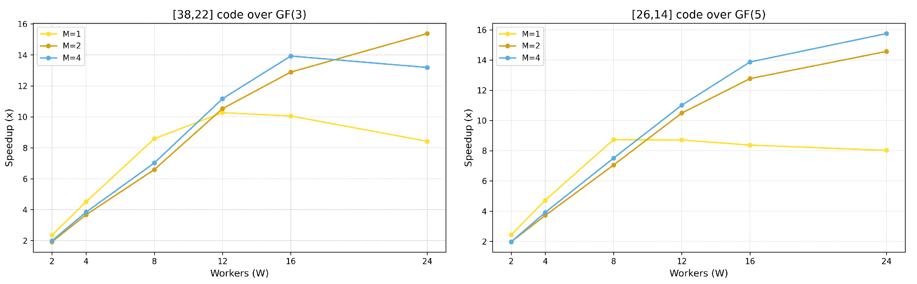
presents the computational times for an implementation with multiple master processes. Here the computations were executed on system Fujitsu Primergy RX 2540 M4 (Fujitsu Limited, Kawasaki, Japan) with 128 GB RAM, CPU 2x Intel Xeon Gold 5118 2.30 GHz 24 cores. The first four columns give the parameters of the codes for which the computations were executed, namely, q, n, k, R. The next column gives the number of master processes, followed by the columns with execution times in seconds with 1, 2, 4, 8, 16 and 24 worker processes. Computational times are given in seconds. As it can be seen from the table, with one master we observe good scalability up to 12 workers. The increase of the master processes results in slower execution in the case with one worker process. However, it can be seen that the scalability improves compared to the case with one master. This can also be seen in Figure 1, which shows the speed-up for the experimental results, given in Table 4. The speedup is calculated using the formula $T_1/T_W$, where $T_1$ is the execution time using one worker and $T_W$ is the time with W workers W = 2, 4, 8, 12, 16, 24. Figure 1 shows that when using hyperthreading (total number of processes is greater than the physical cores e.g., $W=24$), the rate with which the speed-up grows declines.

7. Conclusions

The presented algorithms in this paper give an ordering of the linear combination of columns of a matrix. This ordering allows the set of all linear combination to be enumerated and divided into close to equal to subsets. The specific characteristics of the chosen ordering also allow for efficient generation of the linear combinations. This ordering is used to parallelize an algorithm for computing the covering radius of a linear code. We developed a sequential implementation with SSE instruction and extended vector registers and a parallel implementation with a master–worker strategy. The presented sequential implementation gives good speed-up compared to the MAGMA computational algebra system and Guava package for GAP. The presented parallel implementation shows good scalability in most cases and for worker threads less than 16. We also consider an implementation with multiple master processes to improve the scalability with more worker processes. This technique further improves scalability. The experimental results show the best speedup is achieved when the total number of processes is equal to the number of physical cores. The source code of the algorithm is now available on a special page on Github: https://github.com/linearcodes-dev/CoveringRadius_MPI_implementation (accessed on 25 January 2026). In addition to the code, it also contains a description of how to compile and run it, as well as the necessary files for creating projects on different platforms with Cmake.