Towards Stable Training of Complex-Valued Physics-Informed Neural Networks: A Holomorphic Initialization Approach

Abstract

This work introduces a new initialization scheme for complex-valued layers in physics-informed neural networks that use holomorphic activation functions. The proposed method is derived empirically by estimating the activation and gradient gains specific to complex-valued tanh and sigmoid functions through Monte Carlo simulations. These estimates are then used to formulate variance-preserving initialization rules. The effectiveness of these formulas is evaluated on several second-order complex-valued ordinary differential equations derived from the Helmholtz equation, a fundamental model in wave theory and theoretical physics. Comparative experiments show that complex-valued neural solvers initialized with the proposed method outperform traditional real-valued physics-informed neural networks in terms of both accuracy and training dynamics.

1. Introduction

Differential equations are the cornerstone of mathematical models used to describe real-life physical phenomena. The analytical methods and analytical solutions for these kinds of equations are limited. As a result, solving these mathematical models reduces to using different kinds of numerical methods and computational power. One of the more recent approaches to solving ordinary and partial differential equations (ODEs/PDEs) involves the use of neural networks—a method that is theoretically explained by the foundational works of Cybenko [1], Hornik et al. [2], Poggio and Girosi [3], etc. These articles show that neural networks are universal approximators that are able to approximate any mathematical function with arbitrary accuracy.

Building on these foundational results, researchers began using neural networks to approximate solutions to differential equations by directly incorporating the equation with its initial and boundary conditions into the loss function. This idea was first explored by Lagaris et al. [4,5] and Hyuk and Kang [6], but gained significant attention just in recent years when Raissi et al. [7] introduced the term physics-informed neural networks (PINNs). The introduction of specialized libraries such as DeepXDE [8], SciANN [9], and NeuroDiffEq [10] significantly simplified the implementation of the PINN technique, in which the powerful automatic differentiation from programming is used for the differential equation inside the loss function. A comprehensive review of the applications of PINNs can be found in [11] by Karniadakis et al. or in [12], in which Mishra and Molinaro offer insights about the performance and limitations of these networks.

While numerous physical models can naturally be described using real-valued functions, there are many fundamental physical formalisms described by equations involving complex-valued functions and solutions. These complex-valued differential equations arise naturally in fields such as quantum mechanics (Schrödinger’s equation describing the evolution of quantum particles), electromagnetism (Maxwell’s equations, when formulated in the frequency domain), and wave theory (the Helmholtz equation models wave propagation in acoustics). In fluid dynamics, the complex Ginzburg–Landau equation describes systems near criticality and pattern formation in nonlinear media. The Korteweg–de Vries equation, typically studied in its real form, can also be extended to the complex domain to describe wave interactions in dispersive media. Despite their importance, complex-valued models have received less attention in the context of using neural network-based solvers. In particular, the development and analysis of complex-valued physics-informed neural networks (CVPINNs) for solving complex differential equations is a promising area of research.

There are studies in which complex-valued differential equations are solved using PINNs, such as [13,14,15,16,17]. The common approach is to split the differential equation into a coupled system of differential equations corresponding to real and imaginary parts. The internal algebra of the PINN is still a real-valued one (RVPINN) with two outputs corresponding to real and imaginary parts. The use of CVPINNs that can operate directly in the complex domain for these types of problems remains not yet fully explored. A recent study by Zhang et al. [18] compares CVPINNs and RVPINNs for solving the Gross–Pitaevskii equation, a Schrödinger-derived equation. Through their experiments, the authors solved multiple instances of this equation with CVPINN architectures and compared the results against RVPINN models. In their simulations, the CVPINNs consistently outperform RVPINNs in terms of accuracy and convergence speed. More recently, Si et al. [19] introduced a Complex Physics-Informed Neural Network (CPINN) framework that directly incorporates complex-valued unknowns into the training process. These contributions highlight an important open question: under what circumstances do CVPINNs offer a clear advantage over RVPINNs? What types of equations or setups benefit most from a fully complex-valued neural architecture? We aim to guide our research based on these questions.

In this study, we continue our previous work [20], where we employed CVPINNs to solve first-order complex-valued ODEs, demonstrating superior accuracy compared to their real-valued counterparts. Building upon that foundation, we introduce a new initialization scheme specifically designed for complex-valued layers utilizing holomorphic activation functions—particularly the holomorphic versions of tanh and sigmoid functions. This initialization method ensures stable training dynamics and is inspired by techniques commonly used in real-valued activation schemes, such as the Xavier/Glorot and He schemes [21,22,23] and more recent developments including [24], GradInit [25], and AutoInit [26]. With our improved initialization, we are able to successfully solve second-order complex-valued ODEs, such as Helmholtz-type equations arising in wave theory.

The structure of this article is as follows. In Section 2, we present foundational concepts related to initialization theory and demonstrate, through an initial experiment, how CVPINNs with poor or no initialization schemes can fail when applied to a particular case of a second-order complex-valued ODE. We derive initialization formulas for holomorphic activation functions and empirically determine the key parameters influencing these formulas. In Section 3, we apply both CVPINNs and RVPINNs to different cases of Helmholtz equation with complex coefficients. We then compare their performance in terms of accuracy against the analytical solutions. Section 4 concludes the study and discusses potential directions for future research.

2. Initialization Principles in Complex-Valued Physics-Informed Neural Networks

2.1. Initialization Theory in PINNs

In deep learning, in order to avoid the problem of vanishing or exploding gradients, the weights and biases of a neural network must be carefully initialized. We consider a fully-connected dense layer l:

$$y^{\left(l\right)}=W^{\left(l\right)}{x}^{(l-1)}+b^{\left(l\right)},$$

(1)

where $x^{(l-1)}\in {\mathbb{R}}^{n_{\mathrm{in}}}$ is the layer’s input, $W^{\left(l\right)}\in {\mathbb{R}}^{n_{\mathrm{out}}\times n_{\mathrm{in}}}$ is the weight matrix, $b^{\left(l\right)}\in {\mathbb{R}}^{n_{\mathrm{out}}}$ is the bias vector, $n_{in}$ is the number of input units for the layer (also called fan-in), and $n_{out}$ is the number of output units from the layer (also called fan-out). An initialization scheme is an algorithm for setting initial values for each layer’s weight matrix and bias vector.

A straightforward initialization would be zero initialization:

$$W^{\left(l\right)}=0, b^{\left(l\right)}=0.$$

(2)

In practice, zero initialization works just for biases (which do not affect symmetry). Initializing all weights to the same constant will make all neurons in a layer compute the same output and all gradients be identical. Using a random initialization (standard normal or uniform distribution) can also be problematic. If the variance of the weights is too large or too small, the gradients can explode or vanish through layers.

Using analytical methods, efficient initialization schemes were derived in order to preserve the variance during forward pass and gradient variance during backpropagation. Xavier initialization [21] is suitable for symmetric activation functions (such as tanh or sigmoid), while He initialization [22] is used for ReLU. The schemes use the following formulas:

$$\begin{array}{cc}\hfill {\sigma }_W^2& ={\displaystyle \frac{2}{n_{\mathrm{in}}+n_{\mathrm{out}}}} \left(\mathrm{Xavier}\right),\hfill \end{array}$$

(3)

$$\begin{array}{cc}\hfill {\sigma }_W^2& ={\displaystyle \frac{2}{n_{\mathrm{in}}}} \left(\mathrm{He}\right),\hfill \end{array}$$

(4)

where ${\sigma }_W^2$ represents the initialization variance of the weights. In the case of RVPINNs, using such an initialization scheme offers a better chance of converging to a true solution, better stability, and a faster convergence rate.

In the case of CVPINNs, we observed an initial empirical success for solving first-order ODEs, but the architectures used were simple, and luckily, they converged to a true solution in most cases even if no initialization schemes were used. We conducted an experiment in which we used a CVPINN to solve the following second-order ODE:

$${\displaystyle \frac{d^{2}f}{d{x}^2}}-i{\displaystyle \frac{df}{dx}}+2f=0,$$

(5)

where $f\left(x\right):\mathbb{R}\to \mathbb{C}$ is the unknown complex-valued function with $f\left(0\right)=1$ and $f^{\prime }\left(0\right)=2i$ as initial conditions.

We constructed different CVPINN architectures using complexReLU, tanh, and sigmoid as activation functions. The layers used are complex-valued layers containing varying numbers of randomly initialized complex neurons. complexReLU is equivalent to real ReLU applied component-wise to the real and imaginary parts, while tanh and sigmoid are holomorphic functions applied directly to the complex variable. We let the experiment run for 3000 epochs for each architecture, and we plot the loss function evolution over time for each configuration in Figure 1.

Some architectures are stable with a fast decrease in the loss function—cReLU-sigmoid, which already showed effective results in the case of first-order ODEs. Additionally, a deeper network combining six layers containing all three complex activations also shows strong convergence behavior. In contrast, some architectures behave unstable, such as multiple cReLUs or the cReLU-tanh combination. Architectures using just holomorphic activations, such as Tanh–Tanh or Sigmoid–Tanh displayed poor convergence evolutions with loss stuck around ${10}^4$. In one catastrophic case, the loss rapidly diverged and was clipped at ${10}^6$ for visualization purposes.

This initial experiment shows the necessity for specialized initialization schemes in the context of CVPINNs. Classical initialization methods such as Glorot or He were designed for real-valued neural networks and real-valued activations. Glorot or He will fail to generalize on the complex-valued holomorphic equivalents.

However, in the case of component-wise complex activation functions, such as cReLU, or applying tanh and sigmoid independently to the real and imaginary parts, we can apply modified versions of Glorot and He. A component-wise activation has the following form:

$$\varphi \left(z\right)=\varphi (x+iy)=\varphi \left(x\right)+i\varphi \left(y\right),$$

(6)

where $\varphi$ is a real-valued activation such as $\mathtt{ReLU}$, $\mathtt{tanh}$, or $\mathtt{sigmoid}$. We denote a complex weight matrix by $W=A+iB$, where $A,B\in {\mathbb{R}}^{n_{\mathrm{out}}\times n_{\mathrm{in}}}$ are initialized independently. Assuming both $A_{ij}$ and $B_{ij}$ are drawn from a zero-mean Gaussian with variance ${\sigma }^2$, the total variance of the complex weight becomes

$$Var\left[W_{ij}\right]=\mathbb{E}\left[\right|W_{ij}{|}^2]-\mathbb{E}[|W_{ij}{\left|\right]}^2=\mathbb{E}[A_{ij}^2+B_{ij}^2]=2{\sigma }^2.$$

(7)

In order to preserve variance through layers and during backpropagation for component-wise complex activations, the initialization schemes must be adjusted as follows:

$$\begin{array}{cc}\hfill {\sigma }^2& ={\displaystyle \frac{1}{n_{\mathrm{in}}+n_{\mathrm{out}}}} \left(\mathrm{Glorot}\right),\hfill \end{array}$$

(8)

$$\begin{array}{cc}\hfill {\sigma }^2& ={\displaystyle \frac{1}{n_{\mathrm{in}}}} \left(\mathrm{He}\right).\hfill \end{array}$$

(9)

Using component-wise activations, we sacrifice the mathematical structure that makes complex-valued neural networks unique. We want to use the power of holomorphic activations, so we aim to develop an analytical and computational framework for initializing complex-valued neural networks that employ truly complex holomorphic activation functions.

2.2. Generalized Initialization Strategy for Complex-Valued Networks

In order to generalize the weight initialization for complex-valued activations, we need to follow a similar mathematical approach as Glorot and He [21,22]. We will analyze how variance is transformed during forward propagation and backpropagation throughout the neural network.

We consider $x\in {\mathbb{C}}^{n_{\mathrm{in}}}$ the complex input to a fully-connected complex layer, with

$$\mathbb{E}\left[x_i\right]=0, \mathrm{Var}\left[x_i\right]={\sigma }_x^2.$$

(10)

The complex weights, $W\in {\mathbb{C}}^{n_{\mathrm{out}}\times n_{\mathrm{in}}}$, are defined such that each element is of the form $W_{ij}=A_{ij}+i{B}_{ij}$, where $A_{ij}$ and $B_{ij}$ are drawn independently from a zero-mean Gaussian with variance ${\sigma }^2$. This implies

$$\mathbb{E}\left[W_{ij}\right]=0, \mathrm{Var}\left[W_{ij}\right]=2{\sigma }^2 ={\sigma }_W^2.$$

(11)

The complex-valued preactivation is defined as

$$z_j=\sum _{i=1}^{n_{\mathrm{in}}}{W}_{ji}{x}_i,$$

(12)

on which we will apply a complex-valued activation non-element-wise activation function $\varphi \left(z\right)$.

Our goal is to find a numerical formula for the variance ${\sigma }^2$ of the complex-valued weights in order to preserve the forward variance and to ensure backward gradient stability:

$$\begin{array}{cc}\hfill \mathrm{Var}\left[\varphi \right(z\left)\right]& \approx \mathrm{Var}\left[x_i\right],\hfill \end{array}$$

(13)

$$\begin{array}{cc}\hfill \mathrm{Var}\left[{\delta }^{(l-1)}\right]& \approx \mathrm{Var}\left[{\delta }^{\left(l\right)}\right].\hfill \end{array}$$

(14)

Here, ${\delta }^{\left(l\right)}$ denotes the backpropagated error signal at layer l, defined as the derivative of the loss function $\mathcal{L}$ with respect to the preactivation $z^{\left(l\right)}$:

$${\delta }^{\left(l\right)}={\displaystyle \frac{\partial \mathcal{L}}{\partial z^{\left(l\right)}}}.$$

(15)

The variance of the preactivation will be equal to

$$\mathrm{Var}\left[z_j\right]=n_{\mathrm{in}}·{\sigma }_W^2·{\sigma }_x^2={\sigma }_z^2.$$

(16)

We use the variance formula for the activation output:

$$\mathrm{Var}\left[\varphi \left(z\right)\right]={\mathbb{E}\left[\right|\varphi \left(z\right)|}^2{]-|\mathbb{E}\left[\varphi \left(z\right)\right]|}^2.$$

(17)

For symmetric activations such as $tanh\left(z\right)$, the mean $\left|\mathbb{E}\right[\varphi \left(z\right)\left]\right|$ will vanish due to symmetry. For many other holomorphic functions, for example, sigmoid, $\left|\mathbb{E}\right[\varphi \left(z\right)\left]\right|\ne 0$, so we will retain the term for now. The last equation will approach some highly challenging complex integrals that are not solvable analytically. We can define the activation gain $\beta$, a coefficient that tells us how much of the input variance survives the activation:

$$\beta ={\displaystyle \frac{{\mathbb{E}\left[\right|\varphi \left(z\right)|}^2{]-|\mathbb{E}\left[\varphi \left(z\right)\right]|}^2}{{\sigma }_z^2}}.$$

(18)

In order to preserve forward variance, $\beta ·{\sigma }_z^2=\beta ·n_{in}·{\sigma }_W^2·{\sigma }_x^2\approx {\sigma }_x^2$, we need to have the following condition satisfied:

$$\beta ·n_{in}·{\sigma }_W^2=1.$$

(19)

During backpropagation, we propagate the gradients of the loss function through the layers as follows:

$${\delta }^{(l-1)}={\left(W^{\left(l\right)}\right)}^{\top }·\left({\delta }^{\left(l\right)}\circ {\varphi }^{\prime }\left(z^{(l-1)}\right)\right),$$

(20)

where ${\varphi }^{\prime }\left(z^{(l-1)}\right)$ is the derivative of the activation function at the previous layer, and ∘ denotes the element-wise product. Here, we made the assumption that the activation function we use is complex-differentiable and satisfies the Cauchy–Riemann equations, and we do not need to use Wirtinger calculus.

For a single unit j in layer $l-1$, we can write

$${\delta }_j^{(l-1)}={\varphi }^{\prime }\left(z_j^{(l-1)}\right)·\sum _i{W}_{ij}^{\left(l\right)}·{\delta }_i^{\left(l\right)}.$$

(21)

We need to compute the variance of the previous equation. We assume that the inputs have zero mean, and that the real and imaginary parts of the weights are initialized independently with zero mean. Under these assumptions, the backpropagated error signals ${\delta }_i^{\left(l\right)}$ also have zero mean in expectation [21,22]. Moreover, we assume independence between ${\varphi }^{\prime }\left(z_j^{(l-1)}\right)$, $W_{ij}^{\left(l\right)}$, and ${\delta }_i^{\left(l\right)}$.

With these assumptions, the last two random variables are independent and have zero mean, so the equation transforms into

$$\begin{array}{cc}\hfill \mathrm{Var}\left({\delta }_j^{(l-1)}\right)=& \left[\mathrm{Var}\left({\varphi }^{\prime }\left(z_j^{(l-1)}\right)\right)+\mathbb{E}{\left[{\varphi }^{\prime }\left(z_j^{(l-1)}\right)\right]}^2\right]·\mathrm{Var}\left(\sum _i{W}_{ij}^{\left(l\right)}{\delta }_i^{\left(l\right)}\right)\hfill \\ \hfill =& \mathbb{E}\left[{\varphi }^{\prime }{\left(z_j^{(l-1)}\right)}^2\right]·\mathrm{Var}\left(\sum _i{W}_{ij}^{\left(l\right)}{\delta }_i^{\left(l\right)}\right).\hfill \end{array}$$

(22)

We do have $n_{\mathrm{out}}$ units in layer l, so the second term of the last product becomes

$$\mathrm{Var}\left(\sum _i{W}_{ij}^{\left(l\right)}{\delta }_i^{\left(l\right)}\right)=n_{\mathrm{out}}·{\sigma }_W^2·{\sigma }_{\delta }^2.$$

(23)

We are again in the situation of solving a highly challenging complex integral that will not have a closed analytical form in most cases. We define $\gamma$ as the derivative gain, a coefficient that tells us how strong the gradient signal coming back is, relative to its input:

$$\gamma ={\displaystyle \frac{\mathbb{E}\left[\right|{\varphi }^{\prime }\left(z\right){|}^2]}{{\sigma }_z^2}}.$$

(24)

In order to preserve the backpropagation variance, $\mathrm{Var}\left({\delta }^{(l-1)}\right)\approx \mathrm{Var}\left({\delta }^{\left(l\right)}\right)={\sigma }_{\delta }^2$, we need to have the following condition satisfied:

$$\gamma ·{\sigma }_z^2·n_{out}·{\sigma }_W^2=1.$$

(25)

In order to have a stable initialization scheme, both Equations (19) and (25) need to be satisfied. Hence, we write the final formula for the total weight variance:

$${\sigma }^2={\displaystyle \frac{1}{\beta ·n_{in}+(\gamma ·{\sigma }_z)·n_{out}}}.$$

(26)

This last expression is a circular one, since ${\sigma }_z$ depends on ${\sigma }_W^2$ through ${\sigma }_z=n_{in}·{\sigma }_W^2·{\sigma }_x$, which may be solved analytically as a quadratic or approximated numerically. Alternatively, one can introduce empirical simplifications based on simulation results. For the purposes of this analysis, the expression (26) is taken as the final form.

2.3. Empirical Estimation of Gain Parameters

The activation gain $\beta$ and its derivative gain $\gamma$ must be estimated in order to have the final form of the complex initialization scheme. As we stated earlier, computing the integrals involved for activation functions such as $tanh\left(z\right)$ or $\mathtt{sigmoid}\left(z\right)$ is not an easy analytical task. In order to overcome this, we will estimate the gains numerically by sampling complex Gaussian inputs and using Monte Carlo simulations to approximate and plot the gains, along with the product $\gamma ·{\sigma }_z$, which appears in the denominator of (26). Figure 2 shows the estimated values of $\beta$, $\gamma$, and $\gamma ·{\sigma }_z$ as a function of the input variance ${\sigma }_z^2$ for both the $tanh\left(z\right)$ and $\mathtt{sigmoid}\left(z\right)$ activation functions.

Based on the empirical plots, we can now extract approximate values of the gain parameters in order to rewrite our formula. For the $tanh\left(z\right)$ activation, $\beta$ is noisy with overall values in the range $[1,5]$, but we can stabilize $\beta \approx 3$ especially for input variances in the interval $[0,3]$. Although the gradient gain $\gamma$ decreases rapidly as the variance increases, we observe that the product $\gamma ·{\sigma }_z$ remains relatively stable across the same range. This allows us to approximate $\gamma ·{\sigma }_z\approx 1.8$. For the $\mathtt{sigmoid}\left(z\right)$ activation, the gains are smaller, with $\beta \approx 0.6$ and $\gamma ·{\sigma }_z\approx 0.3$. Substituting these empirically found constants into the general formula (26) leads to the following initialization schemes:

$$\begin{array}{cc}\hfill {\sigma }^2& ={\displaystyle \frac{1}{3·n_{\mathrm{in}}+1.8·n_{\mathrm{out}}}} (\mathrm{complex} tanh),\hfill \end{array}$$

(27)

$$\begin{array}{cc}\hfill {\sigma }^2& ={\displaystyle \frac{1}{0.6·n_{\mathrm{in}}+0.3·n_{\mathrm{out}}}} (\mathrm{complex} \mathrm{sigmoid}).\hfill \end{array}$$

(28)

We can use these empirical formulas in a series of experiments in which we construct different CVPINN architectures using the holomorphic tanh and sigmoid as activations. We use three CVPINNs, one using just complex-valued layers with tanh activations, another using only sigmoid as activations, and one combining both. Each CVPINN is trained under three initialization strategies: a standard random initialization, the real-valued Glorot scheme applied to real and imaginary parts, and our empirical activation scheme formulas. All CVPINN cases were trained for 1000 epochs, and the results are visualized in Figure 3.

We observe from the plots that CVPINNs initialized with our empirical activation-dependent schemes achieve the best performance for all three architectures. They reach loss values up to two orders of magnitude lower than those initialized with other methods.

3. Experimental Validation on Differential Equation Benchmarks

In order to validate our proposed initialization strategy, we designed a series of experiments in which we train in parallel a CVPINN model and an RVPINN model on the same complex physics-inspired ODE. The results obtained by both networks will later be compared with the true analytical solutions. The equations are chosen to reflect different aspects of wave-like behavior in complex domains, with all of them being modified versions of the Helmholtz equation:

$${\nabla }^{2}f=-k^{2}f,$$

(29)

where ${\nabla }^2$ is the Laplacian operator, while $f\left(0\right)=f_0$ and $f^{\prime }\left(0\right)=f_0^{\prime }$ are the initial conditions. All our experiments were designed as one-dimensional equations defined over the domain $x\in [0,5]$, with 5000 collocation points and identical fixed initial conditions for CVPINN and RVPINN architectures. The CVPINN is constructed using the holomorphic activations $tanh\left(z\right)$ and $\mathtt{sigmoid}\left(z\right)$, arranged in an alternating sequence across fully connected complex-valued layers. This network uses our activation-aware initialization scheme to stabilize learning.

In contrast, the RVPINN is designed as a double-output neural network that approximates the real and imaginary parts of the solution as a coupled scalar function. To ensure a fair comparison in terms of parameter count, each RVPINN layer contains twice the number of neurons as its CVPINN counterpart. Real-valued Xavier initialization is applied to the weights of RVPINNs.

In the case of CVPINNs, the solution is modeled as a complex-valued function $f\left(x\right):\mathbb{R}\to \mathbb{C}$. Automatic differentiation is used to compute the required first and second derivatives with respect to the real input. The total loss for the CVPINN is defined as

$${\mathcal{L}}_{\mathrm{CV}}={\lambda }_{\mathrm{ODE}}·{\mathcal{L}}_{\mathrm{res}}+{\lambda }_{\mathrm{IC}}·\left(\parallel f\left(0\right)-f_0{\parallel }^2+{\parallel f^{\prime }\left(0\right)-f_0^{\prime }\parallel }^2\right),$$

(30)

where ${\mathcal{L}}_{\mathrm{res}}$ is the mean squared error of the PDE residuals, while the weights ${\lambda }_{\mathrm{ODE}}$ and ${\lambda }_{\mathrm{IC}}$ balance the contributions of the physical constraint and the initial data.

For RVPINNs, the solution $f\left(x\right)$ is decomposed into the real and imaginary parts: $f\left(x\right)=u\left(x\right)+iv\left(x\right)$, where $u\left(x\right),v\left(x\right)\in \mathbb{R}$. The original complex differential equation is reformulated as a coupled system of two real-valued differential equations involving both u and v, as well as their respective derivatives. This transformation results in a system of the form

$$\begin{array}{cc}\hfill {\mathcal{N}}_u[u,v]& =0,\hfill \end{array}$$

(31)

$$\begin{array}{cc}\hfill {\mathcal{N}}_v[u,v]& =0.\hfill \end{array}$$

(32)

The total loss function for the RVPINN is defined as

$${\mathcal{L}}_{\mathrm{RV}}={\lambda }_{\mathrm{ODE}}·\left(\parallel {\mathcal{N}}_u{\parallel }^2+{\parallel {\mathcal{N}}_v\parallel }^2\right)+{\lambda }_{\mathrm{IC}}·{\mathcal{L}}_{\mathrm{IC}},$$

(33)

where

$${\mathcal{L}}_{\mathrm{IC}}=\parallel u\left(0\right)-\mathrm{Re}\left(f_0\right){\parallel }^2+\parallel v\left(0\right)-\mathrm{Im}\left(f_0\right){\parallel }^2+\parallel u^{\prime }\left(0\right)-\mathrm{Re}\left(f_0^{\prime }\right){\parallel }^2+{\parallel v^{\prime }\left(0\right)-\mathrm{Im}\left(f_0^{\prime }\right)\parallel }^2.$$

(34)

This formulation ensures that both models are trained under consistent physical and boundary constraints, facilitating a direct comparison between the expressivity and training stability of CVPINNs and RVPINNs. All derivative terms are computed via automatic differentiation. Each PINN is trained for 5000 epochs using the Adam optimizer with a learning rate scheduler that decays the learning rate 70% every 500 epochs.

3.1. Undamped Complex Helmholtz Equation

The first benchmark considers the canonical Helmholtz equation with a complex wavenumber, with its value fixed and used in later experiments:

$${\displaystyle \frac{d^{2}f}{d{x}^2}}+k^{2}f\left(x\right)=0, k=2\pi +i.$$

(35)

In this initial experiment, we set the initial conditions to

$$f\left(0\right)=1, f^{\prime }\left(0\right)=ik=-1+2\pi i.$$

(36)

This equation admits the following exact solution:

$$f\left(x\right)=e^{ikx}.$$

(37)

This case models complex wave propagation in homogeneous media. Simulation results are shown in Figure 4.

The CVPINN closely follows the analytical solution in both the real and imaginary components, accurately capturing the oscillatory behavior. In contrast, the RVPINN fails to learn the wave dynamics, quickly flattening out and diverging from the true solution. The loss curve shows that the CVPINN is converging smoothly, while RVPINN stagnates at a high loss value.

3.2. Damped Complex Helmholtz Equation

To evaluate performance on more complex systems, we consider the damped Helmholtz equation

$${\displaystyle \frac{d^{2}f}{d{x}^2}}+2\alpha {\displaystyle \frac{df}{dx}}+k^{2}f\left(x\right)=0, \alpha =0.5,$$

(38)

with the following initial conditions:

$$f\left(0\right)=1, f^{\prime }\left(0\right)=(-\alpha +ik)f\left(0\right).$$

(39)

The analytical solution becomes

$$f\left(x\right)=e^{-\alpha x}·e^{ikx}.$$

(40)

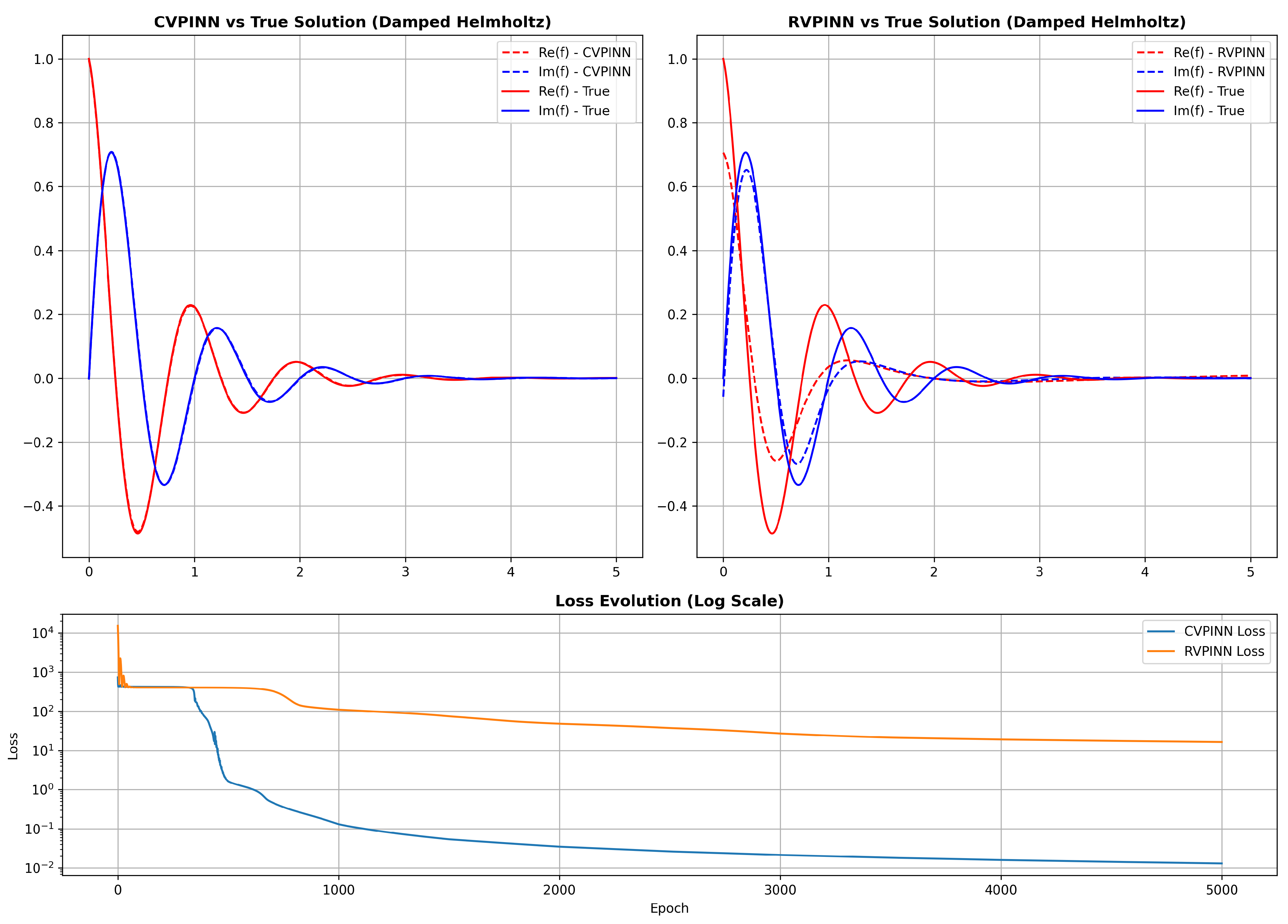
This equation reflects dissipative effects common in electromagnetism and acoustics. Simulation results are shown in Figure 5.

The CVPINN successfully models the decaying wave pattern, preserving both phase and amplitude accuracy. The RVPINN captures the general decay trend but struggles with phase alignment and underestimates amplitude. The loss evolution again highlights the superior convergence for CVPINN compared to the slowly declining and plateaued RVPINN.

3.3. Forced Complex Helmholtz Equation

In the third benchmark, we aim to solve a more complex ODE in which we introduced a nonhomogeneous term but that still possesses an analytical solution. We introduce the term $2ik{e}^{ikx}$ as a forcing term to the Helmholtz equation:

$${\displaystyle \frac{d^{2}f}{d{x}^2}}+k^{2}f\left(x\right)=2ik{e}^{ikx}.$$

(41)

We set the initial conditions to

$$f\left(0\right)=0, f^{\prime }\left(0\right)=1.$$

(42)

The previous equation admits the following analytical solution:

$$f\left(x\right)=x{e}^{ikx}.$$

(43)

This equation models a wave field driven by a harmonic source and is commonly encountered in problems involving acoustic or electromagnetic scattering. Simulation results are presented in Figure 6.

The CVPINN captures both the linear amplitude growth and the oscillatory structure of the exact solution with high fidelity. RVPINN predictions diverge early and fail to represent the increasing wave profile. The loss curves confirm that CVPINN achieves a low training error, while RVPINN remains trapped at high loss levels.

3.4. Two-Dimensional Helmholtz Equation Simulation

To further demonstrate that the proposed initialization strategy is not limited to one-dimensional problems, we considered a two-dimensional Helmholtz equation with a forcing term on the unit square domain $\mathsf{\Omega }=[0,1]\times [0,1]$.

The governing PDE is

$${\nabla }^{2}u(x,y)+k^{2}u(x,y)=f(x,y), (x,y)\in \mathsf{\Omega },$$

(44)

with complex wave number $k=2.0+0.5i$. Dirichlet boundary conditions were prescribed on all four edges, matching the analytical solution

$$u(x,y)=sin\left(\pi x\right) sin\left(\pi y\right) e^{ikx}.$$

(45)

This choice of $u(x,y)$ allows us to construct both the forcing term

$$f(x,y)={\nabla }^{2}u(x,y)+k^{2}u(x,y)$$

(46)

and the boundary conditions exactly. Moreover, it provides a closed-form reference against which $L_2$ errors can be evaluated.

We compared a CVPINN and an RVPINN. The CVPINN directly maps $(x,y)\in {\mathbb{R}}^2$ to complex outputs using holomorphic activations, with an architecture similar to that used in the one-dimensional experiments, alternating tanh and sigmoid activations. The RVPINN treats the real and imaginary parts separately, employing a comparable depth and the number of layers, with two outputs corresponding to $\Re \left(u\right)$ and $\Im \left(u\right)$.

The training loss consists of two contributions:

• The PDE residual inside the domain. For the CVPINN, this is

  $${\mathcal{L}}_{\mathrm{PDE}}={\displaystyle \frac{1}{N_{\mathsf{\Omega }}}}\sum _{(x,y)\in \mathsf{\Omega }}|{\nabla }^2{u}_{\theta }(x,y)+k^2{u}_{\theta }(x,y)-f(x,y){|}^2.$$

  (47)
  For the RVPINN, the complex PDE is split into two coupled real equations for the real and imaginary components.
• The boundary condition residual is

  $${\mathcal{L}}_{\mathrm{BC}}={\displaystyle \frac{1}{N_{\partial \mathsf{\Omega }}}}\sum _{(x,y)\in \partial \mathsf{\Omega }}|u_{\theta }(x,y)-u(x,y){|}^2.$$

  (48)

The total loss is defined as

$$\mathcal{L}={\mathcal{L}}_{\mathrm{PDE}}+\lambda {\mathcal{L}}_{\mathrm{BC}}, \lambda =10,$$

(49)

providing stronger enforcement for the boundary conditions.

Both networks were trained with $N_{\mathsf{\Omega }}=2500$ interior collocation points and $N_{\partial \mathsf{\Omega }}=400$ boundary points, using the Adam optimizer with a learning rate ${10}^{-3}$ and a step decay schedule. Training ran for 5000 epochs.

Figure 7 shows the real and imaginary parts of the learned solution for both the CVPINN and RVPINN, together with the true solution. The results indicate that both models are able to capture the main patterns of the solution with good accuracy. However, the CVPINN achieves a slightly better match, reflected in a lower $L_2$ error norm overall. Here, the $L_2$ error is computed as

$$\parallel u_{\theta }{-u\parallel }_2={\left({\displaystyle \frac{1}{N}}\sum _{j=1}^N|u_{\theta }(x_j,y_j)-u(x_j,y_j){|}^2\right)}^{\frac{1}{2}},$$

(50)

where $u_{\theta }$ is the network prediction, u is the analytical solution, and ${\left\{(x_j,y_j)\right\}}_{j=1}^N$ are evaluation points in the domain. This quantitative comparison shows that, while both PINN formulations work well in two dimensions, the complex-valued formulation provides an improvement in accuracy.

4. Conclusions

In this study, we introduced initialization scheme formulas for CVPINNs with holomorphic activation functions, such as tanh and sigmoid, addressing a critical bottleneck in the training dynamics and stability of models needed for solving complex-valued ODEs. CVPINNs introduce challenges in terms of finding a stable and correct solution due to their complex nature, working directly in the complex domain, that makes the well-known Glorot or He initializations insufficient. In order to overcome this, we derived a variance-preserving initialization framework inspired by classical approaches but adapted to the complex domain.

Using Monte Carlo simulations, we empirically estimated the activation and gradient gains associated with complex-valued tanh and sigmoid activations. We formulated final initialization formulas that we experimentally validated on a particular case of a complex-valued ODE. Our initialization strategy was evaluated on a series of benchmark problems derived from the complex-valued Helmholtz equation, covering scenarios with known analytical solutions: undamped, damped, forced wave, and a two-dimensional scenario.

The numerical results consistently show that CVPINNs initialized using our scheme significantly outperform RVPINNs that split the ODE into a system of coupled ODEs corresponding to real and imaginary parts. CVPINNs were more effective at capturing amplitude dynamics, phase oscillations, and non-trivial growth patterns—particularly in the forced Helmholtz case, where RVPINNs failed to generalize. In all benchmarks, CVPINNs also showed smoother loss curves and faster convergence. These findings confirm that operating directly in the complex domain, with initializations tailored for holomorphic processing, provides both theoretical and practical advantages.

In addition to accuracy improvements, our results also reinforce the initial observation we had in [20] that operating in the complex domain provides a richer mathematical framework for solving ODEs/PDEs. Holomorphic functions may improve the learning capacity of neural networks, especially when properly initialized. Complex-valued algebra also increases computational workload, and training such networks requires more memory and processing time. Despite the additional computational cost, our results show that CVPINNs can be a viable and effective tool—especially when ample computing resources are available and when systems are intrinsically complex-inherent models.

Building on these findings, we state some potential future research directions. First is the extension of our initialization scheme to more advanced network architectures, such as convolutional or residual CVPINNs. Second, the development and testing of deeper or wider CVPINN architectures on more challenging complex-valued ODEs and PDEs—particularly in higher dimensions—would provide a better overview of this method. Third, there is strong motivation to investigate the application of CVPINNs to spectral or eigenvalue problems in the complex domain, where computational methods are limited. Progress in this area could significantly advance data-driven modeling and theoretical physics, especially in quantum mechanics or complex wave propagation.

References

1. Cybenko, G. Approximation by superpositions of a sigmoidal function. Math. Control. Signals Syst. 1989, 2, 303–314. [Google Scholar] [CrossRef]
2. Hornik, K.; Stinchcombe, M.; White, H. Multilayer feedforward networks are universal approximators. Neural Netw. 1989, 2, 359–366. [Google Scholar] [CrossRef]
3. Poggio, T.; Girosi, F. Networks for approximation and learning. Proc. IEEE 1990, 78, 1481–1497. [Google Scholar] [CrossRef]
4. Lagaris, I.; Likas, A.; Fotiadis, D. Artificial neural networks for solving ordinary and partial differential equations. IEEE Trans. Neural Netw. 1998, 9, 987–1000. [Google Scholar] [CrossRef]
5. Lagaris, I.; Likas, A.; Papageorgiou, D. Neural-network methods for boundary value problems with irregular boundaries. IEEE Trans. Neural Netw. 2000, 11, 1041–1049. [Google Scholar] [CrossRef]
6. Lee, H.; Kang, I.S. Neural algorithm for solving differential equations. J. Comput. Phys. 1990, 91, 110–131. [Google Scholar] [CrossRef]
7. Raissi, M.; Perdikaris, P.; Karniadakis, G.E. Physics-informed neural networks: A deep learning framework for solving forward and inverse problems involving nonlinear partial differential equations. J. Comput. Phys. 2017, 378, 686–707. [Google Scholar] [CrossRef]
8. Lu, L.; Meng, X.; Mao, Z.; Karniadakis, G.E. DeepXDE: A deep learning library for solving differential equations. SIAM Rev. 2021, 63, 208–228. [Google Scholar] [CrossRef]
9. Haghighat, E.; Juanes, R. SciANN: A Keras/TensorFlow wrapper for scientific computations and physics-informed deep learning using artificial neural networks. Comput. Methods Appl. Mech. Eng. 2021, 373, 113552. [Google Scholar] [CrossRef]
10. Chen, F.; Sondak, D.; Protopapas, P.; Mattheakis, M.; Liu, S.; Agarwal, D.; Di Giovanni, M. NeuroDiffEq: A Python package for solving differential equations with neural networks. J. Open Source Softw. 2020, 5, 1931. [Google Scholar] [CrossRef]
11. Karniadakis, G.E.; Raissi, M.; Perdikaris, P. Physics-informed machine learning. Nat. Rev. Phys. 2021, 3, 422–440. [Google Scholar] [CrossRef]
12. Mishra, S.; Molinaro, R. Estimates on the generalization error of physics-informed neural networks for approximating PDEs. IMA J. Numer. Anal. 2022, 42, 2277–2305. [Google Scholar] [CrossRef]
13. Pu, J.C.; Li, J.; Chen, Y. Soliton, breather, and rogue wave solutions for solving the nonlinear Schrödinger equation using a deep learning method with physical constraints. Chin. Phys. B 2021, 30, 060202. [Google Scholar] [CrossRef]
14. Pu, J.; Chen, Y. Complex dynamics on the one-dimensional quantum droplets via time piecewise PINNs. Phys. D Nonlinear Phenom. 2023, 454, 133851. [Google Scholar] [CrossRef]
15. Wang, S.; Li, B.; Chen, Y.; Perdikaris, P. PirateNets: Physics-informed Deep Learning with Residual Adaptive Networks. J. Mach. Learn. Res. 2024, 25, 1–51. [Google Scholar]
16. Kashefi, A.; Mukerji, T. Physics-informed PointNet: A deep learning solver for steady-state incompressible flows and thermal fields on multiple sets of irregular geometries. J. Comput. Phys. 2022, 468, 111510. [Google Scholar] [CrossRef]
17. Mahmoudabadbozchelou, M.; Karniadakis, G.E.; Jamali, S. nn-PINNs: Non-Newtonian Physics-Informed Neural Network for complex fluids modeling. Soft Matter 2021, 18, 172–185. [Google Scholar] [CrossRef]
18. Zhang, L.; Mengge, D.; Bai, X.; Chen, Y.; Zhang, D. Complex-valued physics-informed machine learning for efficient solving of quintic nonlinear Schrödinger equations. Phys. Rev. Res. 2025, 7, 013164. [Google Scholar] [CrossRef]
19. Si, C.; Yan, M.; Li, X.; Xia, Z. Complex Physics-Informed Neural Network. arXiv 2025, arXiv:2502.04917. [Google Scholar] [CrossRef]
20. Mohuț, A.I.; Popa, C.A. When Should We Use Complex-Valued PINNs? Case Study on First-Order ODEs. 2025; Manuscript submitted for publication. [Google Scholar]
21. Glorot, X.; Bengio, Y. Understanding the difficulty of training deep feedforward neural networks. In Proceedings of the Thirteenth International Conference on Artificial Intelligence and Statistics; Teh, Y.W., Titterington, M., Eds.; Chia Laguna Resort: Sardinia, Italy, 2010; Volume 9, pp. 249–256. [Google Scholar]
22. He, K.; Zhang, X.; Ren, S.; Sun, J. Delving Deep into Rectifiers: Surpassing Human-Level Performance on ImageNet Classification. In Proceedings of the 2015 IEEE International Conference on Computer Vision (ICCV), Santiago, Chile, 7–13 December 2015; pp. 1026–1034. [Google Scholar] [CrossRef]
23. Lecun, Y.; Bottou, L.; Orr, G.; Müller, K.-R. Efficient BackProp. 2000. Available online: https://cseweb.ucsd.edu/classes/wi08/cse253/Handouts/lecun-98b.pdf (accessed on 20 August 2025).
24. Maciej, S.; Alessandro, T.; Martin, T. Revisiting Initialization of Neural Networks. arXiv 2020, arXiv:2004.09506. [Google Scholar] [CrossRef]
25. Zhu, C.; Ni, R.; Xu, Z.; Kong, K.; Huang, w.R.; Goldstein, T. GradInit: Learning to Initialize Neural Networks for Stable and Efficient Training. Proc. Adv. Neural Inf. Process. Syst. 2021, 34, 16410–16422. [Google Scholar]
26. Garrett, B.; Risto, M. AutoInit: Analytic Signal-Preserving Weight Initialization for Neural Networks. arXiv 2022, arXiv:2109.08958. [Google Scholar]
Figure 1. Training loss evolution (log scale) for CVPINNs with different activation architectures. Each model is trained for 3000 epochs to solve a second-order ODE: f ( x ) i f ( x ) + 2 f = 0 with f ( 0 ) = 1 , f ( 0 ) = 2 i as initial conditions. The function domain is x [ 0 , 10 ] with 1000 collocation points. All layers are randomly initialized. Training is performed using the Adam optimizer with a learning rate scheduler.
Mathematics 14 00435 g001
Figure 2. Empirical estimation of gain parameters for tanh and sigmoid holomorphic activation functions.
Mathematics 14 00435 g002
Figure 3. Training loss comparison of CVPINNs using different initialization schemes for three architectures. Each architecture is tested with standard random initialization, real-valued Glorot initialization, and our proposed empirical activation formulas.
Mathematics 14 00435 g003
Figure 4. Comparison of CVPINN and RVPINN predictions with the analytical solution for the undamped complex Helmholtz equation.
Mathematics 14 00435 g004
Figure 5. Comparison of CVPINN and RVPINN predictions with the analytical solution for the damped complex Helmholtz equation.
Mathematics 14 00435 g005
Figure 6. Comparison of CVPINN and RVPINN predictions with the analytical solution for the forced complex Helmholtz equation.
Mathematics 14 00435 g006
Figure 7. Two-dimensional Helmholtz equation: comparison between true solution, CVPINN, and RVPINN. Top: real parts. Middle: imaginary parts. Bottom: training loss curves and L 2 error comparison.
Mathematics 14 00435 g007
Disclaimer/Publisher’s Note: The statements, opinions and data contained in all publications are solely those of the individual author(s) and contributor(s) and not of MDPI and/or the editor(s). MDPI and/or the editor(s) disclaim responsibility for any injury to people or property resulting from any ideas, methods, instructions or products referred to in the content.