Abstract
This study addresses the problem of estimating parameters in a two-threshold Ornstein–Uhlenbeck diffusion process, a model suitable for describing systems that exhibit changes in dynamics when crossing specific boundaries. Such behavior is often observed in real economic and physical processes. The main objective is to develop and evaluate a method for accurately identifying key parameters, including the threshold levels, drift changes, and diffusion coefficient, within this stochastic framework. The paper proposes an iterative algorithm based on approximate maximum likelihood estimation, which recalculates parameter values step by step until convergence is achieved. This procedure simultaneously estimates both the threshold positions and the associated process parameters, allowing it to adapt effectively to structural changes in the data. Unlike previously studied single-threshold systems, two-threshold models are more natural and offer improved applicability. The method is implemented through custom programming and tested using synthetically generated data to assess its precision and reliability. The novelty of this study lies in extending the approximate maximum likelihood framework to a two-threshold Ornstein–Uhlenbeck process and in developing an iterative estimation procedure capable of jointly recovering both threshold locations and regime-specific parameters with proven convergence properties. Results show that the algorithm successfully captures changes in the process dynamics and provides consistent parameter estimates across different scenarios. The proposed approach offers a practical tool for analyzing systems influenced by shifting regimes and contributes to a better understanding of dynamic processes in various applied fields.
Keywords:
approximate maximum likelihood method; two-threshold diffusion process; stochastic differential equation MSC:
37M25; 60H10
1. Introduction
The threshold effect refers to a phenomenon in which changes in an outcome remain minimal or nonexistent while a variable changes up to a certain point. Once this threshold is exceeded, the effect becomes abrupt or highly pronounced. Numerous studies have focused on developing and analyzing stochastic models that incorporate threshold effects, for example [1,2]. Modeling systems with multiple threshold effects also represents an important practical challenge. For instance, in finance, small increases in income can trigger a sharp change in the effective tax rate once a threshold is crossed [3]. In clinical pharmacology, the therapeutic efficacy of a drug exhibits a concentration-dependent profile, in which sub-therapeutic or supra-therapeutic blood concentrations can result in diminished effectiveness or adverse effects, respectively [4]. Here, there are both minimum and maximum safe thresholds. Unlike single-threshold models, two-threshold models more naturally reflect such real-world processes and allow for greater flexibility in capturing regime dynamics [5,6].
Similarly, the Ornstein–Uhlenbeck process considered in this article is used to describe phenomena that tend to fluctuate around an equilibrium state under the influence of random noise [7]. For instance, it is commonly applied to the modeling of interest rates, asset prices, and other financial variables [8]. Threshold diffusion processes of this type enable the analysis of distinct dynamic regimes while accounting for the current state of the system [9,10,11].
Gaussian-type threshold diffusion models that incorporate location shifts have been investigated in [8,12,13,14]. Parameter estimation techniques for single-threshold models were examined in [9,12]. A quasi-probabilistic method for estimating shift parameters in two-regime threshold diffusion processes was proposed in [15]. In [13], an initial testing procedure based on an approximate maximum likelihood framework was developed to assess linearity of the diffusion process and the presence of threshold effects in both drift and diffusion components. Convergence properties, which constitute a key aspect of the asymptotic behavior of the approximate maximum likelihood estimator, were analyzed in [16,17,18].
Unlike Bayesian methods, which rely on simulating parameter distributions through random sampling and require prior assumptions about their values [19], the AMLE approach provides direct parameter estimation based on the likelihood function without using such prior hypotheses, which significantly simplifies computations.
Compared to the Expectation–Maximization (EM) algorithm [20], which iteratively maximizes conditional expectations and may exhibit slow convergence in complex or flat regions of the parameter space, the proposed iterative AMLE procedure employs explicit numerical updates with a convergence check based on the spectral radius condition 1.
This study investigates a two-threshold, three-mode Ornstein–Uhlenbeck diffusion process. The purpose of the study is to develop an approximate log-likelihood function for a process of this type, as well as to estimate the parameters of each of the modes and determine the threshold values, and to verify the proposed methodological approach using software code.
We employed a comprehensive set of methods to achieve this goal. The process was discretized by the Euler scheme, and a likelihood function was formed. The set of parameters for each mode is calculated by solving a system of equations with coefficients that take into account the variability of the data. The threshold values are calculated using an iterative algorithm in which, at each step the mode boundaries are checked for convergence.
The remainder of the paper is structured as follows: Section 2 outlines the mathematical background and discusses existing approaches to modeling systems with threshold behavior; Section 3 introduces the proposed iterative algorithm for estimating model parameters and threshold values; Section 4 details the iterative estimation procedure and explains the convergence criteria; Section 5 presents the numerical implementation, describes the simulation setup, and reports the main results; and Section 6 concludes the paper with a summary of findings and potential directions for future research.
2. Mathematical Background and Approaches to Research
The Ornstein–Uhlenbeck process [21], which has a number of properties (stationarity, Gaussianity, Markov property), is defined from the stochastic differential Equation (1):
where is the state variable at time ; is mean-reversion rate, indicating how quickly the process tends to return to the long-term mean ; is the diffusion coefficient, representing the intensity of the random fluctuations; is a Wiener process (or standard Brownian motion), , .
Equation (1) has an analytical solution at [9]:
Unlike the single-threshold systems commonly examined in the literature [10], the present study advances the methodological framework by introducing two distinct threshold values into the stochastic process. This extension facilitates the representation of systems governed by three operational regimes, thereby improving the model’s ability to capture more complex and realistic dynamics. Two-threshold models are especially useful in applications where structural shifts occur in a non-symmetric or multi-phase manner, such as in economics, climatology, and biological systems [5,22]. By incorporating an intermediate state between two extreme regimes, this approach offers a more natural and flexible characterization of real-world processes in which transitions across multiple dynamic states frequently arise.
Accordingly, the stochastic process with two modes and two thresholds can be mathematically formulated as follows in Equation (2):
where , ,—determine the linear shift in the -th mode (), and —the diffusion coefficient in this mode. The process is divided by thresholds and into three modes and each mode has different shift and diffusion coefficients. The behavior of the Ornstein–Uhlenbeck process with two thresholds changes depending on which of the three modes is in.
In applied problems, the analysis of a stochastic process is carried out at discrete points in time, so we will consider a discretized version of the process. Let be a set of data of the process , which were obtained at times {, where , is the time step between the obtained values.
To discretize stochastic differential equations, we will use the Euler scheme (3):
where increment of the Wiener process, and the time step of discretization . If the values of and , are available, then from expression (3) we can obtain the function of doubled negative log-likelihood .
As a result, for each value of , given the previous value of , the approximation provides a normal distribution of the increment
for some constant , which does not affect the estimation by the maximum likelihood method.
The system of equations for estimating the model parameters will include the following model parameters: , for thresholds and .
Differentiating the equation by the shift parameters:
at
:
at :
at :
Differentiation of the equation with respect to the diffusion parameters , , :
By equating the results of differentiation by parameters to zero, we obtain a system of equations for the parameters in matrix form:
Thus, the system of equations for parameter estimation consists of a separate selection of parameters for each mode using the given model. The results depend on the values of the thresholds and , which divide the trajectory into subsets. These equations are used as the basis for an iterative algorithm for parameter and threshold estimation.
3. Iterative Algorithm for Estimating Parameters and Thresholds
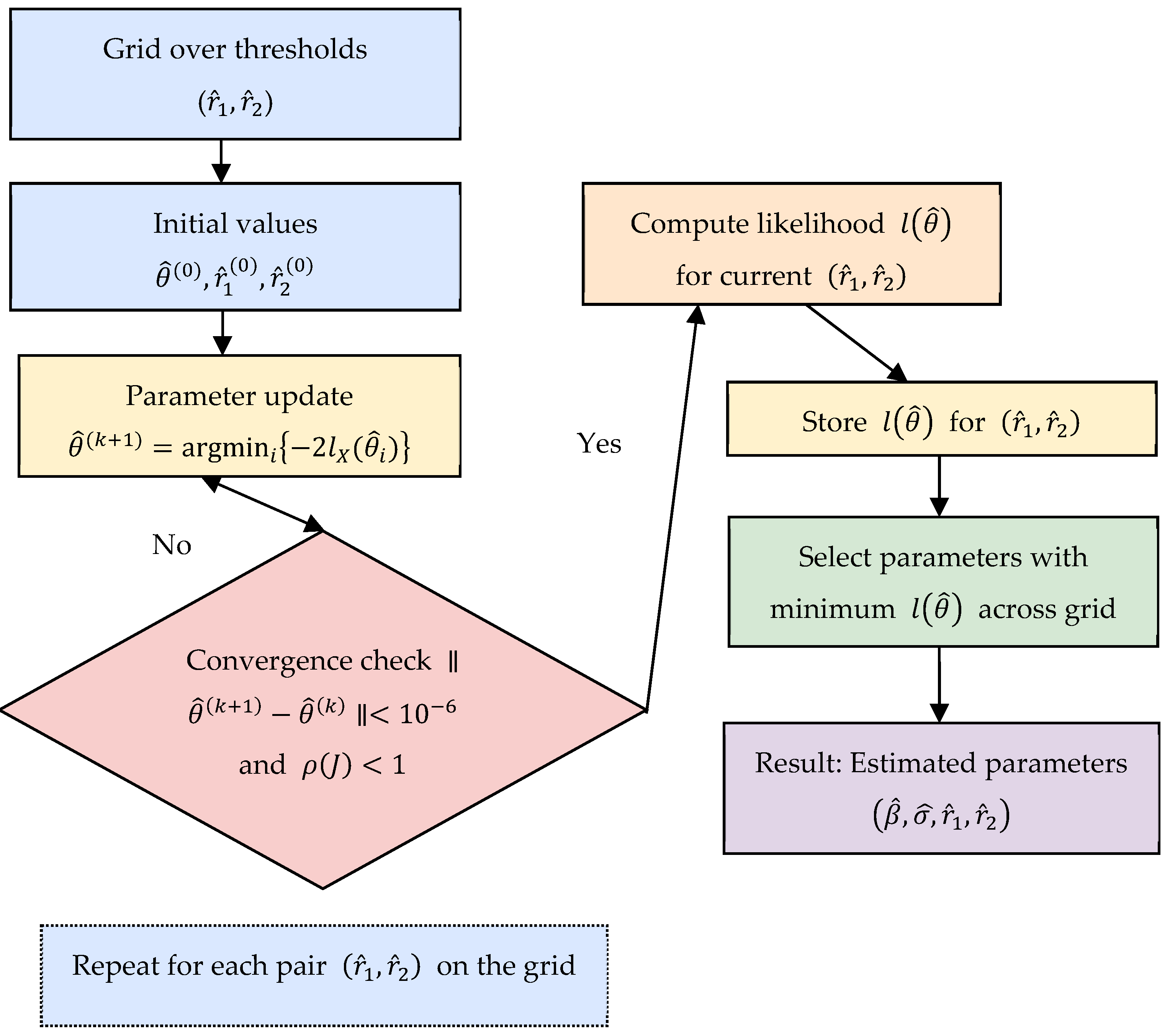
The calculation of the parameters and the thresholds , in the three-mode two-threshold Ornstein–Uhlenbeck process can be accomplished using the improved iterative algorithm (Figure 1) described in [8], as outlined below. an estimated value of the parameters. The estimation procedure proceeds iteratively until convergence is achieved.

Figure 1.
Block diagram of the Iterative Algorithm for Estimating Parameters and Thresholds.
Step 1. Initialization.
Time series , for which the ordinal statistics are calculated, where
Step 2. Iterative Estimation.
2.1. It is necessary to fix the threshold vector for , and initialize the variance estimates λ is the index limit (the number of tested parameter combinations).
2.2. For each iteration , we update the parameter vector
recursively using the update equations (see Equation (5)). In each equation, the previous iteration’s values by by , i = 1, 2, 3; j = 0, 1.
2.3. Repeat Step 2.2 until the estimated value of the parameter vector is convergent. In our implementation, convergence is assessed using a tolerance of and the spectral analysis of the Jacobian matrix (see Section 4 for details).
Let the convergent estimate be of the form
Step 3. Model Selection.
For each , compute the negative log-likelihood value . Then select the index that gives the highest likelihood and define the approximate maximum likelihood estimate of the full parameter set as .
4. Iterative Parameter Estimation Procedure
The parameter estimation for the two-threshold Ornstein–Uhlenbeck (OU) process with three dynamic regimes involves solving a complex optimization problem due to the presence of non-linearities and regime-dependent structural breaks. The model assumes that the observed stochastic process transitions between three distinct modes, each governed by its own drift and diffusion coefficients, with the transitions determined by two unknown thresholds and . The parameter vector to be estimated is defined as
where are the drift parameters and are the regime-specific diffusion variances for i = 1, 2, 3 and j = 0, 1. The model captures the piecewise linear behavior of the system dynamics over the intervals . The initial thresholds are generated over a uniform grid within the range of observed data , excluding 5% at both ends to avoid empty regimes. For each pair , the initial variance parameters are set to half of the empirical variance of observations within the corresponding region. The regression coefficients are then estimated analytically in the first iteration using the normal equations.
This data-driven initialization provides stable starting values and ensures convergence without requiring arbitrary parameter assumptions.
To estimate these parameters, an iterative numerical procedure is employed, leveraging the structure of the Approximate Maximum Likelihood Estimation (AMLE). At the core of the algorithm lies a fixed-point iteration scheme, where the current estimate of the parameter vector at iteration is updated via a transformation function , such that
The mapping is defined implicitly by the likelihood function, and incorporates regime segmentation, parameter re-estimation, and variance update steps. Specifically, each iteration proceeds as follows:
- Segmentation. The dataset is partitioned into three subsets based on current estimates of the thresholds and . This segmentation defines the data points corresponding to each regime.
- Parameter Update. Within each regime, drift parameters are estimated via linear regression using least-squares or generalized method of moments, and diffusion parameters are updated based on the empirical variance of the residuals. These estimators exploit the local linearity of the OU process and assume conditional independence of the noise terms across time steps.
- Threshold Optimization. Updated thresholds may be obtained via grid search or gradient-based optimization techniques aimed at maximizing the approximate likelihood. Alternatively, a profile likelihood approach may be employed where the likelihood is maximized over thresholds for each fixed .
- Convergence Check. The process continues until the difference between consecutive parameter estimates satisfies a predefined convergence criterion:
Here, predefined the convergence tolerance, or until the log-likelihood stabilizes:
Here, predefined the threshold for the change in the log-likelihood. The function is constructed to ensure convergence under suitable regularity conditions. In particular, if is a contraction mapping in the relevant parameter space, then by the Banach Fixed Point Theorem, the sequence will converge to a unique fixed point , which corresponds to the optimal parameter estimates.
To confirm this, the Jacobian matrix of partial derivatives,
is approximated numerically using a forward finite-difference scheme. denotes the element of the Jacobian matrix corresponding to the partial derivative of the i-th function with respect to the j-th parameter The spectral radius of the Jacobian, defined as the largest modulus of its eigenvalues, provides a sufficient condition for convergence [23]:
This iterative framework allows for a flexible and computationally efficient approach to parameter estimation in threshold-based diffusion processes. The iterative procedure is terminated when both numerical and spectral convergence criteria are satisfied. Specifically, the step size between successive parameter estimates is controlled by a fixed tolerance [24]. By dynamically reassigning regimes and updating parameters, the algorithm adapts to the inherent non-linearity and discontinuity in the observed time series data. The procedure is particularly suitable for applications where regime transitions are unexpected and the dynamics within each regime are sufficiently different.
To prove that the calculations are close to finding the correct result, we will use the fixed point method: if the function F at each subsequent iteration reduces the difference between the values, then in the future everything will converge to a stable result, i.e.,
where is the contraction coefficient. Then, there is a single fixed point , and the sequence will gradually approach it. To verify this property, we can use the spectral analysis of the Jacobi matrix, i.e., each element shows how much the parameter changes when the parameter changes.
For a model with two thresholds, the Jacobi matrix has a size of 9 × 9, for example
To estimate the Jacobi matrix at each step of the iterative algorithm, instead of analytical derivatives, a numerical approximation method based on a one-way finite-difference scheme (forward-difference [25,26]) was used:
The numerator is the change in the value of between iterations, and the denominator is the previous value of the parameter , i.e., an approximation of the relative change in one parameter relative to another. We restrict the domain of to (with a small floor ) this yields a stable local Jacobian proxy used for the spectral-radius check .
After constructing the approximate Jacobi matrix J, its spectral radius is calculated—the maximum modulus eigenvalue among all eigenvalues of the matrix If , then the iterative process converges to a stable solution (the Banach theorem confirms this). If > 1, then convergence is not guaranteed.
To substantiate the convergence, numerical analysis was used, which makes it possible to check whether with each step of the iterative algorithm the parameter update function makes their values closer to each other. The described approach allows mathematically justifying the performance of the proposed model. We clarify that the parameter sequence is generated by the map . The function represents an iterative update rule for estimating the threshold process parameters (it describes one iterative step of the algorithm). Under standard assumptions (continuity and differentiability of , local identifiability), if the spectral radius of the Jacobian at a fixed point satisfies , then is a contraction in a neighborhood of , and (Banach fixed-point theorem). Our implementation explicitly verifies and a step-size tolerance to declare convergence. Given the non-convex likelihood, we claim local (not global) convergence and employ multi-start initializations to reduce sensitivity to starting values.
The convergence of the proposed iterative algorithm for estimating the parameters of the three-mode two-threshold Ornstein–Uhlenbeck process may include several factors: the initial initialization of the threshold values and the algorithm parameters (stopping criterion). The correct convergence assessment ultimately affects the number of iterations and the accuracy of the parameter calculation.
Initial threshold values. Incorrect selection of the initial threshold values can lead to slow operation of the algorithm, since many iterations will need to be performed. Threshold values close to the expected optimal values usually accelerate convergence. The algorithm demonstrates sensitivity to the variance level of the process: with small (low volatility), trajectories become smoother and provide less information for identifying threshold regimes, while large (high volatility) increases variability in estimates due to frequent regime switching and stronger stochastic fluctuations.
Stopping criterion. From the set conditions for completing the iterative process. If the convergence criterion is set too large, the algorithm may terminate and as a result the accuracy of such calculations will be at a low level. If the convergence criterion is set too small, more iterations will be required for calculations, and it will work even with minor changes in the parameters, which will lead to the use of extra time for calculations. The optimal convergence criterion should provide a balance between the accuracy of the result and the time and resources for its calculation. Several criteria can be defined to assess the convergence between iterations:
- Estimation of the change in parameters between iterations. The parameter values are compared in the current and previous iterations. A slight difference in the values of the calculated parameters indicates that the algorithm has approached the optimal solution, for example, for iteration minus for iteration (k).
- Change in the estimate of the likelihood function between iterations . If the difference between the values approaches zero, then the following steps do not improve the model and the threshold value is fixed at which the maximum likelihood is achieved and further optimization is impractical.
5. Numerical Implementation and Results
An R-based computational implementation was developed to execute the proposed iterative estimation algorithm for the two-threshold Ornstein–Uhlenbeck process. We introduce the pseudocode of Algorithm 1.
| Algorithm 1. Two-threshold Ornstein–Uhlenbeck Process Estimation | |
| 1: | SortedX = Sort(X) |
| 2: | for I = 0 to Lambda do |
| 3: | OrderStatistic[I] = SortedX[I] |
| 4: | end for |
| 5: | for I = 0 to Lambda do |
| 6: | R[I] = FixValue(I) |
| 7: | InitialParameters[I] = InitializeModelParameters() |
| 8: | end for |
| 9: | for I = 0 to Lambda do |
| 10: | K = 1 |
| 11: | Converged = false |
| 12: | while not Converged and K ≤ N_Max do |
| 13: | Theta[I][K] = EstimateTheta( |
| 14: | Theta[I][K − 1], R[I], Epsilon |
| 15: | ) |
| 16: | if Norm(Theta[I][K] − Theta[I][K − 1]) < Epsilon then |
| 17: | Converged = true |
| 18: | else |
| 19: | K = K + 1 |
| 20: | end if |
| 21: | end while |
| 22: | end for |
| 23: | for I = 0 to Lambda do |
| 24: | LogLikelihood[I] = ComputeNeg2LogLikelihood(X, Theta[I][K]) |
| 25: | end for |
| 26: | Tau = ArgMin(LogLikelihood) |
| 27: | Ny = (R[Tau], Theta[Tau]) |
To assess the performance and convergence behavior of the method, a synthetic time series of length was generated, simulating a stochastic process with three distinct dynamic regimes. The constructed series included: a decreasing trend in the first segment ( observations), a near-stationary behavior in the second segment (), and an increasing trend in the final segment (). Each regime was characterized by a linear deterministic drift component and superimposed Gaussian noise, where the variance of the noise was varied between regimes to test the sensitivity of the model to heteroscedasticity. These regimes were concatenated to form the complete dataset , intended to represent a process transitioning across structural thresholds with distinct statistical properties.
Code written in R-4.3.0 using both standard packages and hand-built procedures and functions implemented the iterative estimation routine, which included dynamic segmentation based on candidate thresholds, parameter updates via approximate maximum likelihood equations, and convergence checks. The thresholds and were initialized using empirical quantiles of the time series and subsequently optimized as part of the iterative procedure.
During execution, the algorithm successfully recovered the underlying drift coefficients and diffusion variances corresponding to each regime. The estimated thresholds and closely matched the true breakpoints embedded in the synthetic data generation process, thereby validating the method’s ability to detect transition points between different dynamical behaviors.
Convergence of the parameter estimates was evaluated using two criteria: the stability of parameter values across successive iterations (based on a predefined tolerance) and the monotonic behavior of the log-likelihood function. In all test cases, the iterative algorithm demonstrated stable convergence. Specifically, there was a negligible change in both the parameter vector and the likelihood value after a finite number of iterations. These observations confirm that the fixed-point mapping defined by the algorithm is contractive within the neighborhood of the true parameter values. Therefore, it satisfies the necessary conditions for convergence.
Additionally, graphical visualization of the time series and the estimated thresholds was used to verify the accuracy of regime segmentation. The plots revealed a clear correspondence between the detected change points and the synthetic transitions in drift behavior, which confirms the robustness of the estimation framework. This simulation-based validation provides a strong basis for future application of the algorithm to real-world data in which structural thresholds are unknown.
To test the algorithm at the software level, a time series was generated that describes the behavior of the two-mode Ornstein–Uhlenbeck pre-threshold process with different dynamics in three intervals and .
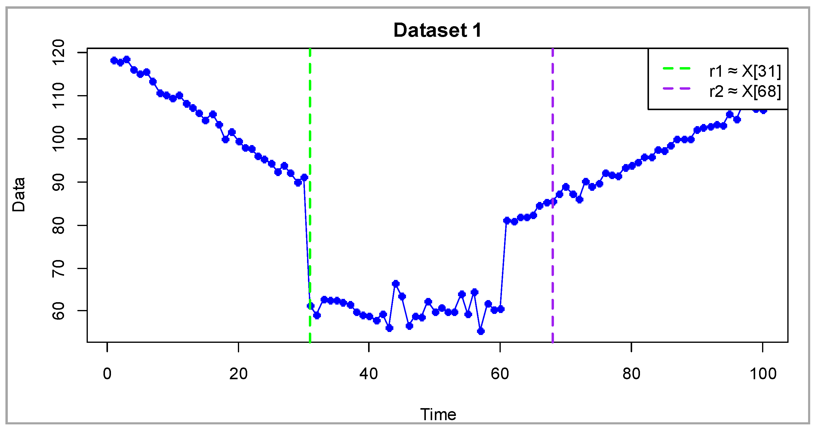
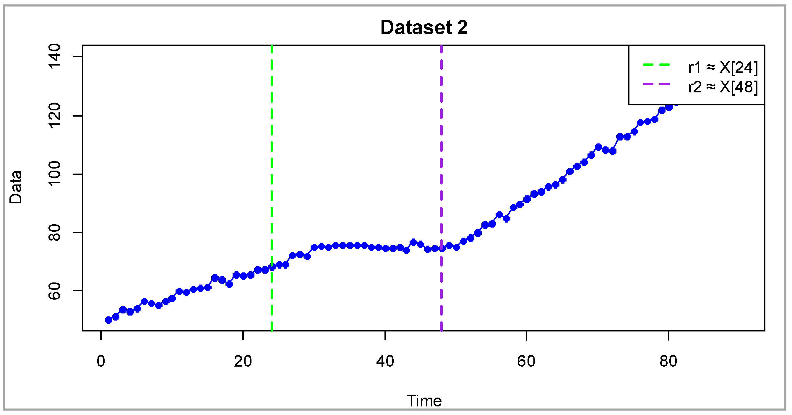
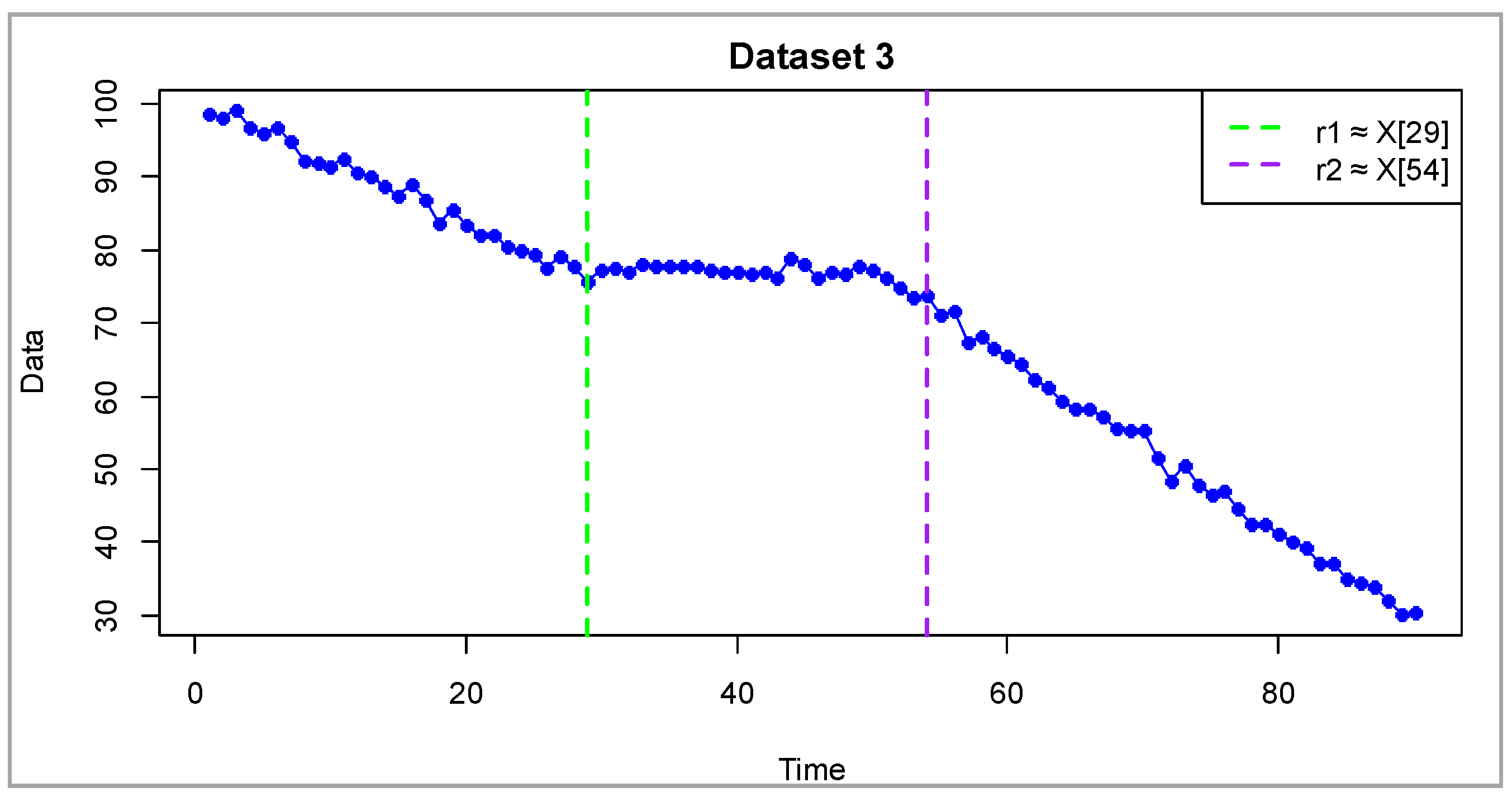
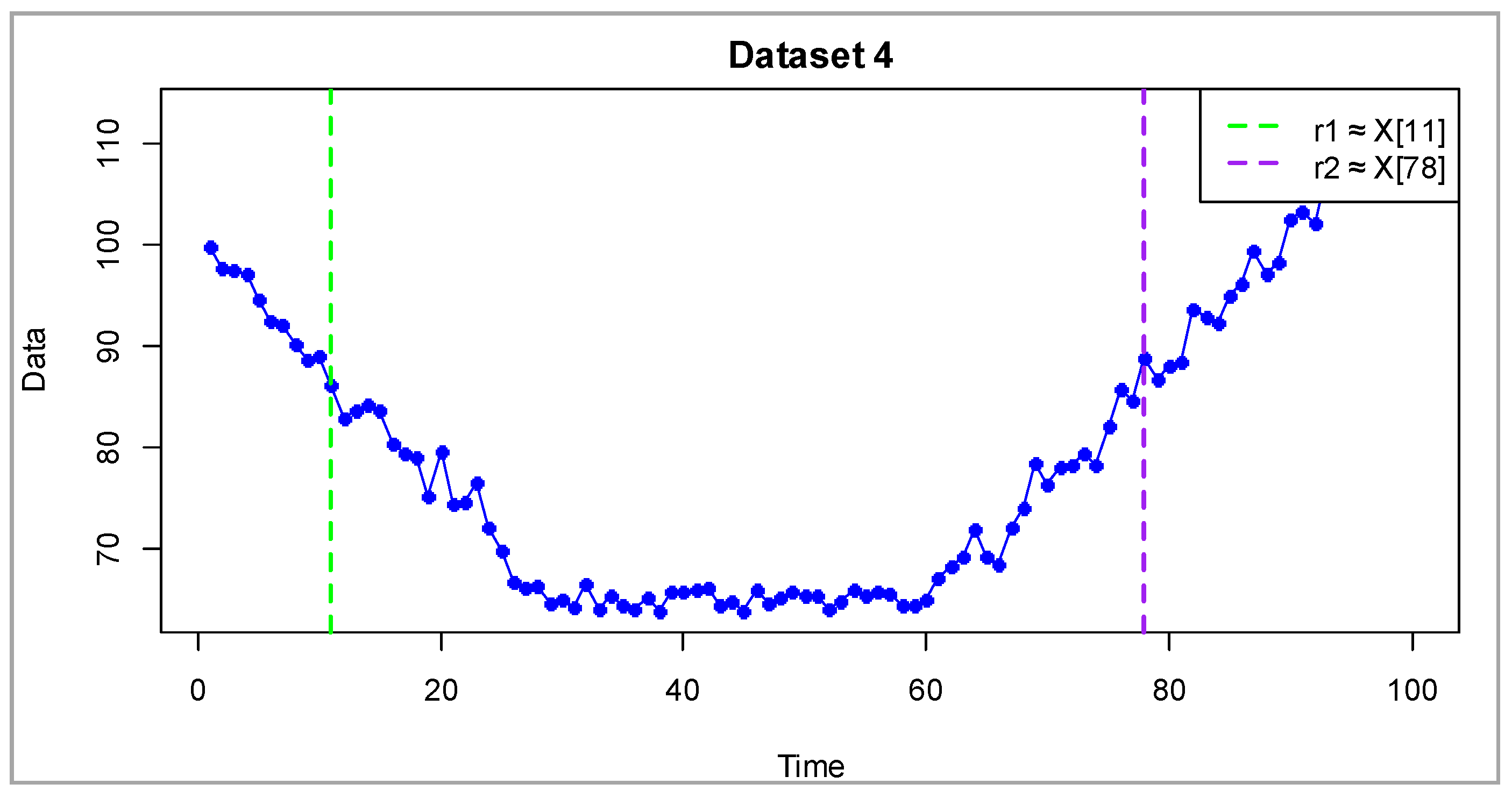
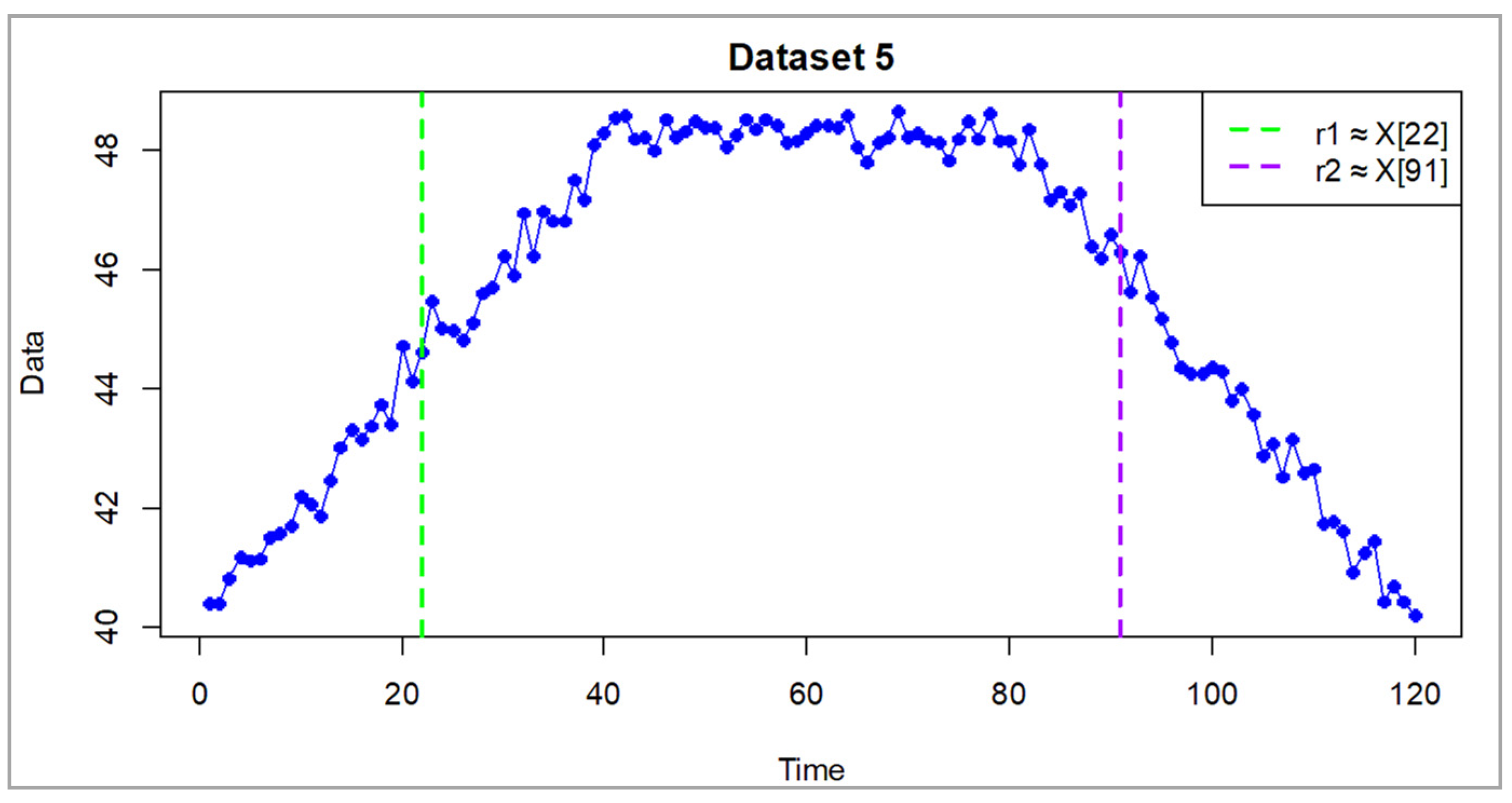
Figure 2, Figure 3, Figure 4, Figure 5 and Figure 6 display the time series trajectories , and displays the optimal value of the thresholds that record the transition between modes. The generated time series included a linear shift (characteristic for each data slice) and was supplemented with Gaussian noise with different variance. The entire dataset was combined into a set of values .

Figure 2.
Synthetic dataset 1 (dimensionless). Blue dots represent simulated observations. Vertical dashed lines show thresholds and , dividing the process into three regimes: (decreasing, ), (nearly stationary, ), and (increasing, ).
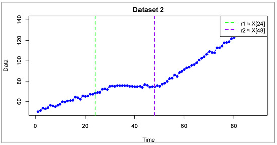
Figure 3.
Synthetic dataset 2 (dimensionless). Blue dots represent simulated observations. Vertical dashed lines show thresholds and , dividing the process into three regimes: (increasing, ), (nearly stationary, ), and (increasing, ).
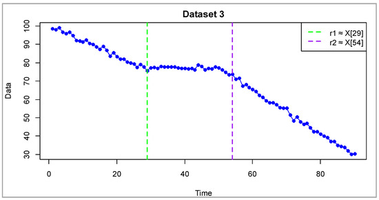
Figure 4.
Synthetic dataset 3 (dimensionless). Blue dots represent simulated observations. Vertical dashed lines show thresholds and , dividing the process into three regimes: (deceasing, ), (nearly stationary, ), and (decreasing, ).
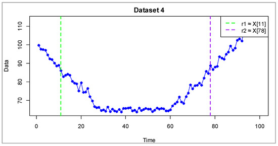
Figure 5.
Synthetic dataset 4 (dimensionless). Blue dots represent simulated observations. Vertical dashed lines show thresholds and , dividing the process into three regimes: (decreasing, ), (nearly stationary, ), and (increasing, ).
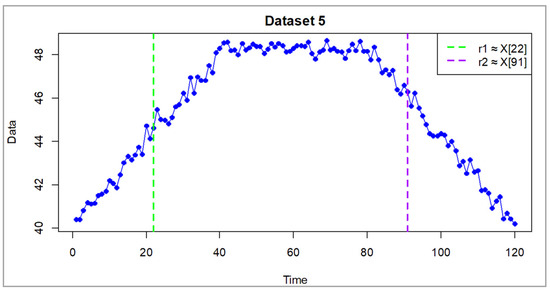
Figure 6.
Synthetic dataset 5 (dimensionless). Blue dots represent simulated observations. Vertical dashed lines show thresholds and , dividing the process into three regimes: (increasing, ), (nearly stationary, ), and (decreasing, ).
Comparison between approximate true (True, approx.) and estimated (Estimated) threshold values and for five synthetic datasets Table 1. The true thresholds were determined from the transition points between the three regimes () in the generated time data. In most cases, the estimated parameters are close to the original ones, confirming the stability of the estimation algorithm; minor discrepancies can be attributed to the stochastic nature of the process and the non-convex shape of the likelihood surface.

Table 1.
Approximate and estimated threshold.
The obtained results indicate that the algorithm reconstructs the threshold values with a small absolute error (within 0–6.8) and a relative error not exceeding 9%, confirming the high accuracy of parameter estimation across different datasets.
The graphs below, based on Dataset 4, illustrate the results from a different analytical perspective, providing a deeper view of the process dynamics and its structural features.
Figure 5 shows the time series of the observed process together with the estimated thresholds and . The green dashed line corresponds to the lower threshold , which is localized within the descending segment of the trajectory, while the purple line represents the upper threshold , associated with the phase where the process begins to rise. This threshold configuration intuitively aligns with the phase behavior of the series: the lower threshold separates the declining regime, whereas the upper one marks the recovery phase and the transition to growth.
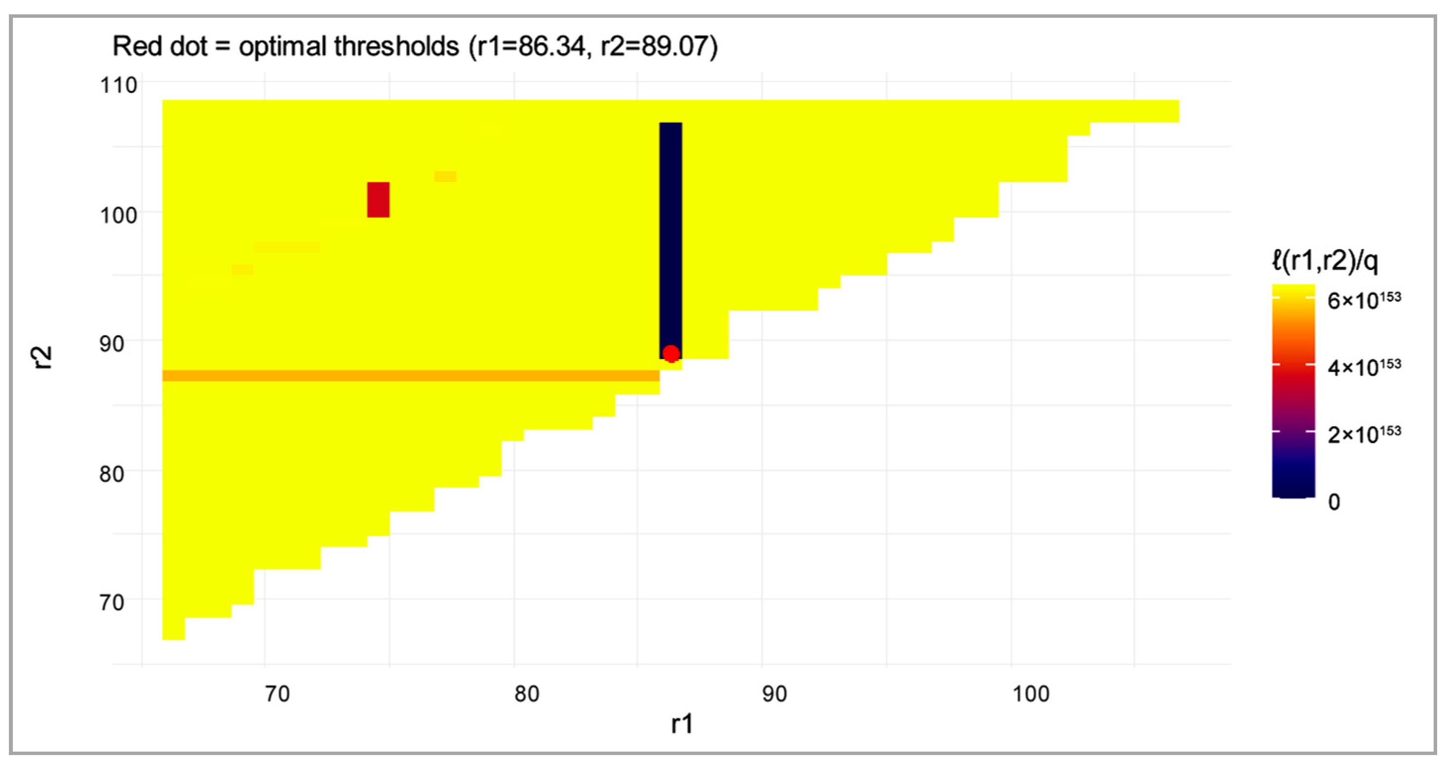
Figure 7 presents the likelihood function map in the space of the threshold parameters and . The color scale represents the normalized log-likelihood value averaged per observation: lighter areas correspond to higher (worse) criterion values, while darker regions indicate a better model fit to the data. The red dot marks the minimum corresponding to the estimated optimal thresholds. As seen from the figure, the surface exhibits a distinctly non-convex structure: most of the parameter space yields a poor fit, whereas the global minimum is concentrated within a narrow, localized region.

Figure 7.
Average log-likelihood per observation (normalized).
Thus, the combination of these two illustrations demonstrates, first, the interpretability of the estimated thresholds in the time-series dynamics and, second, confirms the validity of the chosen optimization procedure even under a non-convex likelihood surface. This highlights the effectiveness of the proposed approximate maximum likelihood method for estimating the parameters of the two-threshold model.
Figure 8 illustrates the three-dimensional landscape of the likelihood function in the parameter space of and . The red dot indicates the optimal threshold values and corresponding to the global minimum of the function. This representation clearly demonstrates the shape of the surface, the location of local and global minima, and allows for a visual assessment of the structure (non-convexity) of the optimization problem.
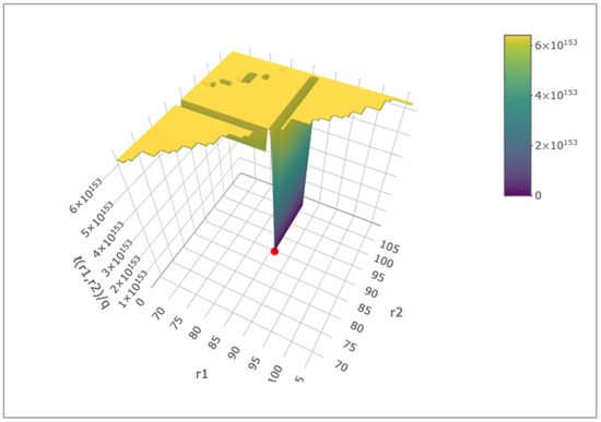
Figure 8.
Three-dimensional likelihood surface with optimal thresholds.
Figure 9 shows cross-sections of the likelihood surface for fixed values of . As varies, the function exhibits several local minima, confirming its non-convex nature. This explains why the estimation results may be sensitive to the initial parameter values and require careful selection of starting points or multiple runs of the algorithm with different initializations.
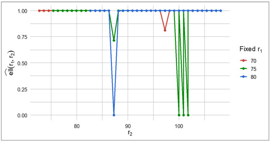
Figure 9.
Cross-sections of the likelihood surface at fixed values.
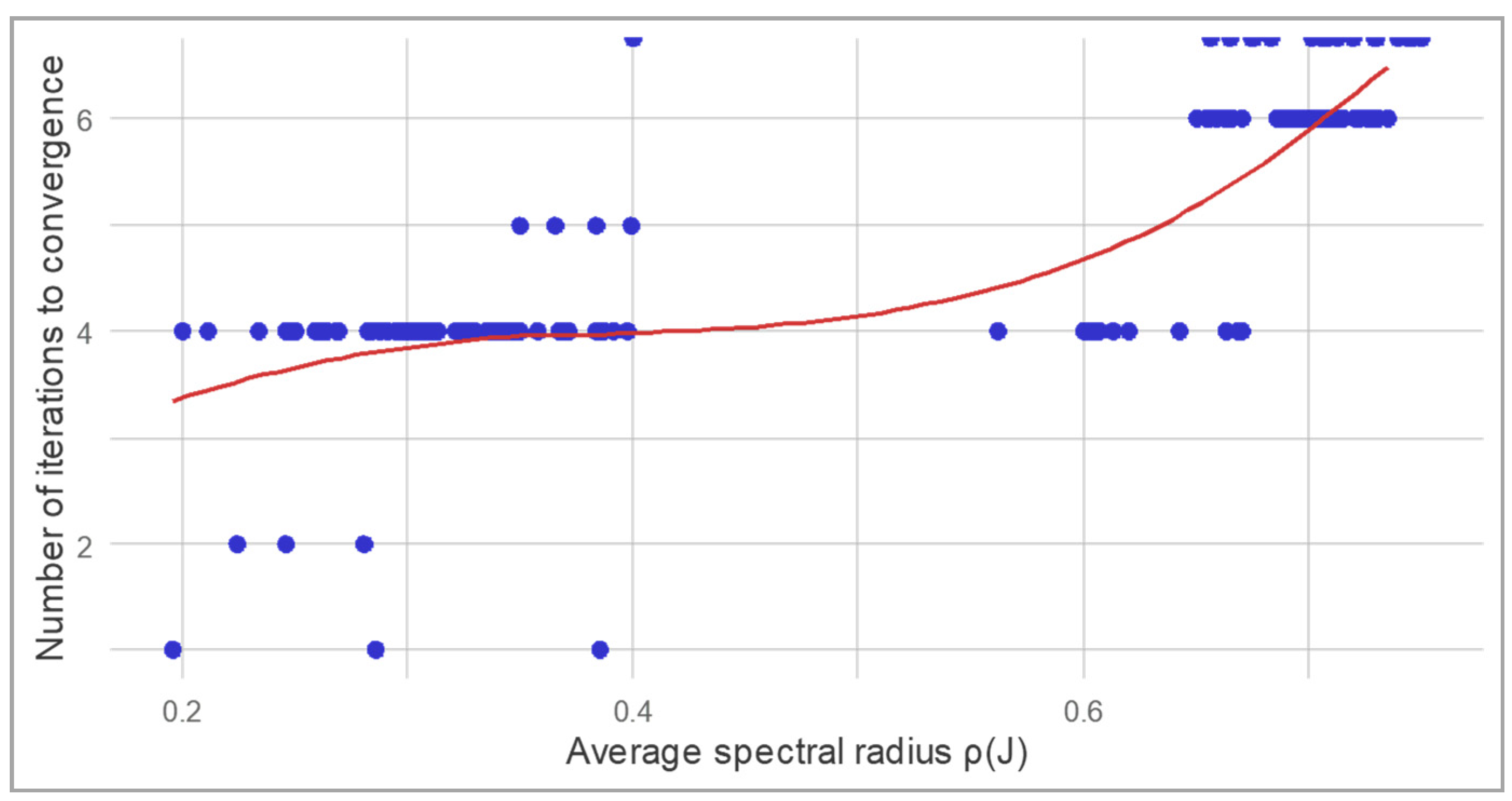
Figure 10 shows how the number of iterations required for convergence depends on the average spectral radius of the Jacobian matrix . Blue dots represent the results for different pairs of thresholds (), while the red curve shows a smoothed approximation illustrating the general trend of the relationship between the convergence rate and the spectral radius. It can be seen that for small values , the algorithm typically converges within 3–4 iterations, whereas as the spectral radius increases, the number of iterations rises significantly. This confirms the theoretical statement that the convergence rate of the iterative process is inversely related to the spectral radius of the Jacobian matrix.

Figure 10.
Dependence of the convergence rate on the spectral radius.
Using dataset 4 as an example, we assess several quantitative indicators of the model’s accuracy in reproducing the process dynamics, namely the Root Mean Squared Error (RMSE), Mean Absolute Error (MAE), and Normalized Root Mean Squared Error (NRMSE).
According to the simulation results for dataset 4, the root mean squared error of increments was RMSE = 2.04, and the mean absolute error was MAE = 1.56, which is comparable to the standard deviation of noise . Thus, the method adequately reproduces the stochastic component of the data.
The normalized error (NRMSE ≈ 0.97) indicates a close correspondence between the model and the empirical increments. The lowest accuracy is observed in the middle (second) regime, where the number of observations is minimal (n2 = 6).
The algorithm achieved convergence after 8 iterations for the set of parameters corresponding to the minimum value of the likelihood function. The computation time directly depends on the processing power of the personal computer on which the program code is executed.
These visualizations confirm the model’s ability to accurately detect regime changes, particularly when the signal-to-noise ratio is favorable. Higher dispersion may obscure threshold detection, but when transitions are distinct and noise is moderate, the algorithm reliably identifies structural shifts. Even under smooth trends and low noise, the method successfully captures changes in the data’s dynamic structure, demonstrating flexibility and robustness across a range of scenarios.
6. Conclusions
This study demonstrated the effectiveness of using approximate maximum likelihood to calculate the parameters of a two-mode pre-threshold process. The developed methodology made it possible not only to calculate the shift and dispersion parameters for the Ornstein–Uhlenbeck process modes, but also to determine the threshold points and , which divided the process dynamics into different segments with different properties. The implementation of the iterative algorithm in the program code confirmed the correctness of the calculations, and also revealed sensitivity to changes in the process data structure.
Compared to the methods proposed in [8], where a single-threshold model is considered, the pre-threshold model considered above allowed us to describe more complex, three-phase process dynamics. The study [9], which is based on the approximation of Lévy processes, illustrated the potential of using a two-threshold model in more complex stochastic processes.
As a result of this study, a logarithmic likelihood function with two thresholds was developed, the shift and dispersion parameters were estimated in the modes , , , an iterative algorithm for parameter estimation was implemented and its software implementation was developed.
Overall, the results confirmed that the proposed AMLE-based algorithm provided stable and accurate parameter recovery across different scenarios and noise levels. The findings provide a foundation for applying the two-threshold model to real-world time series data. This is particularly relevant in finance and related disciplines. The results also open opportunities for extending the approach to multidimensional threshold models based on the Ornstein–Uhlenbeck process.
Author Contributions
Conceptualization, S.B., A.N. and S.N.; methodology, A.N., S.B. and S.N.; formal analysis, S.B. and A.N.; investigation, A.N., S.B. and S.N.; writing—original draft preparation, A.N., S.B. and S.N.; writing—review and editing, A.N., S.B. and S.N.; project administration, S.B.; funding acquisition, S.B. All authors have read and agreed to the published version of the manuscript.
Funding
This research was funded by Ministry of National Defence of Lithuania, Study Support Projects NoV-58, 30 January 2025, General Jonas ŽemaitisMilitary Academy of Lithuania, Vilnius, Lithuania.
Data Availability Statement
The complete dataset supporting the reported results is available at: https://zenodo.org/records/16282478.
Conflicts of Interest
The authors declare no conflicts of interest.
References
- Chiou, Y.Y.; Su, L.; Tsai, H. Nonparametric Regression with Multiple Thresholds: Estimation and Inference. J. Econom. 2018, 206, 472–514. [Google Scholar] [CrossRef]
- Scarffe, A.; Coates, A.; Brand, K.; Bikker, M.; Cowan, K. Decision Threshold Models in Medical Decision Making: A Scoping Literature Review. BMC Med. Inform. Decis. Mak. 2024, 24, 273. [Google Scholar] [CrossRef] [PubMed]
- Lejay, A.; Pigato, P. A Threshold Model for Local Volatility: Evidence of Leverage and Mean Reversion Effects on Historical Data. arXiv 2017, arXiv:1712.08329. [Google Scholar]
- Rowland, M.; Tozer, T.N. Clinical Pharmacokinetics and Pharmacodynamics: Concepts and Applications; Lippincott Williams & Wilkins: Philadelphia, PA, USA, 2011. [Google Scholar]
- Gonzalo, J.; Pitarakis, J.-Y. Estimation and Model Selection Based Inference in Single and Multiple Threshold Models. Rev. Econ. Stud. 2002, 69, 813–833. [Google Scholar] [CrossRef]
- Tong, H.; Lim, K.S. Threshold Autoregression, Limit Cycles and Cyclical Data. J. R. Stat. Soc. Ser. B Methodol. 1980, 42, 245–292. [Google Scholar] [CrossRef]
- Uhlenbeck, G.E.; Ornstein, L.S. On the Theory of Brownian Motion. Phys. Rev. 1930, 36, 823–841. [Google Scholar] [CrossRef]
- Yu, T.-H.; Tsai, H.; Rachinger, H. Approximate Maximum Likelihood Estimation of a Threshold Diffusion Process. Comput. Stat. Data Anal. 2020, 142, 106825. [Google Scholar] [CrossRef]
- Tsai, H.; Nikitin, A.V. Threshold Models and Approximate Maximum Likelihood Estimation of Lévy Processes. Cybern. Syst. Anal. 2024, 60, 123–140. [Google Scholar] [CrossRef]
- Milstein, G.N. Numerical Integration of Stochastic Differential Equations; Kluwer Academic Publishers: Boston, MA, USA, 1995. [Google Scholar]
- Ji, L.; Li, C.; Zhou, X. Threshold Diffusions. arXiv 2025, arXiv:2508.17812. [Google Scholar] [CrossRef]
- Rachinger, H.; Lin, E.M.H.; Tsai, H. A Bootstrap Test for Threshold Effects in a Diffusion Process. Comput. Stat. 2023, 38, 901–919. [Google Scholar] [CrossRef]
- Aït-Sahalia, Y. Maximum Likelihood Estimation of Discretely Sampled Diffusions: A Closed-Form Approximation Approach. Econometrica 2002, 70, 223–262. [Google Scholar] [CrossRef]
- Chan, K.S. Consistency and Limiting Distribution of the Least Squares Estimator of a Threshold Autoregressive Model. Ann. Stat. 1993, 21, 520–533. [Google Scholar] [CrossRef]
- Su, F.; Chan, K.S. Quasi-Likelihood Estimation of a Threshold Diffusion Process. J. Econom. 2015, 189, 473–484. [Google Scholar] [CrossRef]
- Li, C. Maximum-Likelihood Estimation for Diffusion Processes via Closed-Form Density Expansions. Ann. Stat. 2013, 41, 1350–1380. [Google Scholar] [CrossRef]
- Mazzonetto, S.; Pigato, P. Drift Estimation of the Threshold Ornstein–Uhlenbeck Process from Continuous and Discrete Observations. arXiv 2022, arXiv:2008.12653v3. [Google Scholar] [CrossRef]
- Tong, H. Non-Linear Time Series: A Dynamical System Approach; Oxford University Press: Oxford, UK, 1990. [Google Scholar]
- Gelman, A.; Carlin, J.B.; Stern, H.S.; Dunson, D.B.; Vehtari, A.; Rubin, D.B. Bayesian Data Analysis, 3rd ed.; CRC Press: Boca Raton, FL, USA, 2013. [Google Scholar]
- Dempster, A.P.; Laird, N.M.; Rubin, D.B. Maximum Likelihood from Incomplete Data via the EM Algorithm. J. R. Stat. Soc. 1977, 39, 1–22. [Google Scholar] [CrossRef]
- Skorohod, A.V. Studies in the Theory of Random Processes; Reprinted Edition; Dover Publications: New York, NY, USA, 1962. [Google Scholar]
- Livina, V.N.; Lenton, T.M. A Modified Method for Detecting Incipient Bifurcations in a Dynamical System. Geophys. Res. Lett. 2007, 34, L03712. [Google Scholar] [CrossRef]
- Kelley, C.T. Iterative Methods for Linear and Nonlinear Equations; Society for Industrial and Applied Mathematics: Philadelphia, PA, USA, 1995; p. 7. [Google Scholar]
- Burden, R.L.; Faires, J.D. Numerical Analysis, 9th ed.; Cengage Learning: Boston, MA, USA, 2011; pp. 60–62. [Google Scholar]
- Kloeden, P.E.; Platen, E. Numerical Solution of Stochastic Differential Equations; Springer: Berlin/Heidelberg, Germany, 1992; pp. 287–289. [Google Scholar]
- Higham, D.J. An Algorithmic Introduction to Numerical Simulation of Stochastic Differential Equations. SIAM Rev. 2001, 43, 525–546. [Google Scholar] [CrossRef]
Disclaimer/Publisher’s Note: The statements, opinions and data contained in all publications are solely those of the individual author(s) and contributor(s) and not of MDPI and/or the editor(s). MDPI and/or the editor(s) disclaim responsibility for any injury to people or property resulting from any ideas, methods, instructions or products referred to in the content. |
© 2025 by the authors. Licensee MDPI, Basel, Switzerland. This article is an open access article distributed under the terms and conditions of the Creative Commons Attribution (CC BY) license (https://creativecommons.org/licenses/by/4.0/).

